Household-differentiated demand modelling for communities

HOUSEHOLD-DIFFERENTIATED DEMAND MODELLING FOR COMMUNITIES

Graeme Flett and Nicolas Kelly

Energy Systems Research Unit, University of Strathclyde, Glasgow, UK

ABSTRACT

Micro-generation schemes are increasingly being proposed for and incorporated in new-build housing developments. Community composition dependant demand prediction for such schemes is poorly understood and modelled.

Using a previously developed higher-order Markov-chain occupancy model, differentiated for different household types, an occupancy-driven electricity demand model has been developed from high resolution appliance-level data to realistically distribute demand cycles for individual households. The model incorporates a novel event-based method for linking the time-of-day probability of appliance cycles relative to occupancy, which allows accurate replication of expected demand patterns and improves computational efficiency compared to existing models. Additional socio-economic and behavioural factors are also included to better capture demand diversity.

INTRODUCTION

The ability to predict time-dependant energy demand is important for all scales of energy system development. For the national grid, detailed demand prediction allows the need for supplementary generation to be scheduled. At this scale, however, the influence of individual households or groups of distinct household types is negligible. However, when considering community-scale energy systems such as micro grids, the numbers of end users is far smaller (typically <<1000), with a corresponding increase in the influence of different household behaviours.

Limited research has been done on the relationship between the size and composition of a community, and its demand characteristics. Integration of renewable-based schemes, with intermittent or variable supply and the need for wider grid back-up, requires a greater understanding of demand patterns to ensure the optimum mix of supply, storage, and grid import and export is specified. The UK government has identified this lack of understanding of demand as a key barrier to growth in low-carbon

community energy and demand management projects (DECC, 2014).

Occupancy Influence on Demand

A significant number of factors have been shown to influence household energy demand characteristics. Yohanis (2008), and Haldi and Robinson (2011) have shown that these include, but are not limited to, house size, household size, bedroom number, occupant age, income, children, and tenure.

Yao and Steemers (2005), and Torriti (2012), amongst others, have shown that the distinct occupancy patterns associated with different types of households strongly influence demand characteristics. This is unsurprising as a large proportion of energy use requires an active occupant to initiate demand. Limited work exists that analyses occupancy data per occupant, household and day type (e.g. weekday, weekend) to allow the occupancy-driven contribution to household energy demand to be accurately modelled.

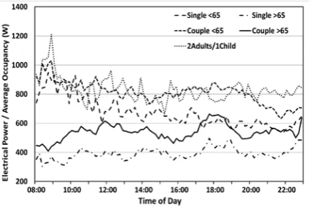
The UK 2010-2011 Household Electricity Survey (HES) measured electricity demand in 251 households at the appliance level (DECC, 2012). Initial reporting of the results has shown that there are distinct demand variations between identified household types such as single non-pensioner; single pensioner; pensioner couple; family and multi-adult households.

Figure 1 shows the average weekday electrical demand divided by the average occupancy probability for different smaller household types and age ranges. The relatively flat profiles demonstrate that there is a strong link between occupancy and demand at this level of household differentiation, but also that other factors need to be included that account for the residual variation.

REVIEW

Occupancy-driven Demand Models

Bottom-up energy models using occupancy as the foundation represent a key subset of existing models. A demand model review by Grandjean et al (2012) found those using Time-use Survey (TUS) based occupancy models to be most effective. Key existing models of this type are Richardson et al (2010), Widen and Wackelgard (2009), and Wilke (2013).

Each of these existing models has limitations: • The ‘Richardson’ model uses a first-order,

Markov-based occupancy model and differentiates households based only on occupant number, ignoring other characteristics. Appliance cycles are linked to broad TUS activities, without any diversity except for a general ownership probability.

• The ‘Widen’ model treats each occupant independently ignoring family inter-relationships. It incorporates a Markov-based occupancy model that differentiates ‘active’ occupancy into 7 major TUS-derived activities, increasing the data requirement. Appliance use is allocated probabilistically based on identified TUS activity. • The ‘Wilke’ model uses a different event-based occupancy-modelling approach. This was shown to be less accurate than an equivalent Markov approach (Flett and Kelly, 2014). The demand model uses time-dependent power functions linked to TUS activities to determine average profiles rather than a bottom-up approach and is less relevant for modelling demand variability.

Time-Use Survey Activities and Demand

The majority of existing bottom-up residential demand models use TUS activities to define when appliances are likely to be used.

TUS activities do not typically have a direct relationship with a specific appliance use. ‘Food Prep’, ‘Laundry’ and ‘Wash and Dress’, for example, are broad TUS activity definitions that do not necessarily relate to energy use. Integrating TUS activities within an energy model therefore requires that the relationship between activity and appliance use is defined.

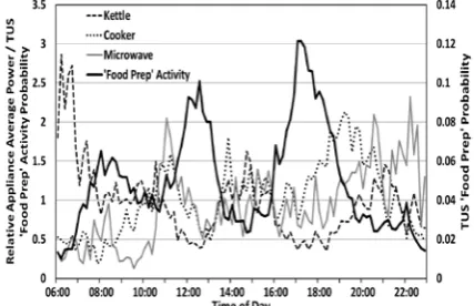
Figure 2 shows the relative average power per main cooking appliance divided by the proportion of

households with the ‘Food Prep’ TUS activity from the UK 2000 TUS survey (ONS, 2003). Only 1-person households were analysed to remove any multiple occupancy influences. The results clearly show little correlation between the TUS activity and energy use, suggesting that for individual cooking appliances, ‘Food Prep’ is a poor usage predictor. There is also some evidence that for short cycle appliances (e.g. kettle), the 10-minute resolution TUS activity basis may not reliably capture use (e.g. the peak average kettle power for all households with the ‘Food Prep’ activity exceeds a typical unit power suggesting some kettle use during periods with other stated activities.)

Figure 2: Average relative cooking appliance power normalised for TUS ‘Food Prep’ activity probability

Similar results can be shown for the majority of other relevant TUS activity-appliance combinations. The exception being TV use.

A further concern with current models utilising TUS activities is that all are first-order (i.e. only current activity is considered for activity transition prediction and not an extended sequence). Potentially resulting in unrealistic repetitions of common activities.

The availability of detailed appliance level data from the Household Electricity Survey (HES) gives a means of identifying appliance cycle frequencies and time of day usage probability without the need for TUS activities as an intermediate step. HES data is also available over a minimum of one month. This allows better assessment of the demand variation over time as TUS diaries are limited to only 24 hours. The main limitation of the HES dataset is that occupancy data is not included.

Previously Developed Occupancy Model

Interactions between related adults (e.g. a co-habiting couple) have been captured by treating each pair as a single entity. Child occupancy is directly linked to parent occupancy using a simplified Markov model. Other occupant types (e.g. single householders, adult children and households comprising unrelated adults etc.) are modelled as individuals. Each distinct overall household occupancy profile is generated from the required combination of couple, individual adult and child models. Day types for each are split into working and non-working days, for weekdays, Saturdays and Sundays.

The model also uses a higher-order Markov technique that takes the duration of an activity into account when predicting future activity. This is shown to improve on existing first-order and non-Markov higher-order models with regards to occupancy prediction. Annual occupancy profiles for each household are produced based on assigned calendars of day types based on a realistic distribution of employment type, typical work weeks, and school term times.

The occupancy model is used as the foundation for the demand model presented in this paper.

AIM

The overarching aim of the presented work is to allow prediction of the potential variations in demand for community-scale energy schemes as a result of different community compositions and the natural variability within communities with the same basic characteristics. Using the previously developed differentiated occupancy model (Flett and Kelly, 2014) to capture occupancy patterns associated with each household type, improvements to appliance cycle prediction and demand diversity modelling were sought.

A secondary aim was to generate a demand model that could provide realistic annual energy use distributions capturing overall, seasonal and inter-day diversity of use. Applied to communities this would allow energy-use diversity to be assessed both at high time resolution and over extended timescales.

MODEL DEVELOPMENT

The following section describes the electrical demand model development.

Electrical Dataset

Fundamental to the development of the demand model was access to detailed appliance-level data for a significant number of households. The developed model is based on electrical data provided by the Household Electrical Survey (HES) (DECC, 2012). Individual appliances in 251 UK households were monitored for 1-2 months with a 2-minute resolution,

with 26 households also monitored for a full year at a 10-minute resolution.

It is assumed that this data is broadly representative of appliance use for the UK. As the dataset only includes private households it is likely that it represents an above average socio-economic group. The use of independent appliance ownership data for major appliances and normalising the model based on an income factor (described below) should, to some degree, mitigate this shortcoming in the dataset.

Electrical Appliance Data Analysis

The detail provided by the HES dataset allows both high-level analysis to determine the distribution of cycles between households, and detailed analysis of the timing of cycles. As stated, a limitation of the dataset is there is no corresponding occupancy data. For occupancy-related analysis, the TUS-identified average occupancy for the equivalent household type has been used.

Where data has been differentiated by household type, the following groups have been used; single, single pensioner, pensioner couple, family and multi-adult. If sufficient data is available (i.e. for commonly owned appliances (e.g. cooker, kettle)) occupant number has also been used for family and multi-adult households.

Each appliance has been analysed for the following: • Average Cycles per Household Type (AC_HT):

Average cycles per day, or daily usage probability and average number of cycles per day used, for each appliance (depending on whether appliance is modelled as ‘simple’ or ‘complex’ as defined below) for each household type has been determined. For kettle, microwave, and tumble dryer use, clear seasonal demand variations have also been captured using a sinusoidal function.

• Average Cycle Distribution (ACD): To capture the variable demand within each household type, the distribution of cycle number/probability to the household type average is determined. The distribution of the actual/average ratios is used as a proxy for the behavioural distribution for all households. For each modelled household the factor is allocated randomly from this overall distribution.

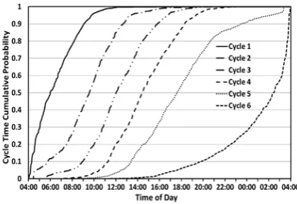
• Cycle Time: Separate cycle start time distributions are captured split by total number of daily cycles and specific cycle number (see Figure 3). These are used as the basis for linking occupancy with appliance use potential as described in detail below.

To account for different base and variable cycle power, a nominal duration is determined by dividing total cycle power by a fixed average cycle power.

Additional Demand Factors

Household demand is a complex interaction of different factors. In addition to the household type-based average use and appliance-level behavioural variation, the following are also used in the model; (1) basic appliance ownership, (2) relative occupancy, (3) income, and (4) overall energy behaviour.

• Ownership: Major appliance (washing machine, dryer, dishwasher, microwave, PC) ownership probability is taken from the 2011 UK ONS Family Spending survey (ONS, 2012) based on household type and income decile. Ownership of other appliances is from the HES dataset distribution.

• Occupancy Factor (AOF): Without integrated occupancy and appliance usage data an explicit assessment of the impact of occupancy duration on the daily and overall number of appliance cycles is difficult. Factors have been set using common sense assessments but would benefit from observational validation. For example, in Equation (1), for a kettle an occupancy factor of 0.5 is used and for washing machines a lower value of 0.1 is used. The factor is also used to assess occupancy influence on the daily use potential for each household.

• Income Factor (IF): The influence of income on appliance and energy use is complex. Ofgem (2010) shows that low income households can have high consumption and vice versa, although there is a broad correlation between income and demand.

Data from Ofgem (2010) is used to determine the relative energy use per consumption decile, and the probability of a particular household residing in an energy consumption decile based on income decile. Each household modelled is probabilistically allocated an income decile (based on national survey data), and from this a consumption decile and a relative energy consumption factor from the Ofgem-derived data are determined.

Jamasb & Meier (2010) have calculated the income-specific elasticity in energy demand to be 0.06 (log of expenditure per log of income). Analysis of the Ofgem data gives an equivalent elasticity of 0.18 if all influences, not solely income, are included. Therefore the income-specific relative consumption factor is assigned with an exponent of 0.33 (0.06/0.18).

• Overall Behaviour Factor (OBF): Analysis of the HES data corroborates that of Gill et al (2010) that there is little evidence of a strong link between relative individual appliance use and overall demand. The exception is a small percentage of very low and high consumers who have consistent extreme use.

Gill et al determined that 37% of electricity use can be attributed to behaviour independent of identifiable household characteristics. An additional overall factor is therefore applied selected randomly between 0.77 and 1.23 (equivalent to a 37% variation). Assuming a linear distribution is likely to be an over-simplification, but further work is required to determine if there is a more complex link between this factor and other household characteristics.

Overall Cycle Number/Probability Determination

For each household and per owned appliance, the average number of cycles per day (simple appliances) or daily use probability (complex appliances) is therefore calculated from the following equation:

𝐴𝐴𝐴.𝐶𝐶𝐶. =𝐴𝐶_𝐻𝐻×𝐴𝐶𝐴×𝑅𝑅𝑅𝑅𝐶𝐶𝐴𝐴𝐴_×𝐼𝐼0.33

×𝑅𝑂𝐼 (1)

Electrical Cycle Model Types

Five different appliance cycle models have been developed; fixed, simple, complex, lighting and TV. As defined below, each differs in the dataset analysis used, extent of occupant influence, and dependence on recent use.

Fixed Cycle

Fixed cycle appliances have an energy demand that is largely independent of occupancy. This primarily applies to cold appliances.

Baseline power ratings for each cold appliance assigned is based on the HES dataset distribution of energy ratings and volumes. A sinusoidal time of day and day of year variation is applied based on dataset analysis to account for typical variations in door opening probability and household temperature.

Simple Cycle

For certain appliances the daily demand probability is assumed to be based on short-term need and independent of use on preceding days. This applies, for example, to smaller kitchen appliances (kettle, microwave etc.), and IT equipment.

distribution produced a more accurate distribution than either Poisson or Normal equivalents).

Complex Cycle

Other appliances, such as washing machines and dishwashers, have usage patterns that extend over a number of days driven by a need that increases with time. Demand likelihood is linked both to the daily use probability and the time since last use. Previous modelling techniques have not attempted to model this dependence, which potentially results in unrealistic cycle patterns.

Daily use probability is assigned for each household in the same manner as the daily cycle number for ‘simple’ appliances. The number of cycles per use day is assigned using a separate probability model.

Analysis of the gaps between days of use (i.e. ‘next-day’, ‘next-day+1’ etc.) for all relevant appliances showed that the distribution was highly random but constrained by an upper limit of approximately twice the average (i.e. if used every 3 days on average, the maximum ‘gap’ is c. 6 days). A ‘gap’ probability model was developed based on this apparent randomness within defined limits.

The model assigns an upper gap limit of twice the average ‘gap’ value +/- 0.5 days. The minimum and maximum ‘next-day’ use probability that would allow both the daily use probability and upper limits to be achieved is then calculated. A ‘next-day’ use probability is selected randomly between the min and max values and the residual probability determined. This process is then repeated for subsequent numbers of gap days (‘next-day+1’ etc.) until the cumulative probability reaches 1.

The appliance cycle model uses the cycle gap probability distribution to determine the number of days to the next cycle from the preceding cycle.

Lighting

The HES dataset has lighting power data at the main distribution boards (typically by floor) and for individual lamps. Also included is average installed lighting power per room and percentages of low energy bulbs per-house. However, there is no room level per-timestep data.

As a result, a lighting model based first on inferred occupant location from modelled appliance/hot water use and then TUS activity probability to fill gaps was used. This is primarily a means to model location sharing and transition likelihood, and therefore realistic lighting levels and level changes. The concept is similar to that used by Terry et al (2013). The HES data was used for lighting power per room and low-energy bulb proportion, and for validation.

The range of threshold solar levels for switching events was determined by comparing timings from the HES data with average UK-wide solar levels. The

model specifically uses 1-minute resolution solar data from Glasgow to determine lighting demand.

Terry et al (2013) highlighted levels of day and night use in the HES data that could not be directly attributed to external solar levels or occupancy respectively. Lighting use for the 11am-1pm and 2am-4am periods was analysed to determine probability of use and power used relative to a mid-evening base level. Each modelled household was randomly assigned a day and night use probability from the distribution.

TV

A secondary Markov model is applied to each active occupancy period to determine if the occupant is either generally active or watching TV based on TUS activity reporting.

Appliance Cycle Start Model

For each HES-monitored appliance modelled with the ‘simple’ or ‘complex’ cycle model, the range of cycle start times was analysed based on number of cycles per day and for each cycle number.

The influence of the specific number of occupants on appliance use was also analysed by comparing average power with average total occupancy from TUS data. Only for cooker, microwave and dishwasher use was the influence of occupant number identifiable.

The overall cycle start distribution was then factored by the relevant occupancy probability (overall or occupant number as above) for each household type to eliminate occupancy influence. These final distributions reflect cycle start time probability if a particular household type is occupied.

An example set of occupancy-normalised cycle time curves for a kettle 6-cycle day are shown in Figure 3.

Figure 3: Cumulative probability distribution of kettle cycle times for a 6 cycle day

occupancy and appliance availability to be greater than zero.

Table 1

Occupancy/Appliance Event Matrix Example

Timestep 230 305 413 556 910 989 1195 Occupants 1 0 1 0 1 2 0 Avail. 1 1 1 1 1 1 1 Clt.Prob. 0.21 0.41 0.61 0.67 0.85 0.91 0.98

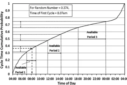
The appliance-use cumulative probability (Clt.Prob.) at the start and end of each ‘available’ period are determined and a random number generated (limited to values within the ‘available’ periods) to determine the cycle time (see Figure 4). Cycle times therefore have a higher probability during periods with higher typical occupancy-normalised use.

Figure 4: Cycle time prediction model example

For subsequent cycles, the previously identified cycle period (including a ‘dead’ period pre- and post-cycle) is added as an unavailable period (see Table 2). The next cycle time is determined in the same manner using the relevant start time probability distribution.

Table 2

Cycle/Unavailable Period Added to Event Matrix

Timestep 230 290 303 305 413 556 910 Occupants 1 1 1 0 1 0 1 Appl. Avail. 1 0 1 1 1 1 1

An additional benefit of this approach is that it does not require a computation per timestep for each appliance as with existing models which significantly reduces the computation time and allows annual 1-min resolution models to be feasible.

Linked Appliance Use

The TV model directly links TV use with other related appliances (DVD, Set Top Box etc.), and, similarly, the computer model links monitor, printer and router use with computer use (and for the router with basic occupancy). Parallel use probability was determined from HES dataset analysis.

Analysis of washing machine and tumble dryer use shows that there is a 64% probability of tumble dryer cycles following washing machine cycles on the same day (and 30% within 2 hours). Modelled

tumble dryer cycles are therefore linked to washing machine cycles based on the probability distribution.

Similar analysis of dishwasher use in relation to cooking activities, and of overlapping use of different cooking appliances showed some correlation but not distinct enough to justify modelling directly.

Shared Appliance Use

No dataset is available that analyses the extent of appliance sharing. For lighting and TV use, sharing is significant. Particularly as they are modelled from individual- rather than household-driven demand, with typically multiple available ‘units’.

The lighting model tracks location and where multiple people are in the same room the probability of additional lighting power being used increases.

TV power data was compared with average occupancy to determine the relative probability of shared use based on time of day. The baseline value is unknown and was set at 40% to fix the model average power as per the input data. Further work to determine this factor independently would be useful to allow this artificial calibration to be eliminated.

VALIDATION & RESULTS

As a first step, the model has been compared to the input data in order to determine the quality of calibration. Future, more rigorous validation will require comparison with an independent dataset.

Quality of Calibration

The current electrical model includes all major non-heating appliances (cold, cooker, kettle, microwave, toaster, washing machines, tumble dryers, dishwashers, audio-visual, IT, lighting). A small number of minor appliances, such as alarms, cordless phones, dehumidifiers etc., also need to be included, but these represent less than 10% of overall demand.

The baseline calibration data from the HES dataset has been compiled to reflect only the appliances currently modelled. A model has been set up that matches the characteristics and available appliance data for each household in the HES dataset. The restricted number of ‘appliances’ and lack of data for a small number of owned appliances means that this model does not reflect total demand but is a means to test the methodology using a representative subset.

The HES dataset includes basic socio-economic data. If required data is unavailable, it has been assigned based on national survey-based probabilities.

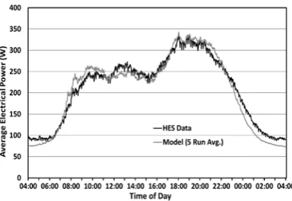
Figure 5: Per-Timestep Average Power Comparison for Full HES-replicating Population

Figure 5 shows the overall per-timestep average for all 251 modelled households. There is broad agreement between the data and model with, in particular, the timing of significant demand changes showing good agreement. (A planned improvement in the modelling of night-time active occupancy, which is currently underestimated, should improve the prediction during this period.)

Household Type Analysis

The results have been analysed for the household types used by HES; single non-pensioner; single pensioner; pensioner couple; family; multi-adult.

For all except the single non-pensioner (SNP) group there is close alignment between input data and model as demonstrated by the distinct pensioner couple profiles compared in Figure 6. The month-duration SNP group HES data is significantly skewed towards summer periods, and the data and model match closely when the model is restricted to the input data periods only. For the other populations, the input data has a representative distribution over all periods.

Figure 6: Per-Timestep Average Power Comparison for Pensioner Couple Households

Diversity Modelling

A key aim of the model is to capture demand diversity using the various factors identified above.

For community analysis this allows the potential variation in demand to be predicted accurately.

Results analysis (see Figure 7) shows that without the additional occupancy, income and overall factors the average power distribution remains broadly representative of the HES dataset distribution. This highlights that at this level of detail appliance ownership, random appliance-level cycle variation, occupant number, and household type are key drivers in overall demand diversity. However, the unfactored distribution is flatter than the measured distribution.

Including additional behavioural factors as defined above improves the ability of the model to replicate the low and high end power levels, but there remains some discrepancy. Further analysis at the household level will be required to determine if the individual factors and how they are combined is realistic.

Figure 7: Distribution of Average Power for HES Dataset and Full HES-replicating Population

FURTHER WORK

Figure 7 demonstrates that the model produces a realistic range of average electrical power demand levels per household and Figures 5 and 6 show that the overall and distinct household type overall demand profiles from the input data are replicated.

The current verification work has focused on household type groups and overall averages. Further work is required to confirm that individual household results are also representative of those in the input dataset and also of those from independent datasets. This will indicate to what level of detail the model is useful, whether for high-level, long-term average behaviour as already demonstrated or also for more specific factors, such as load peaks and diversity.

The model then needs to be validated against real community data to confirm the current assumption that the HES data is broadly representative.

the extent to which they and random behaviours may vary within a particular community.

DISCUSSION

No demand model can wholly predict realistic energy use at the household- or community-level given the range of influencing factors. The aim should be to provide microgeneration developers potential demand ranges with probabilities to allow sensible design decisions to be made with regard to generation, storage and distribution sizes.

The proposed model builds on a developed occupancy model that has significant differentiation based on household size and type. The demand model links to this model and has a similar degree of differentiation for energy use behaviours. New methods have been proposed for modelling individual appliances from high resolution, extended period demand data, linked to household occupancy. This allows appliance use to be realistically distributed at the intra-day level, over multiple days, and factored for seasonal influences. The model proposed in this paper has a range of probabilistic population composition, cycle and behaviour factors, therefore a number of runs is required to capture a representative range of potential households, to set a population baseline demand, and predict the potential variation from the baseline.

CONCLUSION

Existing bottom-up energy models have been limited by several factors which the work presented in this paper has attempted to address. These limitations are an inability to differentiate between different household types, limited intelligence in the allocation of appliance cycles based on time-of-day occupancy and use potential, and a lack of additional factoring to capture socio-economic and behavioural diversity.

The use of a household differentiated occupancy and appliance use model that accounts for specific patterns of use allows the influence of different household groups on demand to be assessed.

Appliance cycle starts are predicted based on occupancy and relative time-of-day use potential. This improves on models based on broad TUS activities which poorly predict specific appliance use.

Finally additional factors for relative occupancy, income and random behaviour influence are included to better capture realistic diversity of overall demand, although further calibration of these is required.

Limited input data and necessary averaging within household types means that this model is primarily relevant for groups of households and to assess relative differences based on group size and composition. Further analysis of household-level results will determine if the results can also be applied usefully to individual households.

ACKNOWLEDGEMENTS

We gratefully acknowledge the financial support received for this work from the BRE Trust and the access to the HES dataset granted by DECC.

REFERENCES

DECC. 2012. Household Electricity Survey. Electrical Appliance Use Dataset.

DECC. 2014. Community Energy Strategy: Full Report. A report by the Department for Energy and Climate Change. January 2014.

Flett, G., & Kelly, N. 2014. Towards detailed occupancy and demand modelling of low-carbon communities. Paper presented at 1st International Conference on Zero Carbon Buildings, Birmingham, UK, Sept 11-12 2014.

Gill, Z., Tierney, M., Pegg, I., and Allen, N. 2010. Low-energy dwellings: the contribution of behaviours to actual performance. Building Research & Information 38(5): 491–508.

Grandjean, A., Adnot, G., and Binet, G. 2012. A review and analysis of the residential electric load curve models. Renewable and Sustainable Energy Reviews 16: 6539-6565.

Haldi, F., Robinson, D. 2011. The impact of occupants' behaviour on building energy demand. Journal of Building Performance Simulation, 4(4): 323-338.

ONS. (2003). United Kingdom Time Use Survey, 2000. Downloaded from UK Data Service. 9 September 2003 (3rd) edition.

ONS. (2012). ONS Family Spending Survey, 2012 Edition. Tables A46 and A49. [Online]

[Accessed on 9th December 2013]. Available at:

http://www.ons.gov.uk/ons/rel/family- spending/family-spending/family-spending-2012-edition/index.html

Richardson, I., Thomson, M., Infield, D., and Clifford, C. 2010. Domestic electricity use: A high-resolution energy demand model. Energy and Buildings 42: 1878-1887.

Terry, N., Palmer, J., Godoy, D., Firth, S., Kane, T., Tillson, A. 2013. Further Analysis of the Household Electricity Survey: Lighting Study (Final Report). A report by Cambridge Architectural Research Limited and Loughborough University. 21 May 2013.

Torriti, J. 2012. Demand Side Management for the European Supergrid: Occupancy variances of European single-person households. Energy Policy 44: 199–206

Wilke, U. 2013. Probabilistic Bottom-up Modelling of Occupancy and Activities to Predict Electricity Demand in Residential Buildings. PhD thesis, École Polytechnique Federale De Lausanne. February 2013.

Yao. R., Steemers, K. 2005. A method of formulating energy load profile for domestic buildings in the UK. Energy and Buildings 37: 663–671