City, University of London Institutional Repository
Citation:
Stares, S. (2011). Using latent trait models to assess cross-national scales of
the publics knowledge about science and technology. In: The Culture of Science: How the
Public Relates to Science Across the Globe. (pp. 241-261). Routledge. ISBN
9780203813621
This is the accepted version of the paper.
This version of the publication may differ from the final published
version.
Permanent repository link:
http://openaccess.city.ac.uk/15786/
Link to published version:
http://dx.doi.org/10.4324/9780203813621
Copyright and reuse: City Research Online aims to make research
outputs of City, University of London available to a wider audience.
Copyright and Moral Rights remain with the author(s) and/or copyright
holders. URLs from City Research Online may be freely distributed and
linked to.
Word count: about 6,000 without tables and figures
Using latent trait models to assess cross-national scales of the public’s knowledge about
science and technology1
Survey measures of scientific knowledge
The formulation of the construct ‘knowledge’, or ‘literacy’ as it is sometimes called, has been a subject
of considerable debate amongst those studying the relationship between science and the public
(Sturgis and Allum, 2004). Different types of knowledge have been proposed (e.g. Shen, 1975), with ‘civic’ scientific knowledge attracting the greatest degree of attention. In their turn, different types of civic scientific knowledge have been distinguished. Of these, knowledge of the content or vocabulary
of science has received most consideration – perhaps partly because it is arguably more
straightforward to operationalise, using survey questionnaires, than elements such as knowledge of
the institutional aspects of science.
A standard set of closed-ended items for capturing general science knowledge has been developed
and used by Jon Miller in the US (Miller, 1998), and John Durant and colleagues in the UK (Durant, Evans, & Thomas, 1989). Known as ‘science literacy scale’ in the US, this comprises a set of around ten statements which respondents are asked to identify as true or false. Such statements include, for example, ‘The centre of the Earth is very hot’, and ‘All radioactivity is man-made’. The statements are not intended to comprise a comprehensive interrogation of respondents’ knowledge; rather they are to
be viewed as a sample of facts from a wider domain – an approach commonly used in surveys of
political knowledge (see e.g. Converse, 2000). A similar set of items has been developed to capture
knowledge specifically about biotechnology and genetics in particular, for inclusion in studies of public
perceptions of biotechnology. This has been applied in Eurobarometer surveys on the topic since
1993.
A number of important objections have been raised regarding the content of such knowledge items,
questioning for example whether they capture scientific knowledge that is relevant for the public (e.g.
Irwin and Wynne 1996) and whether it is meaningful at all to gauge people’s science ‘literacy’ by
means of their ability to recall a set of isolated facts (Jasanoff 2000). Such concerns are apposite in
any individual country context. The theme of this paper, however, is on the considerations which come
to bear in using the same items, whatever their content, to assess science knowledge across different
social settings or groups.
In this chapter the focus is on cross-national comparisons. Country comparisons are by no means the
only contrasts that could be made. For example, Pardo and Calvo (2004) analyse the measurement
properties of science knowledge items for groups of different ages and different levels of education,
and Raza et al. (2002) investigate cultural comparisons within India. However, there are a number of
reasons why cross-national comparisons are relevant for Public Understanding of Science (PUS)
studies. One is substantive, and relates quite simply to the fact that for many science actors it is important to know how the climate of opinion varies from one polity to another – research in the field
of PUS is inevitably situated firmly in its political and economic context. Methodologically,
cross-national comparisons need to be scrutinised in order to investigate whether meanings vary
systematically with the different languages in which the surveys are administered, and whether
measurement errors vary systematically with styles of survey administration, which is organised on a
country-by-country basis. This is important both for informing survey analyses and for informing future
questionnaire design. Some publications have already suggested that knowledge scales might be
quite differently composed within Europe (e.g. Pardo & Calvo, 2004; Peters, 2000).
In the broadest sense, this chapter is concerned with the cross-national comparability of scales of
science knowledge that are built using what has become the standard question design. More specifically, it centres around whether the items used ‘work’ in similar enough ways in different
national contexts for us to be able to make fair cross-national comparisons using them. Even more
precisely, it works with a definition of ‘comparability’ that is purely statistical. This is of course a very
narrow approach to a very broad concern. In this chapter I hope to show, however, that
notwithstanding its limited remit, information about statistical comparability can contribute useful
diagnostic information to the large and multi-faceted task of assessing the validity of survey measures
of knowledge of science and technology.
Data
Two sets of items will be analysed, both from the Eurobarometer survey series. The ‘biotechnology’
items, as they will be called, are intended to capture knowledge about biology and genetics. The ‘science literacy’ items are intended to capture knowledge about science in a broader sense. Since published critique has been directed much more often to the general science literacy items than to the
similar set on biotechnology, I devote most attention to the latter in this chapter. My motive for doing
so is not only to redress the imbalance of attention in the literature, but also because Allum et al.
(2008) suggest that while measures of general attitudes towards science and general knowledge of
science are weakly correlated, measures of more specific attitudes and knowledge (e.g. of
biotechnology) are more strongly related to each other. So it may be worthwhile to spend some time
developing a tool for capturing knowledge about biotechnology in particular.
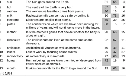
The two sets of data analysed are summarised in Table 1, with grey highlighting indicating the correct
answers. In the first half of the table are the ten biotechnology items from the 2002 Eurobarometer on
public perceptions of biotechnology. These are followed by the thirteen general science literacy items
posed in the 2005 Eurobarometer on Public Understanding of Science (PUS). In both surveys the
questions were posed to respondents in the then fifteen EU member states. Two key characteristics of
the data should be noted at this point. One is that some items are answered correctly by only a few
respondents, while others are answered correctly by many. The other is that ‘don’t know’ (DK)
Table 1 Distribution of responses to knowledge questions across fifteen EU countries
No. Label Statement % responses2
True False DK
Knowledge about biotechnology, 2002
1 bacteria There are bacteria which live from waste water. 84 3 12 2 tomato Ordinary tomatoes do not contain genes, while
genetically modified tomatoes do.
35 36 29
3 clone The cloning of living things produces genetically identical copies.
66 16 18
4 fruit By eating a genetically modified fruit, a person’s genes could also become modified.
20 49 31
5 mother It is the mother’s genes that determine whether a child is a girl.
23 53 24
6 yeast Yeast for brewing beer consists of living organisms. 63 14 23 7 test It is possible to find out in the first few months of
pregnancy whether a child will have Down’s Syndrome.
79 7 14
8 animal Genetically modified animals are always bigger than ordinary ones.
27 38 35
9 chimpanzee More than half of human genes are identical to those of a chimpanzee.
52 15 33
10 transfer It is not possible to transfer animal genes into plants. 29 26 45
n=16,040
Knowledge about science in general, 2005
1 sun The Sun goes around the Earth. 31 65 4
2 hot The centre of the Earth is very hot. 87 6 6
3 oxygen The oxygen we breathe comes from plants. 80 15 4
4 milk Radioactive milk can be made safe by boiling it. 10 75 16
5 electrons Electrons are smaller than atoms. 45 30 25
6 plates The continents on which we live have been moving for millions of years and will continue to move in the future.
88 5 7
7 mother It is the mother’s genes that decide whether the baby is a boy or a girl.
20 65 15
8 dinosaurs The earliest humans lived at the same time as the dinosaurs.
22 67 11
9 antibiotics Antibiotics kill viruses as well as bacteria. 40 49 11
10 lasers Lasers work by focusing sound waves. 26 47 27
11 radioactivity All radioactivity is man-made. 27 60 13
12 human Human beings, as we know them today, developed from earlier species of animals.
72 19 9
13 month It takes one month for the Earth to go around the Sun. 19 65 16
n=15,518
2 Weighted frequencies, weighting each country’s contribution to the total according to their respective population sizes. Totals
Methods for scaling
The typical approach to creating a scale from these items is to add up the number of correct
responses. This simple sum-score approach is potentially problematic in a number of ways, however.
Firstly, it does not allow for any measurement error in the items. Secondly, it does not allow the
possibility of distinguishing between a substantively incorrect response and a DK response. Thirdly, it
usually means assigning equal weights to all items in the scale, even though some are more diagnostic of people’s knowledge than other items.
In these sets of items, it would be beneficial to address the three concerns. Firstly, it is well
understood, both in educational testing and in attitude research that items are imperfect indicators of
the concepts that we try to capture using them. Secondly, it can be informative to distinguish between
a DK response and substantive response, in order to investigate possible response effects in the data,
that is, particular types of measurement error. DK response rates are very high in both item sets
analysed in this chapter, and particularly for the biotechnology items. Thirdly, it would make sense to
award credit to items differently, depending on their content, just as would be done in a typical
examination or test.
In the analyses below I use latent trait models to address these three concerns (for an introduction,
see Bartholomew et al. 2008). So I hypothesise the existence of a construct, ‘science knowledge’,
which cannot be directly observed, and take answers to the individual survey questions as imperfect
manifestations of that latent variable. If the items all tap into the construct, then they should be
statistically associated with each other; these associations should be explained by the latent variable ‘knowledge’. Latent variable models in general can be thought of most simply as regression models
with multiple observed response variables and a smaller number of unobserved explanatory variables.
It may be the case, with these knowledge items, that more than one latent variable, more than one
unobservable attribute, is required to adequately explain the patterns of responses to these questions.
Perhaps, by way of illustration, the responses that are given to these items are best explained by two
latent variables, one of which captures levels of knowledge, and the other which picks up a certain response style which influences people’s answers but separately from their level of knowledge. An
expected response style might be, for example, acquiescence bias – that is the tendency to agree or give a positive response to questions – which is often found in survey data.
Latent variable models enable us to address the three current concerns in the following ways. Firstly,
they allow for measurement error by specifying a probabilistic rather than a deterministic relationship
between item responses and the latent variables that explain them. Secondly, particular latent variable
models can be employed that enable us to retain the distinction between substantive and DK
responses. In survey research latent variable models are most commonly applied in the form of factor
analyses based on linear regression models, which assume that latent variables and observed items
are continuous, interval-level variables. However, these are inappropriate when observed items are
categorical, which is clearly the case with the items to be analysed, and indeed is often the case
they define logistic regressions for the relationship between categorical item responses and
continuous latent traits. Latent trait models are better known in some fields as Item Response Theory
(IRT) models (van der Linden and Hambleton 1997). In the models presented in this paper, my first
approach is to treat the observed knowledge items as three-category nominal items, that is essentially
to use a multinomial logit model for the relationship between each item and the latent trait(s).
Lastly, the question of determining whether some survey items should receive more or less weight in a scale of knowledge, and exactly what weights, can be addressed using the model’s parameter
estimates. Latent trait models provide a number of useful pieces of information about a set of items.
For each item (or item category, if there are more than two categories) the slope coefficient or loading
tells us to what extent the item (or category) enables us to discriminate between respondents on the
trait; the higher the loading, the greater the discrimination, the more pertinent the item is to the substance of the trait, the greater its weight should be in determining a person’s position or ‘score’ on
the trait. Items with high discrimination power will help us to capture ‘knowledge’ and to calibrate
respondents in terms of their levels of knowledge. Items that have low discrimination power do little
work for us in characterising respondents, and may be candidates for deletion from future survey
waves. Alongside discrimination parameters, the model specifies constants or intercepts. Whereas
these are not of great interest in the linear factor model, in latent trait models they have heuristic value
when expressed as difficulty parameters for the items. The difficulty of a particular response is defined
as the probability of giving that response for the median individual on a trait. It is desirable to have
items with a range of difficulty levels in any one scale.
The combined information from item loadings and intercepts can be represented graphically, by
calculating a selection of fitted probabilities of item responses for a range of values for a latent trait
(fixing the other trait(s) at some values, if there is more than one trait – in this chapter, the other
trait(s) are fixed at their means when this is done). From such fitted probabilities we can draw Item
Characteristic Curves (ICCs) or trace lines, which show at a glance the changing probabilities of
choosing each of the response categories at any point along the latent trait. ICCs show for each item
its discrimination power, via the steepness of the slopes of its response curves (the steeper the slope,
the greater the discrimination), and its difficulty, by way of the location of the curve in the plot (the
higher on the latent trait, the greater the difficulty).
Jon Miller’s various analyses of the closed form knowledge items – both of the science literacy scale,
and of the Eurobarometer-style questions focusing on biotechnology-related facts – employ latent
variable models, and constitute the most advanced approach in the PUS literature, to my knowledge.
He takes binary items (where there are DK responses these are recoded as ‘incorrect’), uses a
preliminary factor analysis to identify items that form a unidimensional scale, then applies a
three-parameter logistic model to these items, that is with difficulty and discrimination three-parameters, and an
extra parameter to correct for guessing. Miller, Pardo and Niwa (1997) and Miller and Pardo (2000)
employ these models for comparative studies of the EU, US, Japan and Canada.
In this chapter I adopt a slightly different approach from Miller and colleagues to deal with possible
response effects. Since the literature suggests that a third, ‘guessing’ parameter is only weakly
identified (Skrondal & Rabe-Hesketh, 2004; Thissen & Wainer, 1982), and my samples are of
standard sizes (roughly a thousand in each country), I keep to a two-parameter logistic model, but
allow more than one trait to try to account for response effects. This is potentially advantageous not
only because of statistical identification reasons, but also because I suspect that there is a more
complex response style in the Eurobarometer items than guessing between two options. The data contain high rates of DK responses, and in the biotechnology items the ‘true=correct’ items tend to be
answered correctly more often than the ‘false=correct’ items. These data may therefore contain a
mixture of acquiescence bias, propensity to guess, and propensity to profess ignorance – in addition
to the knowledge we are trying to capture. So I retain the distinction between DK and an incorrect
response, use two-parameter logistic models and allow the possibility of needing more than one trait
to represent the variation in the data. Further, I model the latent traits as discrete, with seven levels,
rather than as continuous (see Heinen 1996). This has particular advantage that it does not impose
the assumption of a normal distribution for the latent trait, so we can allow for the possibility that
knowledge is not symmetrically distributed among the population.3
In order to address the question of cross-national comparability, I focus on differences and similarities between European countries in the construct ‘knowledge’ that can be derived from the items using
latent trait models. The logic is that if the estimated item parameters (loadings and difficulties) for a trait representing ‘knowledge’ are very different from country to country, then the relationships between the survey items and the construct ‘knowledge’ is different from country to country. This
would imply that in a statistical sense the items do not capture knowledge in the same way from place
to place. We should then be cautious when drawing comparisons between countries using these
items, and consider modifying them in future surveys towards the goal of creating broadly comparable
scales. If, however, the item loadings and difficulties can be constrained to be the same between
countries without compromising model fit too much, then we can reasonably speak of a common construct ‘knowledge’, and that it makes statistical sense to use it as a means of comparing levels of knowledge from country to country. Whether it also makes substantive sense is the next question –
and not for this chapter. The statistical approach here is roughly analogous to those applied to
continuous observed items in factor analysis, for which there are many more demonstrations and discussions of ‘non-equivalence’ or ‘invariance’ of item parameters in the literature (for a recent
example and overview see Allum, Read and Sturgis, forthcoming).
Procedurally, in this chapter I first of all find adequate models for knowledge for each country
separately. Then for each of these models I compare their parameter estimates informally. I then
attempt to find a single model across the whole data set, with country as a covariate, where the
loadings and intercepts are fixed to be the same for all countries. The criteria for ‘finding a model’ are those of model fit and model interpretation. In order to assess model fit I focus on two-way marginal
residuals, following Bartholomew et al. (2002), Bartholomew and Knott (1999) and Jöreskog and
3 Models are estimated using Latent GOLD (Vermunt & Magidson 2005). Item characteristic curves and some fit statistics are
Moustaki (2001).4 As well as fitting adequately, a model must make substantive sense. In this context,
at the most basic level it means that the odds of answering questions correctly should increase as one moves up the latent trait ‘knowledge’.
Results of scaling the biotechnology knowledge items
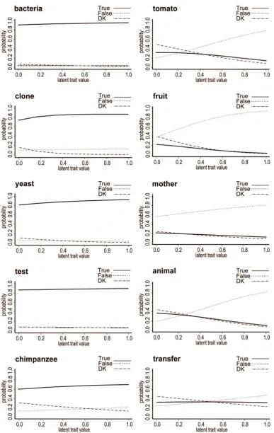
By way of orientation, I present here the results from a two-trait model for the ten items in the British
sample, which fits the data well (2.7 per cent of standardised marginal residuals > 4). Figure 1 shows the ICCs of what I label the ‘knowledge’ trait for this model. Each plot refers to one of the items, with the value of the latent trait on the horizontal axis and the probability of giving the responses ‘true’, ‘false’ or ‘DK’ on the vertical axis. It can be seen that as one moves from the lower to the higher end of
this trait (from lower to higher levels of knowledge), broadly speaking, the probability of giving a
correct response increases, and the probability of giving an incorrect or a DK response decreases.
The other trait (which is less interesting and not presented here) seems to summarise the tendency to
give a DK rather than a substantive response – this is the response effect trait which I expected to
find.
This broad interpretation of the knowledge trait comes with two qualifications, however. Firstly, all
those items listed in the left hand side of the figure have very shallow slopes or low discrimination power: it hardly matters whether one is ‘low’ or ‘high’ on knowledge; the probability of giving a correct
response is very similar at every point. Moreover that probability is high: these items are easy to get
right; chimpanzee is the most difficult, but even for this item, a person at the lower end of the trait has around a 60 per cent chance of answering it correctly. So these items do not do a lot of ‘work’ for us in
helping to distinguish between people who have high versus low levels of knowledge. Notably, these items share the characteristic that ‘true’ is the correct answer. The items displayed on the right hand side, for which, incidentally, ‘false’ is the correct answer, generally have much greater discrimination
power: a person at the lowest end of the knowledge scale has about a 20 per cent chance of
answering the item tomato correctly, whereas a person at the highest end has about an 80 per cent
chance of giving the right answer. Note that tomato is a more difficult item than fruit (just below it); a
person with the median level of knowledge is more likely to answer fruit than tomato correctly.
The second qualification to the general interpretation is that a few of the slope estimates suggest a
problematic interpretation. The signs of the true and false slopes for clone and chimpanzee are
actually in the wrong order: the probability of giving the incorrect response (for both items, ‘false’)
increases as the level of the trait increases. The slope estimates for ‘true’ and ‘false’ responses on
these two items are actually not significantly different from each other (at p<0.05). However, the
implication of the model for the calculation of posterior scores (‘factor scores’) for the trait is that a person answering all other items correctly but incorrectly saying ‘false’ to these two items would be
4For responses to each pair of items, I create a two-way marginal table, by collapsing over responses to the other variables. I
assigned a slightly higher score than a person answering all items correctly. Under this model, the
[image:9.595.84.472.156.769.2]former has a score of 0.943 and the latter, 0.917.
Figure 1 Item characteristic curves for the ‘knowledge’ trait from a 2-trait discrete trait
The next step in fitting a model to the British data would be to drop the problematic items from the
scale, in order to find a model in which the slope coefficients are aligned in the directions which fit
logically with a scale defining high knowledge at one end. This exercise is in fact quite problematic.
Removing items from the scale noticeably destabilises the items remaining – most notably, the ‘true=correct’ items, making it difficult to find a model in which the slope coefficients take the required
signs. Within the scope of the several models that I attempted, I could not find one which represented
any improvement over the ten item scale, especially in terms of producing factor scores that were
logically ordered according to numbers of correct answers. So the ten item trait remains the final
model for this section on the British sample, but with a caveat attached to it.
Moving on to the explore a joint model of knowledge items for the fifteen countries, separate
country-by-country analyses suggest that two-trait models are a feasible starting point. Using all ten items in
the set, two traits fit well for all country samples: the percentage of large two-way standardised
marginal residuals ranges from 0.2 in Finland to 7.2 in Germany, with a mean of 2.4 per cent across the fifteen countries. In all countries, one trait can be reasonably labelled ‘knowledge’, while the interpretation of the other trait varies a little more between samples – of the range of interpretations, the most common is a response effect trait, with DK responses at one end, and ‘false’ at the other.
Focusing on the ‘knowledge’ trait, Table 2 gives a qualitative summary of the few items and few countries for which slope coefficients deviate from the pattern to be expected in a trait capturing knowledge. It reflects the model of the British data, in that many of the ‘true=correct’ items lack
discrimination power in some countries, and in a number of cases, whilst the overall probability of a
correct response is highest at the highest point of the trait, the slope for the incorrect response is increasing – implying the problems with factor scores encountered in the British data. However, these
are not such a serious problem compared with the last item, transfer, for which in five countries, at the ‘high knowledge’ end of the trait the probability of giving the incorrect response is greater than the
probability of giving the correct response. In these cases it is very clear from the ICCs that the item
does not fit logically with the others in the scale. From this point it is dropped from the item set.
Repeating these exploratory analyses with nine items leaves the qualitative summary of them in Table
Table 2 Qualitative summaries of unusual Item Characteristic Curves (ICCs) on biotechnology ‘knowledge’ traits, from 2-trait models, 15 countries
‘True=correct’ items ‘False=correct’ items
bacteria clone yeast test
chimp-anzee tomato fruit mother animal transfer
Austria
Belgium d d, c-, i+
Denmark c-, i+ i+ I, c-, i+
Finland c-, i+ i+
France c-, i+ c-, i+ c-, i+ c-, i+
Germany c-, i+ c-, i+ c-, i+ i+ I, i+
Greece i+ i+
Ireland i+ i+ c-, i+
Italy c-, i+ c-, i+ c-, i+ c-, i+
Luxembourg d d d, i+ I, d
Netherlands d d d d I, d
Portugal i+ I, i+
Spain c-, i+ c-, i+ c-, i+ I, i+
Sweden d d
UK d d i+ d
Key
d Low discrimination: very flat ICCs
c- Slope for correct response decreasing slightly with higher levels of ‘knowledge’ i+ Slope for incorrect response increasing slightly with higher levels of ‘knowledge’ I ‘Incorrect’ most likely response at top end of trait
regular font Slight effect
bold font Strong effect: more seriously problematic
From the example of ICCs given in Figure 1 it is clear that some items have greater discrimination
power than others. In a joint trait model, the relative discrimination of the items would be fixed to be
the same between countries. Unfortunately, it seems that the differences in ICCs between countries
are too large for a joint trait model, with the same measurement model for each country, to fit well.5 In
the joint version of the two-trait models for nine items, 42 per cent of standardised two-way marginal
residuals are large. The number of large residuals is notably high for four items: tomato, yeast, animal
and chimpanzee, in terms of two-way item-by-item margins as well as country-by-item margins, and
three-way item-by-item margins. Dropping these from the scale almost halves the proportion of high
residuals, but the rate is still 26.3 per cent. Increasing the number of traits also helps model fit: a
three-trait model with these four problematic items removed reduces the proportion of high residuals
to 15.9 per cent. This is still arguably too high (compare for example with the latent class models in
5 As a brief preliminary analysis for such a joint model, an indicative analysis was carried out, focusing on item discrimination
power, defined as the discrimination parameters of correct in comparison with incorrect responses – that is, ignoring the slope estimates for DK responses, for the moment. If the discrimination parameters of certain pairs of items were in a significantly different order in different countries – say, if tomato were more highly discriminating than bacteria in some countries, but less highly discriminating than bacteria in others – it would be a clear sign that finding a well fitting joint model would be difficult. The analysis was carried out with S-Plus software, using 95 per cent confidence intervals around the differences between slope estimates, and applying the Bonferroni correction to allow for multiple comparisons. In fact, only two pairs of items (bacteria with yeast and tomato) appear to have significantly different relative discrimination powers, and then, only between Portugal and
Spain, for the first pair, and Portugal versus Spain and Denmark, for the second.5 This gives grounds for optimism that a
Mejlgaard and Stares, this volume). Moreover, the measurement of knowledge from these items is
considerably unstable. In the models with equal measurement models between countries for all traits,
I found that different numbers and combinations of items produced quite different solutions – echoing
the findings from the two-trait model of British data presented as an example. Some combinations of items failed to return a trait successfully representing correct ‘knowledge’ at one end, even when the model contained three traits. So although these items are intended to constitute a sample from a wide universe of knowledge items, the interpretation of the construct ‘knowledge’ seems to depend, more
than is desirable, on the combination of items contributing to it.
Since the objective for this model is to derive a measurement of knowledge, there should be no
compromise to the model by allowing the second trait, which fills the role of accounting for response
styles, to differ between groups. That is, a feasible joint model might be one with a fixed trait representing ‘knowledge’, and a country-specific trait for response effects. However, for this set of
items, it does not provide a solution. Both with nine items, and with a reduced set of five items
(chosen by means of inspecting large two-way and three-way marginal residuals, as above), the fixed trait cannot be interpreted as ‘knowledge’. It seems to be closer to a response effect, with DK and one end and ‘false’ at the other, regardless of whether this is the correct response. Albeit these models
represent a great improvement in fit (13.2 per cent large two-way residuals for the nine-item model for example), they do not return a viable representation of ‘knowledge’.
From these analyses, then, it seems that finding a viable joint model for these items is a difficult task.
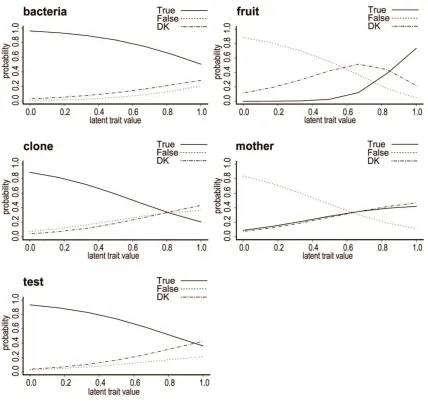
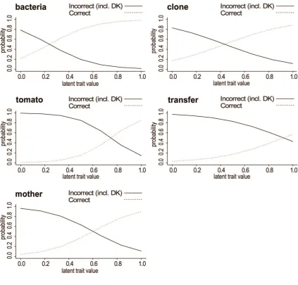
The models attempted here either fit badly or do not identify a trait that could feasibly be interpreted as ‘knowledge’, and seem to be numerically unstable. Out of the models presented in this section, the three-trait model with five items is the best representation of ‘knowledge’, cross-nationally. The ICCs for the ‘knowledge’ trait from this model are presented in Figure 2. Note that for this trait low scores
Figure 2 Item characteristic curves from 3-trait discrete trait models for 3-category
nominal items, with measurement models equal for all traits, for 15 countries,
biotechnology ‘knowledge’ trait
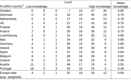
Having decided on the best cross-national scale that can be derived from these items, the question
follows to ask how knowledge is distributed country-by-country. Table 3 shows the distribution of
levels of knowledge according to this trait (reversed from the original model so that high levels of the
trait denote high levels of knowledge). Specifically it shows the percentage of the population estimated
to belong at each of the seven levels of the trait, by country, and for the fifteen countries together,
weighted by their respective populations. Countries are ordered from highest to lowest mean
knowledge score. The distribution of the trait among countries is consistent with expectations from the
PUS literature: high levels of knowledge are found among the Northern European countries, and with
some exceptions, lower levels among those in the South. Overall, Europeans score quite highly on
this scale, with very few people falling into the lower three levels of the trait, and with an EU wide
Table 3 Percentages of respondents in each level of the final joint model of
biotechnology knowledge items
% within country6 Low knowledge
Level
High knowledge
Mean knowledge
Sweden 0 0 0 7 10 47 36 0.85
Denmark 0 0 0 16 15 45 23 0.79
Netherlands 0 0 0 17 15 44 22 0.78
UK 1 0 1 22 17 42 18 0.75
Finland 1 0 1 30 19 36 12 0.70
France 2 0 1 30 19 36 12 0.70
Luxembourg 2 0 1 31 19 35 11 0.69
Italy 4 1 1 34 19 32 9 0.66
Germany 4 1 2 36 19 30 9 0.65
Ireland 5 1 2 36 18 30 9 0.65
Spain 5 1 2 37 19 29 8 0.64
Belgium 6 1 2 38 18 28 8 0.63
Greece 8 1 2 43 18 23 5 0.59
Austria 11 2 3 46 17 19 4 0.55
Portugal 18 2 3 45 15 15 3 0.49
Europe total 4 1 1 32 18 33 12 0.68
(pop. weighted)
Given the lack of success in finding a well fitting joint model for the polytomous items, the question
naturally arises whether the difficulties with the models above are due to retaining the distinction
between DK and substantively incorrect responses. Since it is much more common to model binary
versions (correct versus incorrect, with DK counted as an incorrect answer) in the PUS literature, I
briefly present the results of analyses of binary items here.
Country-by-country analyses suggest that one trait is sufficient to represent the data: percentages of
large two-way marginal residuals range from 0 in five countries, to 3.9 in Spain, and with a mean of
2.10, and all items take loadings of the same sign. The country-by-country models may be
qualitatively similar, but their parameters are different enough to make a joint model, fixing the
measurement model between countries, fit very poorly (43.1 per cent large two-way marginal
residuals). As before, both deleting problematic items from the scale, and increasing the number of
traits, improves fit dramatically. With five items, 26.3 per cent of two-way marginal residuals are large.
Notably, a somewhat different set of items are retained here in comparison with the model for polytomous items – in particular, transfer is included in the scale. A two-trait model for this set of items
improves the fit further (14.2 per cent large residuals), but with flat response curves for three of the
five items, it is of questionable value, and might be interpreted as a case of over-fitting. The one-trait
model for five items is therefore arguably the preferred model, all things considered. ICCs for it are
shown in Figure 3. It is interesting that correct responses to the item transfer are predicted to belong
to only those at the very top of the scale.
Figure 3 Item characteristic curves from a 1-trait discrete trait model for binary items,
with measurement models equal for 15 countries
Results of scaling the general science knowledge items
Speculating on possible causes of the problems encountered with the biotechnology items, their
content might be something to consider. Since in different models it was different items which caused
the problems with fit, it seems not to be the case that odd question wording in a few places is to
blame. Carrying out a similar set of analyses on the science literacy items therefore provides a useful
point of comparison.
The analyses here are somewhat truncated, for reasons of space. Modelling items as polytomous,
and running two-trait discrete trait models, country-by-country analyses identify a few items as
problematic, as with the biotechnology items: the signs of some item loadings on a country’s
‘knowledge’ trait return a counterintuitive interpretation. Deleting some items from the scale is therefore necessary step. Based on informal analyses of the kind summarised in Table 2, nine items
A two-trait model for these nine items, with equal measurement models between countries on both
traits, fits poorly – although notably, not as poorly as the two-trait nine-item model for the
biotechnology items (cf. 28.1 per cent large two-way marginal residuals for the former, versus 41.8 per
cent for the latter). Reducing the number of items in the scale does very little to reduce the proportion
of large two-way marginal residuals. However, a great improvement in fit is obtained by relaxing part
of the measurement model: namely, allowing both slopes and intercepts to vary between countries on
one trait, while constraining slopes to be equal across countries (with intercepts free to vary between
countries) on the other. In this model only 4.1 per cent of two-way marginal residuals are large, and
the fixed trait can feasibly be interpreted as representing low to high knowledge. Figure 4 shows ICCs
for this model, for UK respondents – that is, with the fixed, Europe-wide slopes but UK-specific
intercepts.
There are a few points to note here. Firstly, the slopes for correct responses are relatively steep, for
all items, compared with those in the biotechnology set (cf. Figure 1). That is, the science items
broadly speaking have greater discrimination power than the biotechnology items. Secondly, it is not
the case for the science items that all of the ‘false=correct’ items are more difficult than the ‘true=correct’ items. The first three items in the diagram, in the left hand column, are those for which ‘true’ is the correct response. The second, ‘Electrons are smaller than atoms’, is a relatively difficult
Discussion: implications for future survey design
The results of these analyses suggest that deriving a statistically comparable scale of knowledge across the fifteen European countries, using the items available, is a difficult task – and more so for
the biotechnology than for the science literacy items. However, the models also point quite clearly to a
number of modifications that might be considered in designing future surveys that include these kinds
of items.
Considering first of all the internal workings of the scale within countries, the most striking feature of
the knowledge items is that many of them are relatively easy, and therefore not diagnostic, as the
majority of respondents answer them correctly. However, it may not be that the items straightforwardly test facts that are very widely known. Those items for which ‘true’ is the correct response are easier (that is, more people answer them correctly) than those for which ‘false’ is correct. This could be an
indication that the high rates of correct answers are attributable to response effects such as guessing,
or acquiescence bias.
The biotechnology items and the science literacy items are similar in this regard, though the problem
is more acute for the biotechnology items. In their methodological analysis of the science items, Pardo
and Calvo (2004) suggest that the scale could be improved by adding or substituting more difficult
items in the set. They specifically recommend using more ‘false=correct’ items to increase the
difficulty level of the test. They also suggest offering a four-point Likert answer scale, to allow respondents to differentiate between whether they think each statement is ‘definitely’ or ‘probably’ true
or false, to alleviate guessing or other response effects. However, I would take a different approach.
Response styles such as acquiescence bias and guessing are known to be more likely among certain demographics, including cultural groups (Smith, 2003). Increasing the number of ‘false=correct’ items
might therefore lead the scale to favour a particular type of respondent, making it even more open to
charges of bias. The very odd scaling behaviour of the item transfer, which requires a double negative
for a correct response, is a good warning against over-using this strategy.
It would undoubtedly be useful to try to increase the number of difficult items, but this would be more
effective if it could be ensured that it was the content of the item, not the required response, which
was difficult. So it would be advantageous if these more difficult questions were mixed, with some requiring ‘true’ and some ‘false’ as correct responses. The four-point Likert response scale may to some extent reduce the possible effects of guessing and acquiescence bias, but a more likely
successful strategy might be to remove the true versus false dichotomy from the exercise altogether,
instead asking respondents to choose between the two. Many of the original science literacy and
biotechnology knowledge scale items could easily be reformulated in this style. For example, It is the mother’s genes that determine the sex of the child would become a task of choosing between the
statements It is the mother’s genes.. and It is the father’s genes... Multiple choice items might also be
considered. For example, the statement, Ordinary tomatoes do not contain genes, while genetically
modified ones do, could be reformulated as a question, such as:
A. Human beings
B. Fruits and vegetables
C. GM fruits and vegetables
D. A and B
E. B and C
F. All of the above.
Ideally the order of the first three response options would also be rotated. Multiple choice questions
are more complex to analyse, and more costly to field, but should be seriously considered as a
possible way of alleviating the response effects in the data.
Changing the item format altogether is a relatively drastic move: new items may always work less well
than established ones, and new items prevent the analysis of trends over time. A more moderate
strategy would be to add more difficult items to the existing set for the next survey, and evaluate the
effectiveness of this before considering changing the question format altogether in future waves.
Given the greater success in finding an adequate model for the science literacy items than the
biotechnology items, steering the content of these questions towards general science and away from
specific applications, such as biotechnology, might be advisable.
Adding items to an existing set seems to carry a smaller risk of failure than moving wholesale to a
different question format, but even with this approach, due consideration needs to be given to
respondent fatigue and the relative importance of this construct versus the other topics that need to be
covered in a given questionnaire. The matter requires a strategic decision by the survey designers. If
a model could be found to fit the items in their current format, this may be the best solution to creating a measure of knowledge. The two-trait model (with one fixed ‘knowledge’ trait and one free ‘response effect’ trait) which fits the science literacy items is an example of such a model. However, using more
than one trait, in order to account for response effects, such a model might not be as intuitive to a lay
audience as a unidimensional knowledge scale.
On a more positive final note, remember that in within-country analyses, the existing two-trait models
deliver a good deal of useful information about the items. For cross-country comparisons, given the
importance of knowledge to the PUS research field, more efforts to improve the scale would be
valuable. Methodological critiques of biotechnology and science knowledge scales emphasise this.
Pardo and Calvo (2004) point out that the weak association often found between measures of
knowledge and attitudes might be partly attributable to the quality of the scales used. In their
meta-analysis of the relationship between knowledge and attitudes, Allum et al. (2008) find the greatest
variance in their model attributable to the measures used, and very little to cross-national differences.
References
Allum, N., Read, S. and Sturgis, P. (forthcoming) Evaluating change in social and political trust in Europe using multiple group confirmatory factor analysis with structured means. In Davidov, E., Billiet, J. and Schmidt, P (eds) Methods for cross-cultural analysis: basic strategies and applications. Taylor and Francis.
Allum, N., Sturgis, P., Tabourazi, D., & Brunton-Smith, I. (2008). Science knowledge and attitudes across cultures: a meta-analysis. Public Understanding of Science 17(1). 35-54
Converse, P. E. (2000). Assessing the capacity of mass electorates. Annual Review of Political Science(3), 331-353.
Durant, J., Evans, G., & Thomas, G. (1989). The public understanding of science. Nature, 340, 11-14.
Heinen, T. (1996). Latent class and discrete latent trait models: Similarities and differences. Thousand Oaks, California: Sage.
van der Linden, W. J., & Hambleton, R. K. (Eds.). (1997). Handbook of Modern Item Response Theory. New York: Springer-Verlag
Miller, J. D. (1998). The measurement of civic scientific literacy. Public Understanding of Science, 7, 203-223.
Miller, J. D., & Pardo, R. (2000). Civic Scientific Literacy and Attitude to Science and Technology: A Comparative Analysis of the European Union, the United States, Japan, and Canada. In M. Dierkes & C. von Grote (Eds.), Between Understanding and Trust: the Public, Science and Technology.
Amsterdam: Harwood Academic Publishers.
Miller, J. D., Pardo, R., & Niwa, F. (1997). Public Perceptions of Science and Technology: A Comparative Study of the European Union, the United States, Japan, and Canada. Madrid: BBV Foundation.
Pardo, R., & Calvo, F. (2004). The cognitive dimension of public perceptions of science: methodological issues. Public Understanding of Science, 13, 203-227.
Peters, H. P. (2000). From Information to Attitudes? Thoughts on the Relationship between Knowledge about Science and Technology and Attitudes Toward Technologies. In M. Dierkes & C. von Grote (Eds.), Between Understanding and Trust - the Public, Science and Technology.
Amsterdam: Harwood Academic Publishers.
Shen, B. S. P. (1975). Scientific Literacy and the Public Understanding of Science. In S. Day (Ed.),
Communication of Scientific Information. Basel: Karger.
Skrondal, A., & Rabe-Hesketh, S. (2004). Generalized latent variable modeling: multilevel, longitudinal and structural equation models. Boca Raton, FL: Chapman & Hall/CRC.
Smith, T. W. (2003). Developing Comparable Questions in Cross-National Surveys. In J. Harkness, F. van de Vijver & P. P. Mohler (Eds.), Cross-Cultural Survey Methods. Hoboken, NJ: Wiley.
Stares, S. (2009) Using latent class models to explore cross-national typologies of public engagement with science and technology in Europe. Science, Technology and Society, 14(2), 289–329.
Sturgis, P. and Allum, N. (2004) Science in society: re-evaluating the deficit model of public attitudes.
Public Understanding of Science, 13, 55-74.
Thissen, D., & Wainer, H. (1982). Some standard errors in item response theory. Psychometrika, 47, 397-412.