Evolutionary neurocontrol: A novel method for low-thrust gravity-assist trajectory optimization

Evolutionary Neurocontrol: A Novel Method for Low-Thrust

Gravity-Assist Trajectory Optimization

Ian Carnelli

∗

ESA, 2001 AZ Noordwijk, The Netherlands

Bernd Dachwald

†

DLR, German Aerospace Center, 82234 Oberpfaffenhofen, Germany

and

Massimiliano Vasile

‡

University of Glasgow, Glasgow, Scotland G12 8QQ, United Kingdom

DOI: 10.2514/1.32633

The combination of low-thrust propulsion and gravity assists to enhance deep-space missions has proven to be a remarkable task. In this paper, we present a novel method that is based on evolutionary neurocontrollers. The main advantage in the use of a neurocontroller is the generation of a control law with a limited number of decision variables. On the other hand, the evolutionary algorithm allows one to look for globally optimal solutions more efficiently than with a systematic search. In addition, a steepest-ascent algorithm is introduced that acts as a navigator during the planetary encounter, providing the neurocontroller with the optimal insertion parameters. Results are presented for a Mercury rendezvous with a Venus gravity assist and for a Plutoflyby with a Jupiter gravity assist.

Nomenclature

^

er = sun–spacecraft unit vector

g0 = Earth’s standard gravitational acceleration

Isp = specific impulse J = fitness function

_

mp = propellant massflow

N = network function R = rotation matrix

S = spacecraft steering strategy

T = thrust vector

^

t = thrust unit vector

u = spacecraft control vector

v1 = hyperbolic excess velocity

xs=c = spacecraft staters=c;vs=c

= sphere of influence scaling factor

= thrust clock angle

= aiming point distance on theBplane

= thrust cone angle

= orbit inclination

= gravitational constant

= number of reproductions

= chromosome/individual

= population of chromosomes/individuals/pilots = network internal parameters vector

= throttle factor [0, 1]

= evolutionary neurocontroller

Subscripts

pl = assisting planet

1 = before the gravity-assist maneuver 2 = after the gravity-assist maneuver

Superscript

* = optimal

I.

Introduction

G

RAVITY assists (GAs) have proven to be the key to interplanetary high-energy missions. They not only make missions feasible that would otherwise be impossible due to large propellant mass fractions, but flybys also make missions more interesting for the scientific community. Additionally, low-thrust (LT) propulsion systems make interplanetary missions more efficient and moreflexible, allowing larger launch windows [1]. Hence, the combination of low-thrust propulsion and gravity assists (LTGA) provides an excellent means to reduce propellant mass-fraction requirements.

However, the design of such trajectories is no trivial task. The spacecraft control function on low-thrust arcs is a continuous function of time, and therefore the dimension of the solution space is infinite. The problem is further complicated by considerations of the planet’s phasing, especially when multiple gravity assists are sought. Finally, preliminary analysis tools such as the Tisserand plane or Lambert’s method are not applicable to LT trajectories.

The complexity of the solution of a multiple-LTGA (MLTGA) problem derives from the complexity of the simpler multiple-gravity-assist (MGA) problem. It should be noted that this complexity is not simply due to the hybrid nature of the MLTGA problem. It can be easily shown that even formulating the MGA problem in a homogenous fashion, with continuous decision vari-ables as in thefixed-sequence case, it retains its inherent complexity [2]. This is due to the following reasons: the MGA problem presents a high number of local minima, this number grows with the number of gravity maneuvers, the number of minima further increases if multiple revolutions or deep-space maneuvers are inserted between two subsequent planetary encounters, and the most interesting solutions are generally nested (i.e., their basin of attraction is narrow

Received 5 June 2007; revision received 6 October 2008; accepted for publication 8 October 2008. Copyright © 2008 by the authors. Published by the American Institute of Aeronautics and Astronautics, Inc., with permission. Copies of this paper may be made for personal or internal use, on condition that the copier pay the $10.00 per-copy fee to the Copyright Clearance Center, Inc., 222 Rosewood Drive, Danvers, MA 01923; include the code 0731-5090/09 $10.00 in correspondence with the CCC.

∗_{Systems Engineer, Advanced Concepts Team, European Space Research}

and Technology Centre, Keplerlaan 1; [email protected]. Member AIAA. †_{Scientist; currently Professor, Aachen University of Applied Sciences,}

Aerospace Engineering Department, Hohenstaufenallee 6, 52064 Aachen, Germany. Member AIAA.

‡_{Lecturer, Aerospace Engineering Department. Member AIAA.} Vol. 32, No. 2, March–April 2009

615

and generally falls within or near a wider basin of attraction of a worse solution).

Some of these reasons are related to the mathematical formulation of the problem and can be mitigated with an appropriate approach. For example, if no deep-space maneuvers are considered and the GA maneuvers are modeled through a powered-swingby model, it can be proved that the MGA problem is solvable incrementally in polynomial time, with a small exponent, through a simple branch-and-prune procedure [3].

Others are instead intrinsically related to the physical nature of the problem. In fact, in a MGA trajectory, the outgoing leg from a GA maneuver is highly sensitive to the incoming conditions. This sensitivity narrows down the size of the basin of attraction in comparison with a direct transfer. Furthermore, the ratio between the orbital periods of the planets tends to destroy any periodicity or symmetry in the solution space.

Despite what could seem intuitive, adding low-thrust arcs to a MGA trajectory does not change the global nature of the solution space. The main reason is that low-thrust arcs (in particular, when the solution is optimal) are only locally shaping each trajectory leg, tuning the entry conditions to a GA maneuver at a lower cost than deep-space maneuvers. This is true unless a multispiral trajectory is inserted between two gravity maneuvers. In this case, low-thrust arcs increase the complexity of the problem. Furthermore, if deep-space maneuvers and an accurate gravity-assist model are considered, the number of possible states for an MGA trajectories grows exponentially with the number of GA maneuvers, even for afixed sequence. The MLTGA problem therefore inherits the complexity of the MGA problem and adds the local solution of an optimal control problem.

Traditionally, the design and analysis of interplanetary LTGA trajectories undergoes three main steps:

1) The main objectives are selected and the sequence offlyby bodies is outlined.

2) Possible preliminary trajectories are analyzed. 3) The optimal trajectory is calculated.

Thefirst two steps, typically carried out by an expert in trajectory optimization, generate the initial guess for the third optimization phase. Unfortunately, this approach is typically quite inefficient, as each individual problem has to be solved from scratch and many solutions have to be explored before convergence of the optimization method is achieved. Finally, even if a solution is obtained, in most cases it represents a local optimum far from the global optimal solution. Recent studies have attacked the problem using either deterministic (such as branch and prune) or stochastic global optimization methods (such as evolutionary algorithms) [4–8].

Though the use of stochastic-based methods allows the treatment of high-dimensional problems that are otherwise intractable with deterministic problems, modeling the control law through either an indirect approach or through direct collocation could not be the most efficient choice in the preliminary phase of the design.

It is proposed here to use evolutionary neurocontrollers (ENCs) instead, which have proven to be able to generate very good solutions to quite complex problems in an effective and efficient way. The ability of ENCs tofind, for example, optimal solar photonic assist trajectories to reach the outer solar system with a solar sail was demonstrated by Dachwald [9]. The proposed ENCs are veryflexible because they perform a broad search of the solution space without any special requirement on the regularity of the optimization function and of the constraints. They also allow one to accommodate the cooptimization of additional problem parameters (e.g., launch date, hyperbolic excess velocity, etc.).

If we consider the usual classification of the methods for trajectory design [10], the evolutionary neurocontroller would fall in the class of direct approaches in particular, because the dynamics here are propagated forward in time, in the class of direct shooting methods. This basic classification, however, does not help to understand the essence of the evolutionary neurocontroller. The main difference with respect to the other direct methods is that the neurocontroller generates a time-dependent control law, as for indirect methods, with a low number of decision variables. The advantage can be

understood through a simple example: If a multispiral trajectory were to be designed and the number of spirals were not known a priori, a direct shooting methods based on a collocation of the controls would require an increase of the number of decision variables as the number of spirals increases to have a good resolution of the control profile. A neurocontroller would instead require a constant, and small, number of control variables. We can say that as neural networks can be used to map a generic nonlinear function, the neurocontroller can also be used to map a generic controller.

In this paper, we present a novel method to design LTGA trajectories that is based on ENCs. This new tool is an extension of InTrance (Intelligent Trajectory Optimization Using Neuro-controller Evolution), the global LT trajectory-optimization tool developed by Dachwald [11].

II.

Simulation Models

Some general assumptions are used throughout this paper to simplify the models and to relax the computational effort:

1) Along a low-thrust arc, the spacecraft is subject to the gravity attraction of the sun and to the control acceleration of the engine only. Gravity-assist maneuvers are inserted between two low-thrust arcs as hyperbolic trajectories in the planetocentric reference frame. Finally, along the gravity-assist hyperbola, the spacecraft is subject to the gravity attraction of the GA planet only.

2) The magnitude and direction of the spacecraft’s thrust vector can be achieved instantaneously.

3) The spacecraft systems (e.g., solar arrays, electric thrusters, etc.) do not degrade over time.

InTrance implements several solar sail models, two solar electric propulsion (SEP) systems (NASA’s NSTAR thruster and QinetiQ’s T6 thruster), and a nuclear electric propulsion (NEP) system. The preliminary results presented in this paper make use of the NEP system for the Plutoflyby mission and the (NSTAR) SEP system for the Mercury rendezvous mission.

A. NEP System Model

In this model, the maximum thrustTmaxand the specific impulse

Ispare assumed to befixed. The maximum propellant massflow rate

_

mp;max(required to generateTmax) is

_

mp;max jTmaxj

jvej

jTmaxj

Ispg0

(1)

where ve is the exhaust velocity and g0 is Earth’s standard gravitational acceleration. A throttle factor01 is used to control the propellant massflow rate, so that

_

mp m_p;max (2) and

T Tmaxm_p;maxIspg0 (3) whereT jTj. Thus, propellant massflow rate and thrust vary only with. In contrast to SEP systems, the thrust is independent of solar distance, which makes the NEP especially suited for missions to the outer solar system. Using the thrust unit vector^tto denote the thrust direction, Eq. (3) then becomes

T Tmax^tm_p;maxIspg0^t (4)

B. SEP System Model

The key parameter for a SEP system is the input powerPPPUthat is available to the power processing unit (PPU). This power is proportional to that delivered by the solar arrays PSA (which is 1=r2_{, whererrepresents the solar distance). The available power}

PAVmust also take into account the power required to operate the spacecraft’s systemsPSYS:

PAVr PSA

1

r2

PSYS (5)

For the NSTAR engine, a throttle01is used to control the PPU power input, so thatPPPUis defined as

PPPU; r

8 < :

0 ifPAVr< Pmin

PAVr ifPminPAVr Pmax

Pmax ifPAVr> Pmax

(6)

wherePminandPmaxrepresent the minimum and maximum power at which the propulsion system can operate (respectively, 0.5 and 2.0 kW). According to Williams and Coverstone-Carroll [12], the following polynomial approximation for the propellant massflow rate (in milligrams/second) and thrust (in millinewtons) can be used in the power rangePminPPPUPmax:

_

mp; r

1 mg=s0:74343

0:20951PPPU

1 kW

0:25205P2 PPU

1 kW2 (7)

T; r

1 mN 3:4318

37:365PPPU

1 kW (8)

The minimum and maximum massflow rate and thrust are then

_

mp;min0:9112 mg=s m_p;max2:1707 mg=s

Tmin15:251 mN Tmax71:298 mN Finally, the expression for the specific impulse is

Isp; r

jT; rj

_

mp; rg0

(9)

III.

Equations of Motion for EP Spacecraft

When a spacecraft employs chemical thrusters to generate the requiredV, the maneuvers can be considered to be impulsive, due to the high level of thrust and consequently short burning times. However, if a spacecraft uses electric propulsion, the burning times are comparable with the spacecraft’s orbital period, and hence the thrust has to be included within the equations of motion. Therefore, the differential equations system is

_

rv v_

r2e^r

T

mSC

(10)

wheree^ris the unit vector pointing from the attracting bodyBtoward the spacecraft, andGM_B is the gravitational constant. Using Eq. (4), one gets for NEP

rTmax mSC

^

t

r2e^r (11)

_

mSC m_p;max (12) whereas for SEP spacecraft,

rT; r

mSC

^

t

r2e^r (13)

_

mSC m_p; r (14) The orientation of the thrust unit vector_t^(expressed by the thrust clock angleand the thrust cone angle) and the throttleconstitute the spacecraft’s control vector: that is,uu; ; .

IV.

Gravity-Assist Model

Labunsky et al. [13] proposed an analytical method that allows an approximate computation of gravity assists. We have implemented this method into InTrance to avoid direct numerical integration of the equations of motion within the assisting body’s sphere of influence (SOI). This way, the required computation time is reduced con-siderably. Nevertheless, this method provides a quite accurate description of the gravity-assist maneuver.

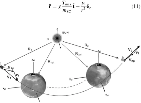
Given the spacecraft statexsc rsc;vscon the SOI before the gravity-assist maneuver, the purpose of this method is to provide the spacecraft state on the planet’s SOI after the gravity assist. The spacecraft’s position and velocity in the heliocentric reference systemfR1;V1gwhen entering the SOI, as well as those of the planet fRpl;1;Vpl;1g, are supposed to be known (see Fig. 1). According to the SOI approximation, the coordinate system is changed into the planetocentric reference frame. The spacecraft’s state thus becomes

r1R1Rpl;1 (15)

v1V1Vpl;1 (16)

wherejr1j RSOI;pl, the subscript 1 indicates a variable before the gravity-assist maneuver, and the subscript pl is used to indicate a variable of the assisting planet. From the planetocentric point of view, the spacecraft approaches from infinity with a nonzero velocity. Therefore, the trajectory is represented as hyperbolic, and the outbound velocity and position vectors result from a rotation around the angular momentum vectorhscwith respect to the planet (see Fig. 2). The outbound state of the spacecraft is then obtained using

x2

y2

z2

0 @

1

AR

x1

y1

z1

0 @

1

A (17)

vx2

vy2

vz2

0 @

1

AR’

vx1

vy1

vz1

0 @

1

A (18)

where is the rotation angle of the position vector,’is the rotation angle of the velocity vector, and R is a rotation matrix. The complementary angles are given by

’2 ’22 arctan v2

1

(19)

where

arccosr1v1

jr1jjv1j

andv1

v2 12=r1

p

represents the hyperbolic excess velocity. Finally, is the aiming point distance defined as the distance between the center of the planet and the inbound asymptote: Fig. 1 Schematic diagram of the gravity-assist maneuver.

[image:3.585.45.282.569.742.2]

RSOI;plsin (20) Of course, must be chosen so that the trajectory’s resulting pericenter radius is greater than the radius of the assisting planet, including the height of its atmosphere,rp>Rplhatm. Finally, to perform the gravity-assist computations, R is defined as in Appendix A.

V.

Low-Thrust Trajectory Optimization Using

Evolutionary Neurocontrollers

The LTGA trajectory-optimization problem is attacked from the perspective of artificial intelligence and machine learning. In this context, a trajectory can be regarded as the result of a spacecraft steering strategySthat maps the problem-relevant variablesX2X onto the spacecraft control vectoru2U:

S:X fxsc;xT;xpl;i;xscxT;xscxpl; mpg !U fug

wherexpl;i (i2npl) refers to the state of allnplpotential gravity-assisting bodies andmpis the actual propellant mass. Note that time is not explicitly a problem-relevant variable, because independent of time, the same constellation of planetary bodies requires the same steering vector. This way, the problem of searching the optimal spacecraft trajectory is equivalent to the problem of searching for (or learning) the optimal steering strategyS?_.

An artificial neural network (ANN) is used as a so-called neurocontroller (NC) to implement such spacecraft steering strategies. It can be considered as a parameterized function N (called network function) that is completely defined by the set of the network’s internal parameters2Rn_{. This way, eachde}fi_{nes a}

steering strategy S. The problem of searching for the optimal

spacecraft trajectory is thus equivalent to the problem of searching for the optimal parameter set?_{, given a neurocontroller topology.} Here, only feedforward ANNs are considered, in which neurons are organized hierarchically in three layers: namely, the input , hidden, and output layers [9]. Every neuron implements a sigmoid transfer function [11]. Every neuron in the input layer accepts one component ofXas input, and the output layer consists of three neurons providing the spacecraft control vector uu; ; . The middle layer comprises 30 neurons, though the number of neurons in this layer generally has little effect on the optimality of the final steering strategy that the NC represents.

Evolutionary algorithms (EAs) that work on a population of strings can be used tofind the optimal network parameters because they can be mapped on a string(also called a chromosome or individual). The trajectory-optimization problem is then solved when the optimal chromosome?_{is found. Figure 3 summarizes the} subsequent transformations of the optimal chromosome into the optimal trajectory. A neurocontroller that employs an evolutionary algorithm to learn the optimal control strategy is referred to as an evolutionary neurocontroller. Evolutionary operators that are tailored to work on real-valued strings and neural networks have

been used: namely, one-point crossover operator, uniform crossover, crossover nodes, and mutation [11]. The quality of the solution and, even more so, the search duration depend on the population size. A good compromise between these two factors was found by selecting a population size of 50 individuals, the quality of the solution being quite insensitive to the actual number. A more detailed description of the implemented EA is beyond the scope of this paper and can be found in [11].

A. InTrance

The ENC architecture used in this work is sketched in Fig. 4. This particular ENC design reflects its application to solve LT trajectories optimization problems. To do so, the ENC runs in two loops. Within the inner trajectory-integration loop, a NC steers the spacecraft according to its network functionNprovided by the EA (that runs in

the outer loop). The NC’s parameter set , which represents an individual, is therefore constant during integration. It can be thought of as a pilot who steers the spacecraft until the termination condition is met. That is, the pilot has either reached the final target or a maximum travel time (defined by the user). In the outer optimization loop, the EA holds a population f1;2;. . .;qgof pilots (or chromosomes/individuals). The EA evaluates all pilots (i.e., NC parameter sets j2f1;...;qg), one at a time, for their suitability to generate an optimal trajectory. Within the trajectory-optimization loop, the NC takes the actual spacecraft statexsctiand that of the target bodyxTtias input values and maps them onto the output values from which the spacecraft control vector uti can be calculated. At this point, xscti and uti are inserted into the equations of motion, which are numerically integrated over one time steptti1tito yieldxscti1. This state is fed back into the NC. Again, the trajectory-integration loop stops when the termination condition is met. At this time, the NC’s parameter set (i.e., its trajectory) is rated by the EA’sfitness functionJj. This fitness value is crucial to the reproduction probability ofj. Under the selection pressure of the environment, the EA breeds NCs that generate increasingly suitable steering strategies (offspring) that in turn generate increasingly better trajectories. The EA that is used within InTrancefinally converges to a single steering strategy that gives, in the best case, a globally optimal trajectoryx?

sct. B. Objective Function

The optimality of a trajectory can be defined with respect to different (primary) objectives such as transfer time or propellant consumption. When an ENC is used for trajectory optimization, the trajectory accuracy to the terminal constraints must also be considered as a secondary optimization objective, as they are not explicitly stated elsewhere. By defining a maximal allowed distance

rf;max and relative velocityvf;max at the target, the trajectory accuracy can be defined as follows with respect to the terminal constraints:

Xf

1 2R

2 fV

2 f

q

(21) Fig. 2 Schematic diagram of the gravity-assist maneuver.

Fig. 3 From chromosome to optimal trajectory.

[image:4.585.79.241.44.194.2] [image:4.585.353.504.573.748.2]

where

Rf

rf

rf;max and

Vf

vf

vf;max

In the beginning of the search process, most individuals do not achieve the required accuracy, and hence a maximum transfer time

Tmaxmust be defined for the numerical integration of the trajectory. The subfitness functions

JTc1

1 T

Tmax

Jmp

mpt0

c2mpt0 mptf

c3 (22)

(we have chosenc11000,c22, andc31=3) for the primary optimization objectives have been found to work well and the subfitness functions

Jrlog

1 Rf

Jvlog

1 Vf

(23)

have been defined for the secondary optimization objectives.Jrand

Jvare positive if the respective accuracy requirement is fulfilled and they are negative if it is not. The values of the constants are arbitrary and do not influence the selection probability or the optimization result, because a tournament-selection procedure is used, in which the selection probability is independent of the scaling of the subfitness functions and thefitness function [11]. Simulations have showed that the search process should first concentrate on the accuracy of the trajectory and then on the primary optimization objectives. Therefore, the subfitness functions for the primary optimization objectives are modified to

J0 T

0 ifJr<0 or Jv<0

JT ifJr0 and Jv0

J0 mp

0 ifJr<0 or Jv<0

Jmp ifJr0 and Jv0

Therefore, to minimize the transfer timeT for a rendezvous, the following function is used:

JT;rf;vf J0T

1

c4 1c4Xf

(24)

(we have chosenc40:99), whereas to minimize the propellant consumptionmp, thefitness function is similar, butJ0Tis replaced withJ0

mp:

Jmp;rf;vf J0mp

1

c4 1c4Xf

(25)

A tournament-selection scheme has been used for the selection of the individuals from the population [11]. This way, the selection probability does not depend on the scaling of thefitness function. The value chosen forc4guarantees that once thefinal constraints are fulfilled, improvements in the primary optimization objective are rated much higher than improvements in the fulfillment of thefinal constraints (but if two individuals have the same flight time or propellant consumption, the more accurate one is always preferred). In the case of a planetaryflyby, only the constraint on the position must be met, whereas thefinal velocity is set free. If the transfer time is to be minimized in this case, then

JT;rf J0mp

1

c4 1c4Rf

(26)

To minimize the propellant mass for aflyby,J0

Tis replaced withJ0mp:

Jmp;rf J0mp

1

c4 1c4Rf

(27)

VI.

ENC Architecture Options

Two different approaches to solve the LTGA problem are straightforward. In one case, the whole trajectory (i.e., the inbound leg from the departure point to theflyby body and the outbound leg from theflyby body to the target body) is optimized by a single NC. This choice is quite straightforward, as it requires only the input to the ANN and the chromosome length to be modified, but it preserves the structure of the EA operators. However, in such an approach, there is no objective evidence that the ENC will actually seek for gravity-assist maneuvers and exploit them to gain orbital energy (only some expectations based on the ENC ability to perform solar photonic assists for solar sail trajectories [14]).

A second approach instead requires the use of multiple ENCs. Here, each ENC optimizes only a single leg of the trajectory. In other words, the mission is divided into sequential phases: thefirst phase starts from the departure body and ends at the SOI of thefirstflyby body. The gravity-assist maneuver at this moment is computed analytically to give the outbound conditions (subscript 2), then the second leg is optimized by a second ENC until the next SOI or the final target body is reached. This reasoning can be extended ton1

ENCs (_j2f1;...;n1g) performingngravity-assist maneuvers. Atfirst sight, this second approach seems very promising because InTrance has proven to be capable offinding optimal?

j. By creating new

evolutionary operators and providing aflyby sequence, one can be quite confident of finding the optimal overall trajectory for this sequence?

1 ?n1. Although the latter approach is quite

attractive, it fails in one particular point that is the goal of this work: designing a fully automatic tool that does not require the attendance of a trajectory-optimization expert. If theflyby sequence were to be given as an input to InTrance, either an expert or a second ad hoc algorithm would have to provide it. For this reason, the single-ENC approach has been chosen.

VII.

Gravity-Assist Optimization

Within the single-ENC approach, thefirst step is to provide the ENC with the appropriate input information. This corresponds to the knowledge the ENC should have to optimally steer the spacecraft and eventually perform gravity assists. In addition to the state of the spacecraft and thefinal target, the ENC should also know where the possible gravity-assist bodies are and how they are moving. In other words, the NC’s inputs must include additional information such as

xscxpl.

The second step is to introduce the analytical gravity-assist calculator into the inner trajectory-integration loop of the ENC. Here, a patched-conics approximation is used: at every integration step, a Fig. 4 Evolutionary neurocontrol architecture.

[image:5.585.53.272.46.198.2]

check is performed to determine whether the spacecraft has entered the SOI of a gravity-assist body. If this is the case, the maneuver is calculated analytically and the outbound conditions (subscript 2) are used as initial conditions for the successive numerical integration, which is carried out until the termination condition is met.

Finally, the third step corresponds to the gravity-assist maneuver optimization. To do so, theBplane, which can be thought of as a target attached to the assisting body, is taken as reference system.§

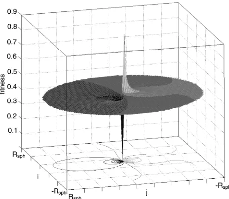
The topology of the solution space for the optimal planetary maneuver was assessed by plotting thefitness values corresponding to a large-enough number of targeting pointsx; yon theBplane for one exemplary gravity assist. Once a grid is defined on the plane, some virtual spacecraft were used to probe the solution space by forcing them to aim at each grid point. This way, a sufficient subset of all possible maneuvers was tested and rated with respect to thefitness function. Following this procedure, a plot can be made in which thex

andyaxes correspond to theB-plane coordinates, and thezaxis (the height of the surface) corresponds to thefitness valueJx;y. Figures 5 and 6 show that the solution space for this exemplary gravity assist is particularly smooth and regular (here, the Venus gravity assist of the test case in Sec. VIII is used).

For this exemplary gravity assist, the two extremes (i.e., the absolute maximum and the absolute minimum) are very well defined, and only a local minimum and maximum are present on the boundary of the SOI, because of the slight inclination of thefitness plane toward the positivexaxis. A few characteristics of the solution space are noteworthy:

1) As the gravity-assist geometry is incorporated in the neurocontroller’s steering strategy (that is fixed once a neuro-controller is selected because its parameters are constant), each ENC can onlyfly one of the many possible GA geometries. Thus, theB

plane corresponds to afixed point in space with a frozen incoming velocity vector (only the thrust profile may vary before and after the GA, but not the geometry of theflyby) characterized by a solution space with a single optimum.

2) The two global extremes are symmetrically located with respect to the origin and separated by about the diameter of the planet. There is in fact only one semi-Bplane that bends the spacecraft trajectory toward the target body, hence boosting the spacecraft in the right direction. Also, the two extremes are close to theflyby body in which its gravitationalfield is strongest and the trajectory’s curvature is most affected.

3) The solution space in the outer regions is almostflat. This is also an expected result because the maneuvers performed close to the SOI

boundaries (outer region of the equatorial circular plane in Fig. 5) have small effect on the trajectory.

4) No other hills or valleys are found in the domain. This suggests adopting a local optimization method rather than a global optimizer for the maneuver, for the sake of saving computing time. This simple structure of the solution space, however, might not generally be the case. Especially if multiple gravity assists are involved, a global method might offer advantages.

5) In this particular case, the fitness values are in the range

0<J<0:9(note thatJ1corresponds to fulfillment of thefinal constraints), but the values close to the optimum are located in a very small region of the domain space.

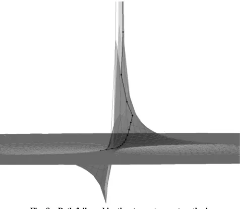
Following the preceding analysis, we have chosen a steepest-ascent method as the optimization algorithm. The goal is tofind the highestfitness-function value: that is, the highest rewardJthat can be attributed to the navigator. Because local optima are present only in the outer regions of the SOI, there is no risk of converging to a local optimal solution if the initial pointxi; yiis chosen to be close enough to the planet. The strategy, which consists of following the path along the steepest gradient, is illustrated in Fig. 7. Using this simple algorithm, an efficient navigator for the ENC is designed. The best gravity-assist maneuverx; y?_{is located within a few iterations} (see Fig. 8) and is so efficient that the fitness of individuals that perform a gravity assist far outweighs thefitness of the individuals who do not.

The gravity-assist maneuver is performed when the spacecraft reaches the SOI of an assisting body. Here, the trajectory integration is stopped and the spacecraft’s velocity vector defines the orientation of theBplane. At this stage, the actual aiming pointr1is disregarded and the coordinate setx; y? _{optimized by the navigator is used} instead. This pointr1is projected onto the SOI to provide the initial Fig. 5 Two-dimensional plot ofB-planefitness topology.

Fig. 6 Three-dimensional plot ofB-plane topology.

Fig. 7 Search algorithm.

§_{It is a planar coordinate system that contains the focus of the hyperbola}

and is perpendicular to the incoming asymptote. The origin of the reference system is the center of the assisting body, thexaxis is defined by the intersection of theB plane with the trajectory plane, and theyaxis is orthogonal to thexaxis.

[image:6.585.309.540.45.246.2] [image:6.585.44.279.46.220.2] [image:6.585.305.546.612.742.2]

position for the analytical gravity-assist calculator. The discontinuity that is introduced is minimized during the optimization process. This is done by introducing the distancejr1r1jin a subfitness function

Jdistance

1

jr1r1j

that is to be maximized once the primary goal is achieved [Jr0and

Jv0, as defined in Eq. (23)]. Finally, the gravity-assist maneuver is computed and the initial conditions for the following trajectory leg are obtained.

Because of the modest size of the SOIs, the chances for an ENC to encounter a sphere of influence are very small. To solve this problem, artificial spheres of influence are introduced to enlarge the real SOI sizes (with the exception of Jupiter and Saturn) by a factor >1. The idea is to let the ENC learn in an easier environment and gradually raise the difficulty by letting !1 while the number of reproductions in the population increases. Empirically, the following definition of was found to provide a good learning environment to the ENC:

1600:5

400:5 if <600

1 if600

The 600th-generation threshold is chosen to provide the ENC with the real dynamic environment, typically after the primary goals are achieved and before the secondary goals are optimized. Note that the number of generations required is problem-dependent. However, no LTGA optimization problem was found to require less than3000

generations.

VIII.

Test Cases

The algorithm defined in the previous section proved to be an efficient navigator for the ENC. The idea is to let the ENC (pilot) concentrate only on the trajectory-optimization task and support each pilot with a navigator whom he can consult whenever a SOI is crossed. Two missions are used as a reference to assess the validity of this method: aflyby mission to Pluto with a Jupiter gravity assist and a rendezvous mission to Mercury with a Venus gravity assist. The first mission is somewhat easier due to the very large size of Jupiter’s SOI. The second mission is much more challenging due to the demandingVrequirement to reach Mercury.

A. New Horizon Mission to Pluto

The proposed approach was implemented in an extended version of InTrance called InTrance-GA. To assess its ability to optimize LTGA trajectories, aflyby mission to Pluto calculated by Vasile [8]

was chosen as a reference. In that paper, the design of the NEP trajectories was performed with a direct transcription method based onfinite elements in time (implemented in a software tool called DITAN [15,16]). However, because the problem presents a number of possible solutions dependent on the launch window and transfer time, a global optimization strategy was used [8] to generate sets of promising initial guesses. By setting the launch date and escape velocity to those used in the reference and the terminal conditions so that the arrival at Pluto is before 2020, InTrance-GA could generate results that are comparable with the so-calledfast transit optionin the reference. This was most probably achieved due to a very short integration step (i.e., one day). Thus, the objective of this simulation was not to optimize the launch conditions andfind a global optimum solution, rather to explore the local level of accuracy that can be reached once a solution is found. The results summarized in Table 1 were obtained by evolving an initial population size of 50 individuals for 1367 generations, requiring a total computation time of 23,795 s and reaching anfitness-function value ofJ33:77. As can be seen, there is very good agreement between the two solutions. In particular, the propellant mass consumptions are nearly identical (the NEP model described in Sec. II.A. was used). Note that InTrance-GA was able achieve a very good local convergence so that virtually no refinement of the solution was needed. However, a minimumfinal flyby distance at Pluto as high asrf1e6 kmwas reached and could not be further minimized, whereas Jdistance 1755 km1 was considered sufficiently low to consider the overall solution to be accurate.

B. Mercury Rendezvous

As a second test case to assess our method’s performance, a rendezvous trajectory to Mercury, as calculated by Debban et al. [17] and De Pascale [18], was chosen. This optimization goal is particularly challenging for several reasons, including Mercury’s proximity to the sun and the eccentricity and inclination of its orbit. Even assuming circular coplanar orbits of both Earth and Mercury, a Hohmann transfer requires a launchV1of at least7:5 km=s, with the resulting arrivalV1 as high as9:6 km=s[19]. The idea of using chemical propulsion to remove this hyperbolic excess velocity is prohibitive, and hence LTGA techniques offer lower propellant requirements.

In the paper by Debban et al. [17], the whole computational effort is focused on the search for a proper initial guess [using the Satellite Tour Design Program (STOUR)-LTGA, a shape-based method that implements exponential sinusoid functions], which is then optimized using a direct method (implemented in a software tool called GALLOP). The chosen trajectory shape is a two-dimensional curve in polar coordinates. Here, the target’s out-of-plane position at the time of the in-plane encounter is matched by using additional thrust acceleration acting along or against the spacecraft’s angular momentum vector for somefinal portion of the leg’s thrust arc. By assuming constantIsp, the propellant consumption is then estimated as a fraction of the initial spacecraft mass based on the time integral of the thrust acceleration and the rocket equation. Finally, the effect on the time offlight (TOF) is neglected. Thus, the trajectory along thez

[image:7.585.42.280.46.253.2]

coordinate is well approximated only for small inclination changes. An evolution of this method (implemented in a software tool called IMAGO) by De Pascale [18] describes the trajectory by assigning a Fig. 8 Path followed by the steepest-ascent method.

Table 1 Earth–Jupiter–Pluto mission with NEP

DITAN InTrance-GA

Earth launch date 19 January 2006 19 January 2006

LaunchV1 12 km=s 12 km=s

Mass at departure 600 kg 600 kg

Mass at arrival 565.5 kg 565.3 kg

Isp 3000 s 3000 s

Thrust 40 mN 40 mN

Jupiter encounter 23 February 2007 4 March 2007 Pluto arrival 4 October 2014 13 October 2014

[image:7.585.317.533.662.755.2]

set of shapes to a set of so-called pseudoequinoctial elements, allowing a fully three-dimensional description. These methods provide interesting results to assess the performance of InTrance-GA.

The obtained results, together with the reference values, are shown in Table 2. Here, the SEP model as described in Sec. II.B was used, and the launch conditions were optimized over the following ranges: the launch date was between 15 June 2002 and 15 September 2002 and the launchV1range was set between 2 and3 km=s. There is good agreement between InTrance-GA and IMAGO over the launch date, time offlight, and arrival date. The different SEP, trajectory model, and wider range of variability of the initialV1might instead justify the difference with GALLOP. InTrance-GA was able to rendezvous with Mercury after 2842 generations, requiring a total computation time of 41,484 s, which once again demonstrates the complexity of this rendezvous problem. Afinal fitness value of J973:4was reached, though thefinal rendezvous values were somewhat relaxed torf;max5e5 kmand vf;max300 m=s. Once again,Jdistanceproved to be an easier parameter to minimize, and a fairly low value of1230 km1_{was reached.}

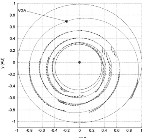
Figure 9 shows the trajectory found by InTrance-GA. The ENC manages to use the gravity-assist maneuver to obtain an initial orbit-inclination change(the scale on thezaxis is exaggerated for the sake of visibility). The remaining inclination change_♀is carried out by the spacecraft’s electric propulsion system. In addition to two correction maneuvers, thefirst immediately after departure and the second slightly before the Venusflyby, all thrust phases work to achieve the required orbit-inclination change.

The thrust and coast arcs can be better seen from Fig. 10, which provides a view from above the ecliptic plane, and from the spacecraft’s throttle level shown in Fig. A1. Note that there are no clear switching points and the thrust is continuously throttled from 0 to its maximum. The solution is therefore expected to be locally suboptimal. Nevertheless, it represents a goodfirst guess for this transfer trajectory.

IX.

Conclusions

We have presented a novel method (termed InTrance-GA) for low-thrust gravity-assist trajectory optimization, which is based on the use of evolutionary neurocontrollers. Based on an enumerative analysis of the solution space in theBplane, a separate algorithm was

implemented to optimize the gravity-assist maneuvers. This steepest-ascent algorithm acts as a navigator that the neurocontroller consults whenever it enters the sphere of influence of an assisting planet. Also, we have introduced artificially enlarged spheres of influence, due to their small size as compared with typical trajectory radii. This allows the evolutionary neurocontroller to learn in an easier environment, while gradually raising the difficulty by reducing the size to the real dimensions over time.

[image:8.585.109.476.60.136.2]

Preliminary results for a Plutoflyby with a Jupiter gravity assist and for a Mercury rendezvous with a Venus gravity assist have been presented. They show excellent agreement between the calculated solutions and the reference trajectories. In particular, in one of the Table 2 Earth–Venus–Mercury rendezvous trajectory

GALLOP IMAGO InTrance-GA

Earth launch date 13 August 2002 1 July 2002 9 July 2002

LaunchV1 1:93 km=s 3:0 km=s 2:99 km=s

Propellant mass fraction 0.310 0.3 0.314

Isp N/A 3300 s 3300 s

Earth–Venus TOF 198 days 183 days 154 days

Total TOF 853 days 936 days 1019 days

[image:8.585.305.546.293.525.2]

Fig. 9 Earth–Venus–Mercury trajectory and thrust vector (z-axis scale exaggerated).

[image:8.585.304.540.559.742.2]

Fig. 10 Mercury rendezvous trajectory from above the ecliptic plane.

Fig. A1 Spacecraft’s thrust history.

[image:8.585.43.284.592.736.2]

cases, InTrance-GA was able to perform a global search of the solution space in a way that required virtually no further refinement of the solution.

Appendix A: Gravity-Assist Model

The rotation matrixR, necessary to calculate the gravity-assist maneuver, is obtained by successive rotations: afirst set of rotations transforms the Cartesian coordinate system into the polar orbital reference frameOdefined by the three orthogonal unit vectorse^_r,e^_t, ande^_h, wheree^_ris along the radial sun–spacecraft direction,e^_his along the spacecraft’s orbital angular momentum vector, and the orbit transversal vector is e^_te^_he^_r. The peculiarity of this reference frame is that thee^_taxis changes constantly along the orbit. In other words, the anglebetweene^_tande^_’equals the inclination of the orbit only at the nodes, whereas it is null at right angles. The value of this angle can be obtained using the spacecraft velocity vector expressed in polar coordinatesvr; v’; v#:

arctanv#

v’

(A1)

Thus, the first set of rotation matrices that transforms from the Cartesian into the polar orbital reference frame is obtained by three subsequent rotations aboute^,e^’, ande^r. It follows that

Rpol;orbRr0 R’#0 R#’0 (A2) where’0and#0represent the azimuth and elevation of the spacecraft at the moment it enters the SOI:

’0arctan

y

x #0arctan z

x2_y2

p (A3)

Once the reference frame is set to the polar orbital, the second rotation is the one that actually carries out the maneuver. Hence, the velocity and position vectors are rotated about the orbital angular momentum vectore^h by, respectively, angles’and defined by Eq. (19) through the rotation matrix R^_e

h. Finally, a third set of

rotations is used to bring the reference system back to Cartesian. These rotation matrices can be easily obtained by transposing Eq. (A2):

RcartRT

pol;orb Rr0 R’#0 R#’0T RT

#’0 R T

’#0 RTr0 (A4)

All the subsequent rotation matrices have now been defined and the final expression for the overall rotation matrixRin Eqs. (17) and (18) can be provided:

R RcartR^_eh Rpol;orbR

T #’0 R

T

’#0 RTr0

R^_eh Rr0 R’#0 R#’0 (A5)

R’ RcartR^_eh’ Rpol;orbR

T

#’0 RT’#0 RTr0

R^_eh’ Rr0 R’#0 R#’0 (A6)

Using Eqs. (17) and (18) together with Eqs. (A5) and (A6), the spacecraft’s planetocentric Cartesian state after the maneuver is defined. Its components can be added to those of the assisting planet to define the spacecraft’s location and velocity at the moment it leaves the SOI in the heliocentric ecliptic coordinate system:

R2r2Rpl;2 (A7)

V2v2Vpl;2 (A8)

where subscript 2 is used to indicate a variable after the gravity assist has occurred (i.e., at timettpl), and Rpl;2 and Vpl;2 can be computed using the osculating elements of the body and the duration of the maneuver. The time offlight for a hyperbolic orbit within the

SOI is defined as

tpl2

a3

s

sinhH

sin H

(A9)

whereHis the hyperbolic eccentric anomaly. Its value is determined by the semimajor axisaof the hyperbola, the semirotation angle, and the radiusRSOIof the SOI:

Hcosh1

1RSOI

a

sin

a

jv1j2

2

RSOI

1

(A10)

Acknowledgment

The authors would like to express their gratitude to Wolfgang Seboldt at DLR, German Aerospace Center, for alwaysfinding the time for suggestions and in-depth discussions.

References

[1] Racca, G. D.,“Capability of Solar Electric Propulsion for Planetary Missions,”Planetary and Space Science, Vol. 49, No. 14, Dec. 2001, pp. 1437–1444.

doi:10.1016/S0032-0633(01)00084-8

[2] Vasile, M., and De Pascale, P., “Preliminary Design of Multiple Gravity-Assist Trajectories,” Journal of Spacecraft and Rockets, Vol. 43, No. 4, 2006, pp. 794–805.

doi:10.2514/1.17413

[3] Izzo, D., Becerra, V. M., Myatt, D. R., Nasuto, S. J., and Bishop, J. M., “Search Space Pruning and Global Optimisation of Multiple Gravity Assist Spacecraft Trajectories,” Journal of Global Optimization, Vol. 38, June 2007, pp. 283–296.

doi:10.1007/s10898-006-9106-02003.

[4] McConaghy, T., Debban, T., Petropoulos, A., and Longuski, J., “Design and Optimization of Low-Thrust Trajectories with Gravity Assists,”Journal of Spacecraft and Rockets, Vol. 40, No. 3, 2003, pp. 380–387.

doi:10.2514/2.3973

[5] Hartmann, J.,“Low-Thrust Trajectory Optimization using Stochastic Optimization Techniques,”M.S. Thesis, Univ. of Illinois at Urbana– Champaign, Urbana, IL, 1996.

[6] Coverstone-Carroll, V., Hartmann, J., and Mason, W.,“Optimal Multi-Objective Low-Thrust Spacecraft Trajectories,”Computer Methods in Applied Mechanics and Engineering, Vol. 186, Nos. 2–4, June 2000, pp. 387–402.

doi:10.1016/S0045-7825(99)00393-X

[7] De Pascale, P., Vasile, M., and Ercoli Finzi, A.,“A Tool for Preliminary Design of Low Thrust Gravity-Assist Trajectories,” Space Flight Mechanics Conference, Maui, HI, American Astronautical Society Paper 04-250, Feb. 2004.

[8] Vasile, M.,“A Global Approach to Optimal Space Trajectory Design,” AAS/AIAA Space Flight Mechanics Meeting, Ponce, Puerto Rico, American Astronautical Society Paper 03-141, Feb. 2003.

[9] Dachwald, B., “Optimization of Interplanetary Solar Sailcraft Trajectories Using Evolutionary Neurocontrol,”Journal of Guidance, Control, and Dynamics, Vol. 27, No. 1, 2004, pp. 66–72.

doi:10.2514/1.9286

[10] Betts, J.,“Practical Methods for Optimal Control Using Nonlinear Programming,”Advances in Control and Design Series, Society for Industrial and Applied Mathematics, Philadelphia, 2001.

[11] Dachwald, B.,“Low-Thrust Trajectory Optimization and Interplan-etary Mission Analysis Using Evolutionary Neurocontrol,” Ph.D. Thesis, Univ. der Bundeswehr München; Fakultät für Luft- und Raumfahrttechnik; Inst. für Raumfahrttechnik, Munich, 2004. [12] Williams, S., and Coverstone-Carroll, V.,“Mars Missions Using Solar

Electric Propulsion,”Journal of Spacecraft and Rockets, Vol. 37, No. 1, 2000, pp. 71–77.

doi:10.2514/2.3528

[13] Labunsky, A., Papkov, O., and Sukhanov, K.,Multiple Gravity Assist Interplanetary Trajectories, 1st ed., Gordon and Breach, Amsterdam, 1998, pp. 10–15.

[14] Dachwald, B.,“Optimal Solar Sail Trajectories for Missions to the Outer Solar System,”Journal of Guidance, Control, and Dynamics, Vol. 28, No. 6, 2005, pp. 1187–1193.

doi:10.2514/1.13301

[15] Vasile, M., and Bernelli-Zazzera, F.,“Targeting a Heliocentric Orbit Combining Low-Thrust Propulsion and Gravity Assist Manoeuvres,”

Operations Research in Space and Air, Applied Optimization, Vol. 79, Kluwer Academic, Norwell, MA, 2003.

[16] Vasile, M., and Bernelli-Zazzera, F., “Optimizing Low-Thrust and Gravity Assist Manoeuvres to Design Interplanetary Trajectories,”

Journal of the Astronautical Sciences, Vol. 51, No. 1, Jan.–Mar. 2003, pp. 13–35.

[17] Debban, T., Mc Conaghy, T., and Longuski, J., “Design and

Optimization of Low-Thrust Gravity-Assist Trajectories to Selected Planets,”AIAA/AAS Astrodynamics Specialist Conference, Monte-rey, CA, AIAA Paper 2002-4729, Aug. 2002.

[18] De Pascale, P.,“Strumenti di Indagine Globale per la Progettazione Preliminare di Traiettorie Interplanetarie,”M.S. Thesis, Politecnico di Milano, Milano, Italy, 2003.

[19] Sims, J., “Delta-V Gravity Assist Trajectory Design: Theory and Practice,” Ph.D. Thesis, School of Aeronautics and Astronautics, Purdue Univ., West Lafayette, IN, 1996.