Abstract—The Hit-or-Miss transform (HMT) is a well known morphological transform capable of identifying features in digital images. When image features contain noise, texture or some other distortion, the HMT may fail. Various researchers have extended the HMT in different ways to make it more robust to noise. The most successful, and most recent extensions of the HMT for noise robustness, use rank order operators in place of standard morphological erosions and dilations. A major issue with the proposed methods is that no technique is provided for calculating the parameters that are introduced to generalize the HMT, and, in most cases, these parameters are determined empirically. We present here, a new conceptual interpretation of the HMT which uses a percentage occupancy (PO) function to implement the erosion and dilation operators in a single pass of the image. Further, we present a novel design tool, derived from this PO function that can be used to determine the only parameter for our routine and for other generalizations of the HMT proposed in the literature. We demonstrate the power of our technique using a set of very noisy images and draw a comparison between our method and the most recent extensions of the HMT.
Index Terms— Machine vision, Morphological operations,
Object recognition, Segmentation
I. INTRODUCTION
athematical Morphology, first introduced by Matheron [1] and Serra [2] and later extended by Heijmans [3], provides an extremely powerful set of tools for image processing. Among these is the HMT [2] and [3], which is capable of identifying groups of connected pixels that comply with certain geometric properties. If there is noise in a given image, or if image features are extremely textured, the standard HMT will fail to detect objects which are of interest.
For the processing of binary images, the HMT is well
Manuscript received April 16, 2010. Paul Murray is with the Department of Electronic and Electrical Engineering, University of Strathclyde, Glasgow, G1 1XW, UK (phone: +44 141 548 2205; fax: + 44 141 552 5781; e-mail: paul,[email protected]). Stephen Marshall, is with the Department of Electronic and Electrical Engineering University
of Strathclyde, Glasgow, G1 1XW, UK
(e-mail:[[email protected]]). EDICS TEC BIP
defined, [2]–[7], and involves searching an image for locations where predefined templates simultaneously fit the image. The templates, known as structuring elements (SEs) in morphology, are designed to match the geometry of objects of interest in the foreground and background of the image. If SEs are designed to closely match the geometry of the image features that are of interest, just one noisy pixel in the foreground or background can cause this transform to fail since the SEs will no longer fit as a result of the noise. To overcome these issues, various authors have proposed techniques that involve some pre-processing of the image or some modification of the SEs or of the HMT itself.
In [8], Zhao and Daut present a technique for the detection of imperfect shapes where the SEs are designed by first smoothing the original image using a morphological opening, before using the boundary of these smoothed shapes as SEs. In [9], the same authors present a technique which uses the skeletons of both the object to be recognized and its complement as SEs.
In [10], Bloomberg and Maragos introduce a Rank Hit-Miss Transform using rank order filters in place of erosions to improve the performance of the HMT and its robustness to noise. The same authors present a Blur Hit-Miss transform in [11] which uses “blur SEs” to dilate the foreground and background of the image prior to applying the respective erosions of the HMT. This helps remove noise and makes it easier for the SEs to match patterns by slightly modifying the geometry of features in a given image.
Various researchers have defined methods to extend the HMT for the processing of grayscale images and recently a unified theory for calculating a grayscale HMT has been presented in [12]. We review in this paper, the most prevalent extensions of the HMT for grayscale images and show the equivalences between these extensions. Despite the extensions of the HMT for processing grayscale images, the issues that cause the HMT to fail in the presence of noise in binary images, have the same effect in the grayscale case. Various techniques attempt to generalize the HMT for feature recognition in noisy images. In [13], Khosravi and Schafer present a formal definition of the grayscale HMT and analyze its performance in the presence of Gaussian and salt and pepper noise. To improve the performance of the HMT in noise, the authors generalize the HMT using rank order operators and also subsample the SEs used for
A New Design Tool for Feature Extraction in
Noisy Images based on grayscale
Hit-or-Miss Transforms
P. Murray* and S. Marshall
template matching.
More recently, in [14], Perret et al present a Fuzzy Hit-or-Miss Transform which they use to detect features in very noisy astronomical images. Their technique uses rank order operations and a large set of SEs that are generated using a mathematical model. The authors also highlight some techniques that could be used to improve the robustness of other grayscale HMTs when operating in noise. We too discuss these extensions and show how their parameters may be calculated using our design tool.
Each of the aforementioned methods and extensions aim to improve the performance of the HMT such that it is more robust for feature detection in noisy images. Rank order operators feature heavily in this work, however, there appears to be a conceptual gap in that the authors fail to provide a method by which it is possible to select the appropriate rank or threshold for applying rank order filters in this way. This paper presents a Percentage Occupancy Hit-or-Miss transform (POHMT) which allows partial fitting of SEs in a similar fashion to the partial fitting allowed by rank order filters. The difference here however, is that we also provide a technique to accurately determine the rank of the filter that must be used for the detection of objects of interest. Furthermore, as a direct result of the plots that we use as a design tool, we show in this paper, how we can make the POHMT operate as a discriminatory filter which allows objects to be selectively marked or discarded by the transform.
II. MATHEMATICAL MORPHOLOGY
We first recall here the definition of the binary HMT before reviewing the work of various researchers who have extended the HMT such that it can be applied to grayscale images. We then present a novel, conceptual definition of the HMT in terms of SE occupancy and use this to explain the inability of the HMT to function where images are distorted by noise or when features exhibit internal texture.
A. The Hit-or-Miss-Transform
The HMT of a binary image X is the intersection of an erosion of X and erosion of the complement of X by a complementary pair of SEs BFG and BBG respectively where
X, BFG and BBG are sets in 2D space,
2
E=ℤ . BFG and BBG
are defined relative to a common origin in E where the composite SE
FG BG
B=B ∪B and
FG BG
B ∩B = ∅. That is,
{
}
( ) | ( ) , ( ) c
B FG x BG x
HMT X = x∈E B ⊆X B ⊆X (1)
where
( ) {
|}
x
B = b+x b∈B and a feature is detected by the
HMT if there is at least one point
x
∈
E
such that the foreground SE (BFG)x is included in X whilst the backgroundSE (BBG)x is simultaneously included in its complement,
\ c
X =E X, see [2]-[7]. The HMT returns a “marker” consisting of single pixels or groups of pixels indicating the presence and locations of the objects that have the features specified by B. To recover the complete object after detection, an opening by reconstruction [7] may be applied.
Unlike other morphological transforms, extending the HMT for grayscale images is not a trivial task since the HMT is not an increasing transform [7], [12], [14]. Various researchers have proposed extensions of the binary HMT such that it can be applied to grayscale images. A thorough review of these techniques, as well as a unified theory for calculating the grayscale HMT is given in [12]. We present here a brief summary of the main extensions of the HMT, and further details can be found in [12] and [14].
To remain consistent with the literature, we define the notation used throughout this paper. Let E represent a two dimensional digital space ( 2
E=ℤ ) and E
T be the set of all graylevel functions from a subspace of E to T where
{
,}
T= ∪ +∞ −∞ℝ or T = ∪ +∞ −∞ℤ
{
,}
such that T is acomplete lattice with respect to the order “
≤
”. Let EI∈T , denote a grayscale image, and E
B T∈ denote a grayscale SE. We can then define the grayscale erosion and dilation of image I by the SE, B, where the erosion of image I is denoted,
(
I ΘB)
, and the dilation of I is denoted,(
I⊕B)
:for all
x
∈
E
,
(
)( )
minsupp( )(
(
)
( )
)
,FG FG
FG b B FG FG FG
I B x I x b B b
∈
Θ = + − (2)
(
)( )
( )
(
(
)
( )
)
supp
max .
FG FG
FG b B FG FG FG
I B x I x b B b
∈
⊕ = − +
(3)
The grayscale HMT uses a pair of foreground and
background SEs, , E
FG BG
B B ∈T , where the grayscale HMT defined by Ronse in [15], (denoted RHMT in [14]) using our notation becomes,
[ ]( )( ) ( )( ) ( )( )
(
)
( )*
,
. -
FG BG
FG FG BG
B B
I B x I B x I B x
RHMT I x = Θ Θ ≥ ⊕ ≠ +∞
∞
if otherwise
(4)
where * *
( )
: and ( )
BG BG BG
B E֏T B b → −B −b , i.e. the dual of
BBG.
In [7] and [16], Soille defines an unconstrained HMT (UHMT) using flat SEs, which ∀ ∈x E, returns the number of cross sections of a grayscale image, I, where
(
FG)
x
B fits
the cross section,CS It
( )
, and(
BG)
xB simultaneously fits the
complement of this cross section,
( )
t
CS I
∁ ,
[BFG,BBG]( )( )
{
( FG)x t( ) ( , BG)x t( )}
.UHMT I x =card t B ⊆CS I B ⊆∁CS I (5)
In [12], the authors extend the UHMT as written in (5), to allow grayscale SEs, such that,
[BFG,BBG]( )( ) max
{
( FG)( )(
BG*)
( ), 0 .}
UHMT I x = I BΘ x − ⊕I B x (6)
containing the result of foreground erosions when this condition is satisfied. Soille’s UHMT produces a graylevel image where the intensity of each pixel indicates the number of cross sections where both SEs fit the image i.e. the difference between the foreground and background erosions.
In [14], the similarity between Soille’s and Barrat’s grayscale HMT defined in [17] is shown, where Barrat et al.’s HMT (denoted BHMT in [14]) is written,
[BFG,BBG]
( )( )
(
*BG)
( ) (
FG)( )
.BHMT I x = I⊕B x − ΘI B x (7)
Clearly, this grayscale HMT closely resembles that of Soille’s given in [12]. The two differ however in that Soille’s HMT returns the difference between the foreground erosion and the background erosion where Barrat et al. return the difference between the background erosion and the foreground erosion. In Soille’s HMT, the higher the output value, the better the fit of the SEs. The opposite is true for the BHMT, and the equivalence of these two operators is shown in [14] as,
[BFG,BBG]
( )( )
min{
( )( )
, 0}
UHMT I x = − BHMT I x (8)
Khosravi and Schafer, in [10], present their grayscale HMT which requires only one SE, BFG, as,
[BFG]
( )( ) (
FG)( )
(
(
FG)
)
( )
.KHMT I x = ΘI B x − − Θ −I B x (9)
This definition is discussed in [14], where it is shown that the KHMT is in fact equivalent to the BHMT as shown in (10) and (11),
( )( ) ( )( )
(
( )
*)
( )[BFG] FG FG ,
KHMT I x = ΘI B x − ⊕I B x (10)
[BFG,BFG]( )( ).
BHMT I x
= − (11)
Each of the proposed methods can be used to extract the features of a grayscale scale image that match the geometry of both BFG and BBG, however, all of these techniques fail in
the presence of noise unless further modifications are made. All of these techniques are discussed further in [14] and a thorough review of the grayscale HMTs proposed by Ronse and Soille is given in [12]. In this paper we extend the definition of the grayscale HMT given by Soille in [7] since it is consistent with our conceptual description of the operation of the HMT.
B. A New Conceptual View of the Hit-or-Miss-Transform
Interpreting a grayscale image as a topographic surface allows the HMT to be considered as a translation of the two SEs in this 3D image space searching for places where they simultaneously fit the image to detect objects. In the various definitions of the grayscale HMTs given in Section II.A, the SEs are translated in the 2D space, and standard morphological operations are used to probe the image where these operators interact with the graylevel at each
pixel as shown in (2) and (3). In the 3D space, we must still translate the SEs to all points x∈Ein the 2D space, however, we may also consider the translation of SEs in the vertical direction. From an implementation perspective we may first translate the SE by a vector x such that the origin of the SE is coincident with an image pixel x,∀ ∈x E. Then, at each pointx∈E, the concept of a vertical translation of the SE may be implemented by interrogating in some way, (dependent on the operation) the image pixels that are coincident with the elements of the SE, ∀ ∈t T.
The grayscale erosion of the image foreground can be described conceptually as a process of translating BFG to a
point x∈E and raising the SE to the highest level t for which it is entirely beneath or fully occupied by the signal. By this interpretation, the erosion of an image at any point
x∈Eis equivalent to calculating the maximum level, t, for which the foreground SE, BFG, is fully occupied in the
image. For the foreground erosion, the SE is fully occupied if the intensity of all image pixels that are coincident with the elements of BFG is greater than or equal to t. We denote
by lFG(x), the maximum level, t, for which the SE is fully
occupied when its origin is at any pointx∈E,
( ) max
{
, ( )}
.FG FG
FG FG FG
b B
l x t b B I x b t
∈
= ∀ ∈ + ≥
(12)
By definition, the HMT uses a foreground erosion to match patterns from below the topographic surface and a background erosion to match patterns from above. The background erosion can be described by a similar process of translating BBG to a point x∈E and lowering the SE to the
lowest level t for which it is entirely above or fully occupied in the image. We therefore define the background erosion at a point x∈E as the minimum level, t, for which the background SE, BBG, is fully occupied in the image. For the
background erosion, the SE is fully occupied if the intensity of all the image pixels that are coincident with the elements of BBG is less than t. We denote by lBG(x), the minimum
level, t, for which the SE is fully occupied when its origin is centered at a pointx∈E.
( ) min
{
, ( )}
BG BG
BG b B BG BG BG
l x t b B I x b t
∈
= ∀ ∈ + <
(1
3)This description of the HMT resembles the one given by Soille in [7] where he states that the HMT is equivalent to the number of intersections of the intervals [0, tFG] and [tBG,
tmax]. Soille defines that tFG is the highest level where BFG
fits the foreground, tBG, is the lowest level at which BBG fits
the background, and tmax, is the highest intensity in the
image as determined by the bitdepth. In our definition of the HMT, lFG and lBG are equivalent to tFG and tBG, however, our
be greater than or equal to that of I dilated by * BG
B . By analogy, we define that our HMT will mark an object as a “hit”, iff lFG
( )
x ≥lBG( )
x . We express our grayscale HMT interms of lFG(x) and lBG(x), ∀ ∈x E,
( ) ( ) 2 -1 if ( ) ( ).
0 otherwise
n
FG BG B
l x l x
HMT I x = ≥
(14)
The concept of this HMT is consistent with the grayscale HMTs defined by Ronse and Soille, however, in our definition the result is a binary marker containing the location of any objects that have been detected. This is illustrated in Fig.1.
( ) ( )
FG BG
l x=l x ( ) ( )
FG BG
l x>l x ( ) ( )
FG BG
l x<l x
(a) (b)
[image:4.595.80.239.258.320.2]Too Narrow Too Wide
Fig.1 Grayscale HMT operating on a topographic surface. (a) A synthetic grayscale image. (b)Topographic representation of (a) with the HMT
detecting the middle feature when lFG(x) > lBG(x) (ticks represent objects
that are detected and crosses denote points that have not been marked).
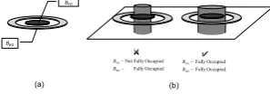
By considering the HMT in terms of SE occupancy, the traditional implementation of the HMT (which requires two erosions) may be simplified by combining BFG and BBG into
a unified, composite, SE (B, shown in Fig.2a). The composite SE, B, is translated to each point x in the image,
( ) {
Bx= b+x b| ∈B}
. A point x∈Eis marked in the result ifthere exists a level,t∈T, which for all of the elements,
( )
FG FG x
b ∈ B , t≤I b( )FG , while, simultaneously, for all of the
elements,
(
)
BG BG x
b ∈ B , t>I b( )BG , i.e.
( ) ( ) 2 -1 if , | ( ) and | ( ) 0 otherwise
n
FG FG FG BG BG BG
B
t T b B t I x b b B t I x b
HMT I x= ∃ ∈ ∀ ∈ ≤ + ∀ ∈ > +
(15)
This technique is illustrated in Fig.2 where a combined, composite SE is shown in Fig.2(a) and an example of this SE discriminating between similar objects is shown in Fig.2(b).
Not Fully Occupied Fully Occupied
FG BG B B −
− Fully Occupied Fully Occupied
FG BG B B − −
BBG
BFG
(b) (a)
Fig.2 The HMT implemented using a composite SE. (a) The composite SE
where elements of BFG are shown in dark gray and elements of BBG shown
in light gray. (b) The SE searching for places where it is fully occupied in the image.
Our definition of the grayscale HMT allows this operator to be calculated in one pass of the image instead of the common two pass method followed by an intersection, summation or comparison of the two resultant images. As a
result, the transform is faster and simpler than the standard method.
C. The Hit-or-Miss-Transform in noise
Fundamentally, a “hit” i.e. an object which is detected and marked by the HMT, is one which satisfies the conditions stated in Section II.B. This strict definition of the HMT requires that the composite SE must be fully occupied in both the foreground and background of the image for successful detection of an image feature. Often, when features are distorted by noise or if image features contain a large amount of internal texture, it is not possible for B to be fully occupied in the image even if its geometry matches that of the feature. This causes the HMT to miss objects that should be detected as illustrated in Fig.3.
BBG
(a) (b) (c)
[image:4.595.365.499.267.305.2]BFG
Fig. 3 Operation of the HMT in noise (a) Composite SE that can be used to detect a circle (b) Fully occupied, composite SE detecting the object of interest (c) Composite SE cannot be fully occupied due to noise
Fig. 3(a) shows a composite SE which can be used to detect circular objects using the standard HMT. BFG is a
solid disk and BBG is a solid ring. The black line in Fig.3(b)
represents a noise free shape which is to be detected using the SE shown in Fig.3(a). In this case, the elements of B
corresponding to BFG are fully occupied by the shape and
the elements corresponding to BBG are simultaneously fully
occupied by its background at all levels t, until t is greater than the intensity of the shape. This feature and any feature that has not been corrupted by noise and whose dimensions are greater than BFG and less than that of BBG will be
detected by the HMT when using this SE.
In the case that an object of interest, its edges, or both are corrupted by noise, the elements of B corresponding to
BFG and BBGmay never be simultaneously fully occupied by
the object. This is illustrated in Fig.3(c) where both the foreground and background regions of the object shown in Fig.3(b) have been perturbed by noise. Since some of the foreground pixels within the object are at a level t that is lower than the level of its noisy background, there is no level t at which BFG and BBG can be simultaneously fully
occupied. As a result, the HMT will fail to recognize this feature as an object of interest. For the same reasons stated here, objects which have internal texture, such as biological cells, may fail to be detected by the standard HMT.
III. APERCENTAGE OCCUPANCY HIT-OR-MISS
-TRANSFORM
In the standard HMT the foreground structuring element,
BFG, must fit entirely within the foreground of the object
and the background SE, BBG, must fit entirely within the
[image:4.595.88.237.600.652.2]otherwise legitimate hit occurring.
The idea behind the POHMT is to make the detection process less sensitive to moderate amounts of noise (or texture) in the image. We propose relaxing the constraint that the SEs must be 100% occupied and allow them to be only partially occupied and to still record a ‘hit’. Attempts at relaxing these strict constraints have been proposed in [7], [14], [19] and [20], however, in this paper we introduce a new design tool in order to set the appropriate level of partial (or percentage) occupancy. This tool may also be used in order to set the parameters for equivalent methods in an objective rather than an empirical way.
This paper builds upon a Percentage Occupancy Hit or Miss Transform (POHMT) introduced in [18], which allows a percentage of the SE to be “punctured” by noise or texture in a signal and still detect a “hit”. This section first defines a method that can be used to calculate the extent to which BFG
and BBG are occupied by a signal for all levels t∈T when
their origin is coincident with any pointx∈E. The POHMT is then defined using this approach, to allow objects to be detected in places where the SE is only partially occupied by the signal.
A. Calculating the occupancy of Structuring Elements
We have shown that a grayscale HMT, using flat SEs, can be implemented with a single, composite SE, which searches the image to identify places where its foreground and background elements are simultaneously 100% occupied. By designing the SE to match the geometry of an object in both the foreground and background and measuring the extent to which the object occupies the SE when coincident with an image feature, we can estimate how far we must relax the 100% occupancy requirement in order to detect this object in the presence of noise.
To facilitate this explanation and its comprehension, we first consider BFG and BBG separately before showing how
the two can be combined (as in Section II.B) into a single operator, capable of processing an image in one pass. Separating the two SEs and measuring the extent to which features occupy BFG and BBG allows us to plot this data to
determine a minimum occupancy requirement so that the SEs can detect objects in the presence of noise or texture.
The number of elements of BFG that are occupied by a
signal in the foreground can be calculated by translating BFG
to a point x in the image, and∀ ∈t T , calculating the
cardinality (Card) of the set, ( )
{
( )}
, |
FG x t FG FG FG
B = b ∈B I x b+ ≥t ,
of image pixels which are coincident with BFG and have
intensity greater than or equal to t. For all t∈T, we calculate the foreground occupancy,
,
x t FG
O ,
{
(
)
}
, , .
x t
FG FG x t
O =Card B (16)
By an equivalent technique, it is possible to measure the extent to which a feature occupies the background SE, BBG,
(
)
{
}
, , .
x t
BG BG x t
O =Card B (17)
In this case, BBG is translated to a point
x
∈
E
and ∀ ∈t T ,we calculate the background occupancy, ,
x t BG
O , i.e. the
cardinality of the set, ( )
{
( )}
, |
BG x t BG BG BG
B = b ∈B I x b+ <t , of
image pixels, coincident with BBG, that have intensity less
than t.
Using (16) and (17), we obtain two, one dimensional arrays,
,
x t FG
O and
,
x t
BG
O , of length 2n which contain the
number of elements that are occupied by the signal in BFG
and BBG respectively at each level t. The elements of both
arrays can be converted to percentages such that we obtain the percentage occupancy of BFG and BBG for all t∈T
when their origin is coincident with a point
x
∈
E
. We denote the percentage occupancy of the foreground andbackground SEs, POFG and POBG respectively
where,∀ ∈t T ,
(, )
, 100
x t x t
FG FG
FG
O PO
Card B
= × (18)
(, )
, 100.
x t x t
BG BG
BG
O PO
Card B
= × (19)
Since the cardinality of BFG and BBG is generally known,
POFG and POBG may be calculated directly, ∀ ∈t T, using,
( )
{ }
( )
,
|
100
x t
FG FG FG
FG
FG
Card b B I x b t PO
Card B
∈ + ≥
= ×
(20)
( )
{ }
( )
,
|
100
x t
BG BG BG
BG
BG
Card b B I x b t PO
Card B
∈ + <
= ×
(21)
The advantage of working in a relative measure such as percentages is that when calculating the POHMT, being able to specify a minimum percentage of the SE that must be occupied for successful detection rather than the actual number of SE elements makes the transform more general. Calculating POFG and POBG also allows these quantities to
be plotted against each other in the form of a percentage occupancy (PO) plot such as those shown in Fig.4.
Fig.4(a) shows a noise free, synthetic, 8 bit grayscale image, containing a homogeneous circle on a uniform, dark background. By designing BFG such that it can be contained
entirely within this circle and the elements of BBG to form a
ring to encompass the disk, POFG and POBG may be
calculated using (20) and (21). We have plotted POFG and
POBG against intensity for the noise free feature in Fig.4(b)
to illustrate how these quantities vary with t. By observation of Fig.4(b), it is clear that BFG is 100% occupied until t =
150 i.e. until BFG is above the signal and BFG is 0%
occupied for t >150. We can also see that BBG is 0%
each level t. By interpolating these discrete points we obtain a profile, which, in this case, takes the form of a right angle.
0 50 100 150 200 250
0 20 40 60 80 100
Extent to which BFG and BBG are occupied
Intensity
P
O
o
f
S
E
s
POFG
POBG
(b)
(a) (c)
(e) (d)
(f)
Critical Point
Critical Point T=50
T=150
0 20 40 60 80 100
0 20 40 60 80 100
PO Plot
PO
FG
P
OBG
0 50 100 150 200 250
0 20 40 60 80 100
Extent to which BFG and BBG are occupied
Intensity
P
O
o
f
S
E
s
POFG
POBG
0 20 40 60 80 100
0 20 40 60 80 100
PO Plot
PO
FG
P
[image:6.595.345.512.119.199.2]OBG
Fig. 4 Images and their PO plot (a) Synthetic image (b) Plot of POFG and
POBG against intensity (t) for (a). (c) PO plot indicating that the standard
HMT will detect the noise free object. (d) Noisy cell image (e) Plot of
POFG and POBG against intensity (t) for (d). (f) PO plot indicating the
HMT will not detect the cell. N.B. If the HMT will not be affected by noise ((a), (b) and (c)), the critical point may be a set of points, the cardinality of which gives the number of times that the SEs fit the feature.
The image shown in Fig.4(a) is not perturbed by noise and the feature of interest does not exhibit internal texture, hence the standard HMT, using the SEs described could be used to detect this object. This is reflected in the PO plot since it shows that there is at least one level, t, such that when BFG and BBG are centered at
x
∈
E
, BFG and BBG aresimultaneously, 100% occupied. This is indicated in Fig 4(c) by the line forming a right angle which intersects the point on the 45° diagonal where, POFG = POBG = 100.
However, if the image is corrupted by noise, the PO plot will not form the ideal right angle but will instead tend towards a curve. This is demonstrated using the image of a noisy cell shown in Fig.4(d). Again, we have plotted POFG
and POBG against intensity in Fig.4(e), and the
corresponding PO plot, generated by plotting POFGvs POBG
and interpolating, is shown in Fig.4(f). In this case, by examining Fig.4(e), it is clear that there is no level t for which POFG = POBG = 100% and hence the HMT will fail to
detect this feature using the SEs described. This is reflected in the PO plot shown in Fig.4(f) since instead of forming the right angled profile shown for the noise free shape, the PO plot in the case of noise, tends towards a curve which crosses the 45° line where (POFG = POBG) < 100. It should
be noted that the critical point on the PO profile (Fig.4(c) and Fig.4(f)) is the point where the curve crosses the 45° line. This point is equivalent to the point at which POFG and
POBG intersect in Fig.4(b) and Fig.4(e). The critical points
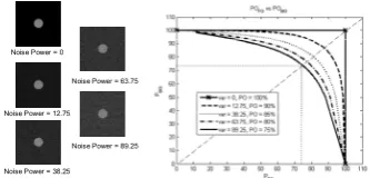
and their equivalences in the plots are highlighted in Fig.4. As the noise and texture is increased, the distance between the curve and this ideal right angle increases. This effect is demonstrated in Fig.5 where zero mean, Additive White Gaussian Noise (AWGN) of increasing power has been added to a synthetic image similar to the one shown in Fig. 4(a).
The PO plot shown in Fig.5 can be used to set a minimum percentage occupancy requirement for B such that the circle may be detected, using this SE, even in very noisy conditions. Since there is only one object (the grey circle) in each image on the left of Fig.5, the minimum occupancy
requirement can be set for the image with the highest noise power.
Noise Power = 12.75
Noise Power = 38.25 Noise Power = 0
Noise Power = 63.75
Noise Power = 89.25
Fig.5 The effect of noise on the PO plot. (left) Images corrupted by AWGN of zero mean and increasing power. (right) Corresponding PO plots for the object in each image with increasing noise power.
That is, by reference of the PO plot in Fig.5, setting the minimum occupancy requirement of B to 75% guarantees that the gray circle will be detected by the POHMT in all five images. This is clear from the PO plot which indicates that 75% is the lowest occupancy of the SE in all of the images. If there were other objects in the image, setting the minimum PO requirement so low, may invoke erroneous hits in the images that are distorted by noise of lower power. Increasing the minimum PO appropriately, using the PO plot as noise power decreases, will reduce the likelihood of erroneous detection.
It is possible for BFG and BBG to be combined to form a
composite SE, B, as in Section II.B. This allows the extent to which the elements of B corresponding to the foreground,
FG
b ∈B, and background, bBG∈B, of an image to be calculated simultaneously for allt∈T, in a single pass. The highest percentage of B, denoted POB that is occupied
by a signal for all t∈T, when its origin is coincident with a point x∈E may be calculated by finding the critical point that was introduced in Fig.4. In the PO plot, the critical point is the one that crosses the 45°line which occurs when
POFG =POBG. However, the values on the curve are discrete
points at finite integer values of t and hence it is unlikely that a data point belonging to this profile would lie exactly on the 45°diagonal. We must therefore find the point in the PO plot which is closest to the one that intersects the line to determine the value of this critical point. Given that the critical points shown in Fig.4(b) and Fig.4(e) are equivalent to those shown in Fig4.(c) and Fig.4(f) respectively, it can be seen that the critical point may be most conveniently computed using,
{
}
, ,
( ) max min , .
x t x t
B FG BG
t T
PO x PO PO
∈
= (22)
In (22), the quantities POFG and POBG may be calculated
x E
∀ ∈ using (20) and (21). The POHMT, which is introduced in the next section, uses POB to determine
whether or not a pixel at position x∈Eshould be marked, as a hit, in the output of this transform, based on the extent to which POB is occupied at each position in the image.
B. The POHMT
[image:6.595.98.236.119.227.2]noisy images by allowing objects that occupy only a percentage of the SE to be marked in the output of this transform. The POHMT can be calculated ∀ ∈x E,
[ ]
2 -1 if ( )
( ) ,
0 otherwise
FG BG n
B B B B
PO x P
POHMT∈ x
≥
=
∪
(23)
where POB is calculated using (22) and P is the minimum
percentage of the SE that must be occupied for successful detection of an image feature. The value of P can be set by trial and error, or, if the power and distribution of noise that corrupts a signal is known, then an accurate value for P may be calculated using noise models. A third technique, which we propose in this paper, is to measure an appropriate value for P using the PO plot and a set of test images that is representative of the real data. By designing SEs to best match the geometry of image features that are to be detected, the method described in the previous section can be used to generate a PO plot for each object of interest in the set. The PO plot for each object can then be used to find a minimum value for P such that all features of interest will be detected in all images using the POHMT. This can be done by observation of the PO plot, or, alternatively, P can be determined automatically by calculating the critical point using (22). An example of generating a PO plot, using it to set P and the result of applying the POHMT to a noisy image containing cancer cells is shown in Fig.6, where the images are inverted for convenience when printing.
(b)
(a) (d)
0 20 40 60 80 100
0 20 40 60 80 100
PO Plot
POFG
P
OB
G
Top Left Cell Top Right Cell Bottom Left Cell Bottom Right Cell
(c)
Fig.6 Example of POHMT using a PO plot to set P. (a) Original, noisy image. (b) PO plot showing the PO profile for each cell using the same composite SE. (c) Binary marker produced by the POHMT (d) Result of applying the POHMT and performing an opening by reconstruction.
By observation of Fig.6(a), it is clear that there are four cells in the image. Each cell has different characteristics in terms of shape, intensity and noise. To detect these cells using the POHMT, the geometry of B was set using a priori knowledge of the shapes and sizes of the cells. The elements of B used to probe the foreground of the image were designed as a flat disk measuring 90 pixels in diameter such that it could fit inside that smallest cell in the image (bottom left cell in Fig.6(a)). The elements of B used to probe the background of the image formed a ring with an inner diameter of 110 pixels which was designed to encompass the largest cell (bottom right of Fig.6(a)). The extent to which the cells occupied B was measured by centering B on each cell and in turn and using (20) and (21) to calculate
POFG and POBG and generate the PO plot for each cell as
shown in Fig.6(b). By interpretation of the plot, it is clear that setting P to any value less than or equal to 70% is sufficient to ensure that all four cells will be detected by the
POHMT using B.
The POHMT was calculated ∀ ∈x Ewith P set to 70%. The POHMT produced a binary marker, as shown in Fig.6(c) which contains four groups of marker pixels in the same locations as each of the four cells in the Fig.6(a). Performing an opening by reconstruction using the original image as the “mask” and the result of the POHMT as the “marker” produced the image shown in Fig.6(d). It should be noted that the standard HMT did not detect any of the cells as predicted by the PO plot. We also point out here, that the POHMT is an extension of the HMT and hence the standard HMT can be implemented as a special case of the POHMT. Setting P to 100% in (23) and calculating the POHMT of an image will give the same result as any of the grayscale HMTs discussed in Section II of this paper.
IV. EXTENSIONS OF THE HMT AND THE PO PLOT
We have demonstrated that the PO plot can be used as a design tool to set the only parameter P for the POHMT. In addition to this, we show here that the PO plot may be used as a tool by other researchers to set corresponding parameters for their own routines. Further, we show that by exploiting the information contained within the PO plot, it is possible to discriminate between image features, having similar properties, using a single composite SE.
A. A design tool for existing grayscale HMTs in noise
In addition to the grayscale extensions of the HMT that have been presented by various researchers (as discussed in Section II of this paper), numerous methods have been proposed which aim to generalize the HMT to make it more robust to noise. We review here a few of these techniques and provide a method which exploits the properties of the PO plot in order to set parameters for these methods.
In [14], the authors present a “Generic solution to improve noise robustness” where they indicate that the grayscale HMTs proposed by Ronse and Soille can be made more robust to noise if the distance between the two SEs,
BFG and BBG, is increased. In [14], an example of how to
modify this distance is given as, ' and '
FG FG BG BG
B =B −l B =B ,
or, ' '
and
FG FG BG BG
B =B B =B +l. However, no formula or method is provided that can be used to calculate an appropriate value for l.
It is possible to use the PO plot to determine an appropriate value for this parameter, l, by forcing the PO plot to form the ideal right angle. By calculating a distance,
d, from the PO arrays, and shifting the elements of either
POFG or POBG, by this distance, we can force the PO plot to
form a right angle despite any noise or texture in the image. We calculate d, as the difference between the highest level,
t, for which BFG is 100% occupied and the lowest level, t,
for which BBG is 100% occupied. More formally,
(
)
(
)
, ,
max | FGx t 100 min | BGx t 100 .
t T t T
d t PO t PO
∈ ∈
= = − = (24)
the right or left respectively, to obtain either PO’FG or
PO’BG. By plotting PO’FG vs. POBG or POFG vs. PO’BG, we
obtain the right angled plot which implies that by setting l = d, we can accurately set the distance between SEs using the method described in [14] to improve the noise robustness of the RHMT or the UHMT. That is, the level d that is calculated in order to force the plot to form the right angle, is equivalent to the minimum distance that must be allowed between BFG and BBG such that the feature of interest may be
detected by either of these HMTs in the presence of noise. To demonstrate this technique we use the synthetic image shown in Fig.7(a) which has been corrupted by zero mean, AWGN, of variance 9.22.
0 20 40 60 80 100
0 20 40 60 80 100
PO Plot
POFG
P
OBG
d = 4 d = 8 d = 12 d = 16 d = 20
Increasing d
0 20 40 60 80 100
0 20 40 60 80 100
PO Plot
POFG
P
OB
G
(e)
(a) (c)
(d) (b)
0 100 200 300 400 500
100 105 110 115 120 125 130
Column Index
G
ra
yle
ve
l In
te
n
sit
y
Fig.7 Setting the SE separation for Ronse’s and Soille’s HMTs. (a) Noisy synthetic image. (b) Histogram equalization of (a) for visualization of noise. (c) Intensity profile of image center row, no noise (blue), noise corrupted signal (green). (d) PO plot obtained before (green) and after
(blue) shifting the elements of POFG by d as well as intermediate plots for
increasing d. (e) PO Plots obtained before (green) and after (blue) setting
the SE separation to d and calculating POFG and POBG.
For the purpose of illustrating the effect that the noise has on this signal, we have shown, in Fig.7(b), the image after histogram equalization, and in Fig.7(c), we show a 1D intensity profile taken from the center row of the image before and after the noise has been added. By generating the PO plot for the case where the distance between the SEs is initially zero, we can use (24) to calculate the distance d
that should be set between the SEs to allow this feature to be detected. By shifting the elements of POFG to the right by
d and plotting PO’FG vs POBG, we obtain the right angle as
shown in Fig.7(d). To demonstrate the way in which the plot is forced to form the right angle, we have shown three additional curves in the PO plot in Fig.7(d). These curves have been generated purely for example by setting d to values that lie between zero and the critical distance of 20 graylevels that was calculated using (24).
By reference of Fig.7(d), it is clear that as d increases, the plot gradually approaches the desired right angle before attaining this profile when d = 20. If the distance, d, between the SEs is sufficient to allow the HMTs defined by Ronse or Soille to detect the noisy feature, the PO plot that is generated after fixing this distance between the SEs and recalculating POFG and POBG, also forms the right angle.
This case is shown in Fig.7(e) where the distance between the SEs was set to 20 graylevels before calculating POFG
and POBG.
A drawback with the method in [14] of increasing the distance between the SEs is that it is prone to erroneous detections since any group of pixels lying between the SEs will be marked as a “hit”. When applying the RHMT or the UHMT and setting the distance between the SEs to be d as described, the disk in the noisy image is successfully detected. There are however, as expected, many erroneous “hits” in the resultant image. The POHMT on the other hand marks only the feature of interest.
The authors [14] also discuss the performance of the HMTs proposed by Barrat et al. and Khosravi and Schaefer when images are corrupted by noise. They conclude that since these HMTs already evaluate a distance between the SEs, the problem of finding a suitable distance is transformed into a problem of thresholding the result of their HMTs. It is possible to use the PO plot in the same fashion as before to determine this threshold, where the threshold is equivalent and can therefore be equated to the distance d that was previously calculated using (24).
By performing the grayscale HMTs proposed by Barrat and Khosravi and thresholding the results at d=20, we successfully detect the disk in the center of the image. However, as is the case with the previous example, a large number of erroneous detections appear in the result when using this technique. Thresholding the result of these HMTs at a level less than d does not allow successful detection of the circle in noise, however, the result still contains a high number of false positives. The same is true for the RHMT and the UHMT, where setting the distance between the SEs to be less than 20 graylevels results in erroneous “hits” while the feature of interest is not detected.
In [14], the authors state that if an image is corrupted by AWGN, and the variance of this noise is known, then the distance between BFG and BBG can be set to equal twice that
of the standard deviation of the noise. This theory can be verified by setting this distance between the SEs and generating a PO plot to form the ideal right angle as has been done in previous examples. This method is reliable if the power and distribution of the noise is known. Usually, this is not the case and hence the PO plot could be used in such situations, to calculate this parameter.
We have shown here, that the problem of defining a suitable distance between the SEs and finding a suitable threshold to apply to the result of the HMTs are equivalent as stated in [14]. We also show that these parameters can be estimated using the PO plot by finding the minimum distance, d, which forces the result to form the right angle. However, an issue with relaxing the conditions of the HMT using these techniques is that the transform becomes more susceptible to producing erroneous hits in the output image.
scale lengths, orientations and elongations. A measure of fitness is obtained for all patterns in the set of SEs at each point in the image, and a record of the best fitting SE at each pixel is stored as well as a measure of how well this SE fits the image. This data is used to form a so called “Scoremap” which is thresholded at a particular level to produce a binary marker image from which detected features can be reconstructed.
For the FHMT, the PO plot could be used to set the ideal distance between the SEs, or to provide an indication of a suitable threshold that can be used on the output of this transform. Additionally, the PO plot and a suitable set of training data could be used to set a minimum occupancy requirement for a single SE, or at least a small subset taken from the large set of SEs that are used currently. This would allow the algorithm to execute, in the same way as the POHMT, in a fraction of the time taken by the current routine (2 minutes per image) described in [14].
B. A discriminatory filter
Often, features that are to be detected in an image are not geometrically identical. If, therefore, we wish to extract from an image, a number of features, which differ from each other in terms of shape and size, we can design a number of composite SEs i.e. one to match the geometry of each object that we seek in the image. We can then perform a grayscale HMT using each of the composite SEs in turn before calculating the union of all the resulting binary images to obtain a single image that contains markers for each image feature that has been detected. That is of course assuming that the HMT will not fail to detect these features due to noise or texture in the image.
As was illustrated in Fig.6, the POHMT allows multiple objects which are geometrically very different to be detected using just one composite SE in a single pass of the image. This can be achieved by exploiting the information contained within the PO plot in order to determine an appropriate level for P such that we can guarantee to detect all the features in this image. The PO plot does however provide a further advantage in that we may set P in such a way that we can discriminate between image features using just one composite SE. The simplest case of discriminating between features using the POHMT is to set the value of P
high enough to eliminate objects which simultaneously occupy a maximum percentage of B that is always less than
P. An example of selectively detecting cells in the image by varying P using the information contained in the PO plot is shown in Fig.8.
Clearly, by reference of Fig.8(a), setting the level of P to any value that lies between the curve representing the cell in the bottom right and left of the image, we can eliminate the cell in the bottom left while successfully detecting the other three cells. In Fig.8(c) we have extracted only three of the four cells shown in Fig.8(b) by setting P=75% in order to eliminate the cell in the bottom left of the image for which the maximum, simultaneous occupancy of the SE when coincident with this cell is 70%. By raising the level of P to 90% and then 96% in accordance with the PO plot shown in
Fig.8(a), we can extract respectively two cells (Fig.8(d)) then one cell (Fig.8(e)). Evidently, the PO plot is an extremely powerful design tool, as it provides information that allows objects to be detected selectively using one composite SE in a single pass of the image.
0 20 40 60 80 100
0 20 40 60 80 100
PO Plot
POFG
P
OB
G
Top Left Cell Top Right Cell Bottom Left Cell Bottom Right Cell
(a)
(c)
(d) (e)
P=75%
3 cells
P = 96% 1 cell P = 90%
2 cells
(b)
Fig.8 Example of POHMT operating as a discriminatory filter. (a) PO plot for the four cells in (b). (b) Noisy image containing four cells. (c) Three of
the four cells detected by setting P =75%. (d) Two of the cells detected by
setting P =90%. (e) One of the cells detected by setting P = 96%.
The case demonstrated here is a powerful yet trivial one since it is obvious that increasing the level P or in other words increasing the strictness of the transform results in objects being discarded in the detection process.
What is more interesting, is that by a similar technique to the one described above, it is possible to isolate any of the four cells in the image shown in Fig.8(b) and hence we can segment any combination of the image features using just one composite SE. In this case, the PO plot can be used as a shape descriptor which allows us to use one composite SE to discriminate between objects of interest in an image and objects which may have very similar geometrical properties in the spatial domain, for example, the two cells at the top of the image. Fig.9 shows each of the cells being extracted on their own using the same composite SE and the POHMT.
(b)
(a) (c) (d) (e)
Fig.9 POHMT operating as a discriminatory filter (a) Image containing four cells of different shape and size. (b) Bottom left cell isolated. (c) Top right cell isolated. (d) Bottom right cell isolated. (e) Top left cell isolated.
The results shown in Fig.9 can be easily achieved by firstly detecting and reconstructing all of the four cells in the image. Then, by detecting the objects that are not desired and reconstructing this image, the difference image can be calculated such that only the features specified by a user etc. are picked out by the POHMT.
V. EXPERIMENTAL RESULTS
those used to optimize median filtering [21] and morphological operators [22]. However, instead of searching for the min, median or max value in the window, the POHMT searches for the rank specified by P.
An example of the noisy biological images (of an immune system cell) is shown in Fig. 10 where we have chosen three of the images (Fig.10(a)) to be used as a training set in order that P can be determined and used to detect the features of interest in our test set (Fig.10(b)). We can see a small group of pixels in each image in Fig.10 that represents the feature of interest, while the rest of the image contains noise and other features that are not of interest. The images are extremely noisy, and, by observation of the data, it is evident that the shape and orientation of the cell changes between the images.
(a)
(b) (c)
Fig. 10 The image set containing the cell of interest and some other features where the entire image is submersed in noise. (a) Training set to
determine an appropriate value for P. (b) The set of test images in which
we seek the feature after P has been fixed using the PO plot for the test
set.(c) PO plot obtained for the training set shown in (a).
The first stage in the process is to generate a PO plot for each feature of interest in the test set in order to determine an appropriate level for P. Although the cell is not a constant shape and size in all images, we can design B such that its elements corresponding to BFG will fit inside it in
each image. Similarly, BBG was designed to encompass all of
the features of interest in each image to guarantee that we can detect the cell in all possible orientations and variations of shape and size. By increasing the spatial distance between the SEs, as we are here, it can be argued that the transform may produce erroneous hits. If a problem occurs, this issue can easily be overcome by exploiting the discriminatory property of the POHMT shown in Section IV B. We also note that although automatic techniques are available for SE design, we have used a manual method here to compare our method with the one presented in [14]. We have used square SEs for processing simplicity, however, this may be readily extended to arbitrarily shaped SEs using the method described in [22]. B was used to generate a PO plot for each image in the training set in order to obtain a suitable level for P, such that the feature could be detected in the test set, without picking up erroneous hits. The PO plot, generated for the training set, is shown in Fig. 10(c). Clearly, by reference of the PO plot, setting P=81% is sufficient to ensure that this feature may be detected using one composite SE for the entire test set. The POHMT was calculated for each image in the test set where the results of applying this transform and reconstructing the features of interest that have been marked
are shown in Fig.11.
We also calculated the average processing time using the described SEs when analyzing this image on a PC with a Pentium IV processor. The image is 512 x 512 pixels in size and the average time taken to process an image was measured to be 0.87s. This does not include the opening by reconstruction which is performed largely for illustration and is not normally required in a practical detection or feature recognition system. To improve visibility in Fig.11, we have dilated the each image resulting from the opening by reconstruction.
(b)
(a) (c) (d) (e)
Fig.11 Result of applying opening by reconstruction to the result of the POHMT for each image in Fig.10(b).
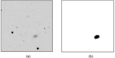
We have also tested our routine on the images used in [14] to compare the performance and efficiency with the one described by Perret et al. We show an example of the POHMT detecting an LSB galaxy in Fig.12 where the contrast of the image shown in Fig.12(a) has been enhanced to make the LSB clearly visible. The average processing time of our routine was 4 seconds per 512 x 512 image which is a substantial improvement compared to the 2 minute execution time of the optimized routine presented in [14].
For the example shown, our method is faster and simpler to implement than the method proposed by Perret et al [14] since it only requires one composite SE. Further, we point out here that we do not optimize our routine by sub-sampling the image, the SE, or by using any potentially lossy, heuristic techniques.
(b) (a)
Fig.12 The POHMT detecting a LSB galaxy. (a) Original noisy image containing a LSB galaxy in the lower right quadrant of the image. (b) The output of the POHMT when processing the image in (a).
[image:10.595.316.550.224.276.2] [image:10.595.45.283.275.354.2] [image:10.595.332.534.508.611.2]