City, University of London Institutional Repository
Citation
:
Lorenzoli, D. and Spanoudakis, G. (2009). Detection of Security and
Dependability Threats: A Belief Based Reasoning Approach. In: Falk, R., Goudalo, W., Chen,
E. Y., Savola, R. and Popescu, M. (Eds.), Emerging Security Information, Systems and
Technologies, 2009. SECURWARE '09. Third International Conference on. (pp. 312-320).
IEEE.
This is the unspecified version of the paper.
This version of the publication may differ from the final published
version.
Permanent repository link:
http://openaccess.city.ac.uk/626/
Link to published version
:
http://dx.doi.org/10.1109/SECURWARE.2009.55
Copyright and reuse:
City Research Online aims to make research
outputs of City, University of London available to a wider audience.
Copyright and Moral Rights remain with the author(s) and/or copyright
holders. URLs from City Research Online may be freely distributed and
linked to.
City Research Online:
http://openaccess.city.ac.uk/
[email protected]
Detection of Security and Dependability Threats: A Belief Based Reasoning
Approach
Davide Lorenzoli, George Spanoudakis
Department of Computing, City University London
E-mail: [email protected], [email protected]
Abstract
Monitoring the preservation of security and dependability (S&D) properties during the operation of systems at runtime is an important verification measure that can increase system resilience. However it does not always provide sufficient scope for taking control actions against violations as it only detects problems after they occur. In this paper, we describe a proactive monitoring approach that detects potential violations of S&D properties, called “threats”, and discuss the results of an initial evaluation of it.
I. INTRODUCTION
Monitoring security and dependability (S&D) properties during the operation of software systems is widely accepted as a measure of runtime verification that can increase system resilience to dependability failures and security attacks. Runtime monitoring of S&D properties is particularly important for systems that deploy distributed components running and communicating over heterogeneous infrastructures and networks dynamically (e.g., web service based, mobile and/or ambient intelligence systems). This is because, as the operational conditions of these systems change, the S&D mechanisms used by the systems and their components may become ineffective and, when this happens, the systems need to adapt or replace the deployed S&D mechanisms to ensure the preservation of the desired S&D properties.
To address the monitoring needs of such systems, we have developed a monitoring framework, called
EVEREST (EVEnt RESoning Toolkit). EVEREST
supports the monitoring of different types of S&D properties (e.g., confidentiality, availability and
integrity) that are expressed as rules in an Event
Calculus [10] based language called EC-Assertion
[4][8]. The rules expressing such properties are checked against streams of runtime events that EVEREST receives from event captors associated with the different components of the monitored system.
EVEREST has been developed as part of the runtime platform of the EU F7 project SERENITY project and to enable monitoring with distributed events, it supports the synchronisation of the clocks of event captors and optimised event management. When it detects a violation of an S&D property, EVEREST reports the violation to the runtime platform of SERENITY which has responsibility for taking control action (e.g., deactivate or replace the system components that have caused the violation).
Whilst the core monitoring capabilities of EVEREST are effective for detecting violations of S&D properties once they have occurred, post-mortem detection does not always provide sufficient scope for taking control actions that could contain or repair a violation. To address this shortcoming, we have extended EVEREST with mechanisms that enable it to detect potential violations of S&D properties, called
S&D threats, and measure how likely is for them to occur. An S&D threat report can be used by the runtime platform for triggering automatic preventive actions for violations (e.g., deactivate the component that causes
the problem or block any further interactions with it).
To detect S&D threats, EVEREST determines patterns of runtime events that would violate different monitoring rules and uses them to monitor the threat likelihood of different rules. More specifically, as runtime events arrive they are matched with rules and if a match is found the events are used to partially instantiate the rules. Then, for each partially instantiated rule, EVEREST computes a belief indicating how likely it is for the missing events of the rule to occur. These beliefs are computed based on functions founded in the Dempster-Shafer (DS) theory of evidence [12]. The reason for adopting the DS theory is due to uncertainty regarding the genuineness of the runtime events
received by EVEREST − an event may, for example, be
availability of evidence confirming the plausibility of these explanations.
In the rest of this paper, we present our approach for S&D threat detection and give the results of an initial experimental evaluation of it. More specifically, Section II presents an overview of EVEREST; Section III outlines threat detection using an example; Section IV presents the functions used to estimate threat beliefs; Section V presents belief graphs which are used to combine belief functions; Section VI presents an initial evaluation of our approach; Section VII presents related work; and, finally, Section VIII provides conclusions and outlines directions for future work.
II. EVEREST:AN OVERVIEW
A detailed description of the core monitoring capabilities of EVEREST is beyond the scope of this paper and may be found in [4]. It is however important to explain how the threat detection mechanisms that we describe in this paper are connected to other components of the toolkit. Thus, in the following we provide an overview of EVEREST and discuss threat detection in its context.
As shown in Figure 1, EVEREST has five main
functional components, namely an Event Collector, a
Monitor, a Diagnosis Tool (DT), a Threat Detection
[image:3.595.69.284.402.578.2]Tool (TDT), and a Manager.
Figure 1. The architecture of EVEREST
The event collector provides the API for the notification of events that are captured by event captors associated with the system that is being monitored and its components, and notifies these events to the Monitor and TDT.
The Monitor checks if the received runtime events violate monitoring rules that specify the S&D properties of interest. This component has been implemented as an
Event Calculus reasoning engine and detects only violations that have definitively occurred without attempting to diagnose whether the events that have caused these violations are genuine. The latter analysis
is the responsibility of the diagnosis tool (DT). DT assesses the genuineness of runtime events and computes a belief measure for them. These belief measures are stored in an event database and become accessible to the threat detection tool.
The threat detection tool (TDT) receives the same stream of runtime events as the monitor but, instead of checking for definite violations of S&D rules, it checks for potential violations and computes belief measures indicating the likelihood of such violations.
The Monitor and TDT operate in parallel and store
their results in a violations database. This database is
accessed by the Manager which retrieves definite
violations and/or threat signals for potential violations and reports them to external components (e.g. the system that is being monitored) in a pull or push mode (push notifications of monitoring results are generated when external components subscribe for these results).
III. S&DTHREATS:AN EXAMPLE
To comprehend the mechanisms for threat detection in the rest of the paper, consider the following example of a monitoring rule:
Rule-1:
∀ _U: User; _C1, _C2: Client; _C3: Server; t1, t2:Time
Happens(e(_e1,_C1,_C3,REQ,login(_U,_C1),_C1 ),t1,ℜ(t1,t1)) ∧
Happens(e(_e2,_C2,_C3,REQ,login(_U,_C2),_C2 ),t2,ℜ(t1,t2)) ∧ _C1 ≠_C2 ⇒ ∃ t3: Time
Happens(e(_e3,_C1,_C3,REQ,logout(_U,_C1), _C1),t3,ℜ(t1+1,t2+1))
Rule-1 is specified to monitor the logging activity of the users of a system that is accessible from different distributed client devices. The rule states that if a user
_U logs on the system from some client device _C1
(i.e., when the event e(_e1, _C1, _C3, REQ, login(_U,
_C1), _C1) happens) and later he/she logs on from
another device _C2 (i.e., when the event e(_e2, _C2,
_C3, REQ, login(_U, _C2), _C2) happens), by the time of the second login (t2), he/she must have logged out
from the first device (i.e., an event e(_e3, _C1, _C3,
REQ, logout(_U, _C1), _C1) must have occurred).
Monitoring Rule-1 can be used to prevent users
from logging on from different devices simultaneously and, therefore, reduces the scope for masquerading attacks. Simultaneous logging provides scope for such attacks since a user who is logged on from different devices simultaneously may leave one of them unattended. When this happens, however, some other
user may start using the unattended device with _U’s
credentials. Blocking logging attempts that violate
Rule-1 would prevent such cases. Furthermore,
monitoring Rule-1 could detect cases where some user
gets hold of the credentials of another user _U and tries
Threat Detection Tool Diagnosis Tool
Event Collector
EVEREST
Monitor
Event Captor (System) Event Captor (System Component)
Manager Control Component
Event DB Violation
DB
Event notification Event/Violation retrieval
Event write Diagnosis request
e
e
to use them to log on with the identity of _U at the
same time when _U is logged from a different device.
Rule-1 above is specified in the rule language of
EVEREST that is based Event Calculus [10]. In this
language, S&D properties are expressed as rules of the
form B⇒H. The meaning of such rules is that when
their head H is True their body B must be True as well.
Rules of this form are used to specify conditions about the patterns of events that should occur in a system and their effects onto the system and its environment state. The occurrence of an event in a rule is specified by the
predicate Happens(E,t1,ℜ(t1,t3)). This predicate
expresses that an event E of instantaneous duration
occurs at some time point t1 that is within the time
range (t2, t3]. An event E is specified by a term of the
form e(_id, _s, _r, [REQ|RES], _sig, _c) where _id is
the identifier of the event, _s is the identifier of the
component that has sent the event (event sender), _r is
the identifier of the component which the event was
sent to (event receiver), REQ(RES) are constants
indicating whether the event is a request (REQ) or a
response (RES) from the sender, _sig is the signature
of the event (e.g., the signature of an operation if the event represents an operation call or response as in
Rule 1), and _c is the identifier of the component from which the event was captured (i.e., typically the sender
or the receiver of the event)1.
The detection of threats w.r.t. specific monitoring rules at runtime is based on the computation of a belief in the potential occurrence of runtime events that would violate the rules. The pattern of events that can violate a rule is determined by negating the rule and
getting its violation signature (i.e., B∧¬H for a rule of
the form B⇒H). The belief in a potential rule violation
is computed from beliefs in the genuineness of the events that have already occurred and match the rule’s violation signature, and beliefs in the potential occurrence of events which appear in the signature but have not occurred yet.
In the case of Rule-1, the violation signature that is
produced by negating the rule is: ∀ _U: User; _C1, _C2: Client;
_C3: Server; t1, t2:Time
Happens(e(_e1,_C1,_C3,REQ,login(_U,_C1),_C1 ),t1,ℜ(t1,t1)) ∧
Happens(e(_e2,_C2,_C3,REQ,login(_U,_C2),_C2 ),t2,ℜ(t1,t2)) ∧ _C1 ≠_C2 ∧ ∀ t3: Time
¬Happens(e(_e3,_C1,_C3,REQ,logout(_U,_C1), _C1),t3,ℜ(t1+1,t2+1))
Thus, the detection of threats for this rule during monitoring would need to be assessed in the following cases:
1A full description of the rule language of EVEREST is given in [4].
(a)When a login event matching e(_e1,…) but no login
event matching e(_e2,…) have been received. In
this case, the threat for the rule would be a
combined measure of the belief that the event _e1
which has been matched with the rule is genuine,
the belief that an event _e2 matching the rule will
occur within the time range (t1, t2], and the belief
that no event matching the event _e3 will occur in
the range (t1, t2].
(b)When a login event matching e(_e2,…) but no login
event matching e(_e1,…) has been received. In this
case, the threat likelihood of the rule would be a
combined measure of the belief that the event _e2
which has already been matched with the rule is
genuine, the belief that an event of type e(_e1,…)
matching the rule has already occurred within the
time range (latestTime(captor(_e1)), t2]2 but not
received by EVEREST yet, and the belief that an
event matching e(_e3,…) will occur in the range
(latestTime(captor(_e1)), t2].
(c)When a login event matching e(_e1,…) and a login
event matching e(_e2,…) have been received by the
monitor. In this case, the threat likelihood the rule would be a combined measure of the beliefs that the e(_e1,…) and e(_e2,…) events are genuine and
the belief that no event of type e(_e3,…) matching
the rule will occur in the time range (t1, t2].
(d)When a login event matching e(_e1,…) and an
event matching e(_e2,…) have been received by the
monitor and an event E has been received from the
event captor that should have sent e(_e3,…) at
some time point t’ > t2 indicating that e(_e3,…)
will not arrive. The absence of e(_e3,…) could be
derived from E in this case using the principle of
negation as failure (NAF). More specifically, since
t’ > t2 TDT knows that it cannot receive any event
with a timestamp earlier than t’ from the same
captor and therefore earlier than t2 (the
communication channels between captors and EVEREST follow the TCP/IP protocol). Thus, in this case, the threat likelihood of the rule would be
a combined measure of the belief that the e(_e1,…)
and e(_e2,…) events that have been matched with
the rule and the event E which provides the basis
for deriving ¬ e(_e3,…) are genuine.
The functions that we use to measure the above beliefs are discussed in the following.
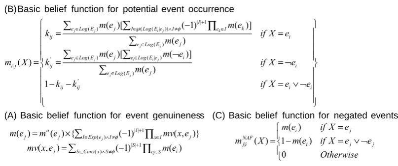
IV. BELIEF FUNCTIONS
The calculation of the overall belief in a potential rule threat requires the combination of basic beliefs of three types:
1. Basic beliefs in the genuineness of occurred events
(like _e1 and _e2 in case (c) above),
2. Basic beliefs in the occurrence of an event of a
specific type within a time range that is determined by another event (i.e., basic belief of seeing an
event like _e2 after an event _e1 has occurred as in
case (a) above), and
3. Basic beliefs in the validity of the derivation of the
negation of an event when another event’s occurrence indicates that the time range within which the former event should have occurred has
elapsed (i.e., basic belief in events like ¬e(_e3,…)
given another event E as in case (d) above).
A. Basic belief in event genuineness
The calculation of basic belief in the genuineness of events is based on the approach described in [11]. According to this approach, an event received by EVEREST is genuine if there is at least one valid explanation for it. The possible alternative explanations
of an event e are generated from assumptions about the
system that is being monitored. Assumptions are expressed as EC formulas having the same form as monitoring rules but are used for abductive and deductive reasoning without being checked as rules.
Given an event e that needs to be explained at time t,
the explanations generation process finds recursively all
the assumptions of the form Hn⇐ Bn, Hn-1⇐Bn-1, …,
H1⇐B1 where e matches with Hn and Bimatches with
Hi-1for all i=n…2. For all the different chains of such
formulas that may exist, B1is a possible explanation of
e. The belief in the validity of this explanation is then
computed by establishing all the runtime events (other
than e) that should have occurred as a consequence of
B1 if the latter was true and computing the basic belief
in at least of one of these events being genuine. The set
of the consequences of B1 is formally defined as:
Cons(B1) = {ec | {B1, Events(t − DW, t) |− ec and e≠ec))
where DW is parameter denoting the period of time of
interest in diagnosis, called diagnosis window.
Given the set of possible explanations EXP(e) of an
event e and the consequence set Cons(x) of each
element x of EXP(e), the basic belief in the genuineness
of e is computed by the function m(e) in Figure 2.
As discussed in [11], m (e) is defined as a DS basic
belief function (also known as mass or basic belief
assignment in the context of DS theory). The use of DS theory is because for some explanation consequences it might not be possible to establish with certainty whether they are confirmed by runtime events. This phenomenon arises in cases where the runtime event that would confirm an explanation consequence is
expected to occur at some time point t but as the
timestamp of the last event that was received from the
relevant captor (i.e., lastTime(captor(e))) is less than t,
it is impossible to establish with certainty whether the event has indeed occurred. Such cases arise due to
communication channel delays – an event E might have
occurred but not received by EVEREST yet when its occurrence needs to be established due to delays in the communication channel that transmits the event from the relevant event captor to the framework. Classic probabilities are unable to represent this uncertainty and, hence, we use DS beliefs.
B. Basic belief in potential event occurrences
The second type of basic belief functions that we use in threat detection measure the likelihood of the
potential occurrence or not of an event Ei, which has
not occurred yet, when another event Ej that Ei is
temporally constrained by has occurred. The likelihood of such conditional event occurrences is measured by
the basic belief function mi|j(X) in Figure 2. In the
definition of this function:
• Log(Ej) is a randomly selected sample of N events
of type Ej in the event log up to the time point when
mi|j is calculated. ⎪ ⎩ ⎪ ⎨ ⎧ ¬ ∨ = − = = − = − × = ⎪ ⎪ ⎪ ⎪ ⎭ ⎪ ⎪ ⎪ ⎪ ⎬ ⎫ ⎪ ⎪ ⎪ ⎪ ⎩ ⎪ ⎪ ⎪ ⎪ ⎨ ⎧ ¬ ∨ = − − ¬ = ¬ = = − = =
∑
∏
∑
∏
∑
∑
∑
∑
∑
∑
∏
≠ ∧ ⊆ + ∈ ≠ ∧ ∈ + ∈ ∈ ∈ ∈ ∈ ∈ ∈℘ ∧≠ + ∈ Otherwise e e X if e m e X if e m X m e m e x mv e x mv e m e m e e X if k k e X if e m e m e m k e X if e m e m e m k X m j j i j i NAF i j S x ConsS e S i
S j
I e Exp
I xI j
I j o j i i ij ij i E Log e j E Log
e j e LogEe i
ij i E Log e j E Log
e j I LogEe I I e I k
ij j i i j j j j
j i i j j j j
j i j k
[image:5.595.109.513.111.280.2]0 ) ( 1 ) ( ) ( ) ( ) 1 ( ) , ( )} , ( ) 1 ( { ) ( ) ( 1 ) ( ] ) ( )[ ( ) ( ] ) ( ) 1 ( )[ ( ) ( | ) ( 1 | | ) ( 1 | | ' ) ( ) ( ( | ) ' ) ( ) ( ( ( | )) 1 | | | φ φ φ events negated for function belief Basic (C) s genuinenes event for function belief Basic (A) occurrence event potential for function belief Basic (B)
• Log(Ei|e) is the set of the events of type Ei in the
event log that have occurred within the time period
determined by e and up to the time point when mi|j
is calculated
• I (I∈ ℘(Log(Ei|e))) is an element set in the
powerset of Log(Ei|ej)
• m(e) is the basic belief function defined in Part (A)
of Figure 2 in the case of non negated events Ej.
According to the above definition, mi|j(X) measures
the basic belief in the occurrence of a genuine event of
type Ei within the time range determined by events of
type Ej, as the average belief of seeing a genuine event
of type Ei within the time range determined by a
genuine event of type Ej. More specifically, for each
occurrence of an Ej event, mi|j(X) calculates the basic
belief of seeing at least one genuine event of type Ei
within the period determined by Ej. Assuming that the
set of such Ei events is Log(Ei|ej), this basic belief is
calculated by the following formula:
∑
I∈℘Log E e ∧I≠φ − +∏
e∈I k Ij
i| )) k m e
( (
1 |
| ( )
) 1 (
The above formula measures the basic belief in at
least one of the events in Log(Ei|ej) being a genuine
event, i.e., an event that has at least one explanation confirmed by other events in the log of the system, and uses the basic belief in the genuineness of individual
events m(Ei) for positive events. Thus, mi|j(X) discounts
occurrences of events of type Ei which are not
considered to be genuine, and the higher the number of
genuine events of type Ei within the period determined
by an Ej event, the larger the basic belief in the
occurrence of at least one genuine event of type Ei that
it generates. It should also be noted that mi|j(X) takes
into account the basic belief in the genuineness of each
occurrence of an event of type Ej within the relevant
period (i.e., mi(ej)) and uses it to discount the evidence
arising from Ej events which are not considered to be
genuine themselves.
C. Basic belief in negated events
The basic belief functions that we have introduced so far do not cover cases where the absence of an event is deduced by the NAF principle. As we discussed earlier, EVEREST uses this principle to deduce the
absence of an event E (i.e., ¬E) that is expected to
occur within a specific time range [tL, tU] when it
receives another event E’ from the event captor that
should sent E with a timestamp t’ that is greater than tU
(t’ > tU) and has not received E up to that point.
Considering, however, that the event E’ which triggers
the application of the NAF principle in such cases might not be a genuine event itself, it is necessary to
estimate a basic belief in the conjecture of ¬E. The
function that measures this basic belief is the function
mNAF
[image:6.595.311.532.116.297.2]j|i in Figure 2.
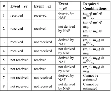
Table 1. Combinations of basic belief functions for Rule 1
# Event _e1 Event _e2 Event
¬_e3
Required Combinations
1 received received derived by NAF (m1⊕ m2) ⊕
mNAF 3|u
2 received received not derived by NAF
(m1⊕ m2) ⊕
m3|2
(m1⊕ m2) ⊕
m3|1
3 received not received derived by NAF (m1⊕ m2|1) ⊕
mNAF 3|u
4 received not received not derived by NAF (m1⊕ m2|1) ⊕
m3|1
5 not received received derived by
NAF (mmNAF2⊕ m1|2) ⊕ 3|u
6 not received received not derived by NAF (m2⊕ m1|2) ⊕
m3|2
7 not received not received derived by NAF
Cannot be estimated 8 not received not received not derived
by NAF
Cannot be estimated
The basic belief functions introduced above are combined at runtime in order to compute the overall threat belief for a rule. The exact combination that is used at each stage of the monitoring process depends on the events that have been received by TDT. It is also determined by the principle that the computation of the overall threat belief should be based on all the runtime events that can be matched with the rule or used to derive the absence of a negated event in it. Based on this principle, the different combinations of basic belief
functions that would be required in the case of Rule 1
depending on the set of events that have been received
by TDT are summarised in Table 1. The operator ⊕ in
this table denotes the combination of two basic belief
functions using the rule of the orthogonal sum of the
DS theory [12]. According to this rule, the combined basic belief that is generated by the combination two
basic belief functions of m1 and m2 is given by the
formula:
∑
∑
⊆ ∧ ⊆ ∧ = ∩
= ∩
× =
− × =
⊕
θ θ φ V W W V
P Y X
W m V m k
k
Y m X m P
m m
) ( ) ( 1
) ( ) ( )
(
2 1
0
0 2 1
2 1
V. CALCULATION OF THREAT BELIEFS THROUGH
BELIEF GRAPHS
To represent the different ways of combining basic belief functions at run time in order to calculate the overall belief in a monitoring rule threat, TDT
constructs a belief graph for each rule. The vertices of
this graph represent the different event occurrence predicates in the violation signature of the rule (i.e., the
occurrence of events expressed by the predicates in the rule. The graph edges indicate how evidence can be propagated at runtime by combining the different basic belief functions which are associated with the observed events.
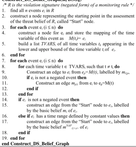
The algorithm that constructs belief graphs is shown in Figure 3. Initially, this algorithm constructs a
start node to represent the starting point of the accumulation of evidence at runtime (see line 2). Then for each event in the rule, it constructs a node to represent the occurrence of the event at runtime (line 4) and identifies the dependencies of the event to other
events (line 5). An event Ej is taken to depend on all
other events Ei whose time variables appear in the
expressions that define the lower and upper bound of
the time variable of Ej. Based on these dependencies,
the algorithm creates a directed edge from all the events
Eithat Ej depends on towards Ej (see line 9). These
edges indicate the paths for obtaining a basic belief for
Ejwhen any of the events Eiis observed. Also an
opposite edge from Ej to each of the eventsEi is created
if Ejis not a negated event (see lines 10-12). The latter
edges are used when Ejis observed before the events Ei
and indicate how the basic belief in events Eican be
computedfrom Ej.
Construct_DS_Belief_Graph(R, DSGR)
/* R is the violation signature (negated form) of a monitoring rule */
1. find all n events ei in R
2. construct a node representing the starting point in the assessment of the threat belief of R, called “Start” node.
3. for each event ei (i ≤ n)do
4. construct a node for ei and store the mapping of the time
variable of this event as M(ti)= ei
5. build a list TVARSi of all time variables tk appearing in the
lower and upper bound of the time variable ti of ei.
6. end for
7. for each event ei (i ≤ n)do
8. for each time variable t ∈ TVARSi such that t ≠ tido
9. Construct an edge to ei from ep=M(t), labelled by mi|p,
10. if ei is not a negated event then
11. Construct an edge mp|i from ei to ep=M(t)
12. end if
13. end for
14. ifei is not a negated event then
15. construct an edge from the “Start” node to ei, labelled
by the basic belief mi of ei.
16. else if ei has a time range defined by constant values then
17. construct an edge from the “Start” node to ei, labelled
[image:7.595.67.289.388.627.2] [image:7.595.309.524.404.522.2]by the basicbelief mNAF i|<x> of ei
18. end if
19. end for
end Construct_DS_Belief_Graph
Figure 3. Algorithm for constructing DS belief graphs
Note that no backward edges are constructed from
an event Ejto the eventsthat this event depends on if Ej
is a negated event (see condition in line 10). This is because negated events can only be derived through the application of the NAF principle when their ranges have fully determined boundaries. Fully determined
boundaries, however, will not be possible to have for Ej
unlessEihas already occurred. Hence, it will not be
possible to derive the truth value of Ejbefore thatof Ei
and, therefore, compute a basic belief for the latter
event based on the basic belief of the former.The label
attached by the algorithm on an edge from an event Ei
to an event Ej is the basic conditional belief function
mi|j, i.e., the function that provides the basic degree of
belief in the potential occurrence (or not) of Ej given
that Ei has already occurred.
Following the generation of edges between events,
the algorithm constructs edges from the Start node of
the graph to the nodes representing the non negated
events of the rule (see lines 14−20). These edges are
labelled by the basic belief function for the genuineness
of the event Ei that they point to. Negated events, on the
other hand, are linked with the Start node only if they
have a time range defined by constant values in the rule and, therefore, it is possible to establish their absence or not prior the seeing any other event at runtime (see conditions in lines 14 and 17). The edge linking the
Start node with a negated event Ei is labelled by the
basic belief function mNAF
i|<x>. This function is partially
determined and bound to the identifier of the specific
event Ej that triggers the application of the NAF
principle to derive the absence of Eicreating a fully
determined function mNAF
i|j for estimating the basic
belief in ¬Ei.
Figure 4. Belief graph for Rule 1
An example of a DS belief graph is shown in Figure 4. The graph represents the different paths of combining
the basic belief functions for the events of Rule 1 and
reflects the time dependencies between the different
events. The occurrence of E2 in the rule, for instance,
depends on the occurrence of E1 since the range of the
time variable of E2 (i.e., ℜ(t1,t2)) refers to the time
variable of E1 but not vice versa (the range ℜ(t1,t1) of t1
indicates that E1 is an event with a not constrained time
variable). Thus, an edge from E1 to E2 labelled by m2|1
has been inserted in the graph as well as another edge
from E2 to E1 labelled by m1|2. Similarly, as the time
range of the event ¬E3(i.e., ℜ(t1+1,t2−1)) refers to the
time variables t1 and t2 of the events E1 and E2, the
graph contains edges from E1 to ¬E3and E2 to ¬E3.
Note, however, that the graph does not contain an edge
from ¬E3to E2or from ¬E3to E1 as the former event
cannot be derived by NAF unless E1and E2are received
E1 E2
S
m2|1 m3|2
m1|2
m2
m1
¬E3
first. Finally, the graph includes edges from the starting
node to E1 and E2. These edges are labelled by m1 and
m2 representing the basic belief functions that are to be
used when the occurrence or absence of the events E1 or
E2 is established from the starting node.
At runtime, belief graphs are used to record the events matched with a given rule and determine the combination(s) of basic belief functions that will be needed to compute the overall threat belief for the rule. In general, given a set of received and a set of unknown events, the overall belief for a rule is evaluated by combining the basic beliefs of the received events that match with the rule’s violation signature and the conditional beliefs for the unknown events. It should be noted that in such cases, there may be more than one known events in the graph which are linked directly with an unknown one. If this is the case, the conditional
belief in the unknown event mi|j is computed by
considering all paths which start from some known
event Ei and end in the unknown event Ej, without
passing through any other known events (this ensures that known events will not be considered as supporting evidence for unknown ones multiple times). The algorithm for evaluating the overall belief in a rule threat given a belief graph is shown in Figure 5.
Compute_Threat_Belief(Ei, DSGR, R)
1. find the sets of the known events KE and the set of the
unknown events UE in DSGR
2. m = basic_belief (<start, Ei>)
3. CombinedBPA = {}
/* combine the basic beliefs of events in KE */
4. for each Ek in KE do
5. m = m ⊕ basic_belief (<start, Ek>)
6. CombinedBPA = CombinedBPA ∪ basic_belief (<start,
Ek>)
7. end for
8. for each ej ∈ UE do
9. insert all the paths from ei to ej, which do not include any
event in KE, into Pij
10. for each p ∈ Pijdo
/* combine the BPAs of paths to unknown events */
11. for each edge L in p do
12. if basic_belief (L) ∉ CombinedBPA then
13. m = m ⊕ basic_belief (L)
14. CombinedBPA = CombinedBPA ∪
basic_belief (L)
15. end if
16. end for
17. end for
18. end for
19. mark Ei as a known event in DSGR
20. return (m(events(¬R), m(events(R)))
end Compute_Threat_Belief
Figure 5. Algorithm for computing overall threat belief
To demonstrate the estimation of the threat beliefs
consider Rule 1 again and the following sequence of
events:
• Happens(e(e100,Lap30,Lap30,REQ,
login(User1,Lap30),Lap20),80,ℜ(80,80))
• Happens(e(e101,Lap2,Lap2,REQ,
login(User1,Lap2),Lap2),87,ℜ(87,87))
When it arrives at EVEREST, the first of these
events (e100) can be matched with the nodes E1 or E2
of the belief graph of Figure 4. Each of these matches produces a separate instantiation of the belief graph and leads to the estimation of different threat beliefs. When
matching e100 with node E1, for instance, the threat
belief will be computed by the combination of the basic
belief functions (m1 ⊕ m2|1) ⊕ m3|1. Based on the
definition of these functions in Section IV, it can be shown that the application of the rule of the orthogonal
sum will result in the following functional form for (m1
⊕ m2|1) ⊕ m3|2:
) 1 ( ) 1 ( ( 1 ) 1 ( ) 1 ( )) ( ( ' 1 ' 21 ' 31 ' 1 ' 21 ' 31 ' 1 1 21 ' 31 ' 21 21 1 ' 31 1 21 ' 31 3 2 1 1 | 3 1 | 2 1 k k k k k k k k k k k k k k k k k E E E m m m − + − − − − + − − + = ¬ ∧ ∧ ⊕ ⊕
Thus, if we assume that: (i) the basic belief in the
genuineness and non genuineness of e100 are k1 = 0.8
and k1’ = 0.1, respectively (note that the sum of these
two beliefs may be less than 1 in the DS theory); (ii) the basic conditional belief in observing or not a second genuine login event within 100 time units after
the observation of e100 are k21 = 0.6 and k21’ = 0.4,
respectively; and (iii) the conditional basic belief in not observing a genuine logout event in the period of 100
time units between two genuine login events are k31 =
0.2 and k31’=0.6, respectively, the overall threat belief
for the first instance of the rule will be:
45 . 0 ) 9 . 0 * 4 . 0 * 6 . 0 9 . 0 * 4 . 0 * 2 . 0 ( * 1 1 * 6 . 0 * 6 . 0 0 * 8 . 0 * 6 . 0 8 . 0 * 6 . 0 * 6 . 0 )) (
( 1 21| 3|1 1 2 3
= + + + = ¬ ∧ ∧ ⊕
⊕m m E E E
m
The threat belief for the same rule instance will be
updated when the event e101 arrives. Upon its arrival,
e101 will be matched with the node E2 in the belief
graph instance. Thus, according to the
Compute_Threat_Likelihood algorithm, the overall threat belief will be estimated by the combination of the
basic belief functions (m1⊕m2)⊕m3|2, which due to the
rule of the orthogonal sum will be:
) 1 ( ) 1 ( ( 1 ) 1 ( ) 1 ( )) ( ) ( ' 1 ' 2 ' 31 ' 1 ' 2 ' 31 ' 1 1 2 ' 31 ' 2 2 1 ' 31 1 2 ' 31 3 2 1 2 | 3 2 1 k k k k k k k k k k k k k k k k k E E E m m m − + − − − − + − − + = ¬ ∧ ∧ ⊕ ⊕
Thus, if the basic belief assignments in the
genuineness of e101 (i.e., m2(Genuine(e101,…)) and the
non genuineness of this event (i.e.,
m2(¬Genuine(e101,…)) are k2 =0.8 and k2’ = 0.2
respectively, and the overall threat likelihood will be:
54 . 0 ) ( )
(m1⊕m2 ⊗m3|2 E1∧E2∧¬E3 =
The increase in the overall threat belief in this case
is due to the fact that the basic belief in E2 given by
m2(X) is higher than the basic belief in E2 that is
VI. EVALUATION
The threat detection tool of EVEREST has undergone a preliminary evaluation whose objective was to estimate the timeliness and precision of the threat detection signals generated by the tool. This
evaluation was based on the simulation of a location
based access control system (LBACS) that grants access to the computational resources of an enterprise (e.g., printers, intranet) from mobile devices, depending on the credentials of these devices and their exact location within the physical space of the enterprise.
In the evaluation, timeliness was measured by the threat reaction time (TRT) of each threat signal. TRT was defined as the difference between the time when the monitor of EVEREST detected a violation of a
monitoring rule (Tmon) and the time when TDT
produced a threat signal corresponding to the same violation (Ttd), i.e.,
TRT = Tmon− Ttd
Precision was defined as the proportion of the threat signals generated by TDT within a given range of threat belief values (BR) that corresponded to definite eventual violations of the relevant rules and measured by the formula:
PR = TTSBR /(TTSBR + FTSBR)
In this formula, TTSBR is the number of the threat
signals with a belief in a given range (BR) that corresponded to eventual violations of the relevant rule detected by the EVEREST monitor (true signals), and
FTSBR is the number of the threat signals with belief in
a given range (BR) that did not correspond to an eventual violation of the relevant rule. Our focus on precision and timeliness was because the former of these measures indicates the accuracy of the threat detection signals and the latter indicates the time that is available for reaction before the definite violation of an monitoring rule is detected.
For the evaluation we executed 8 different experiments having 2000 events each. The events for each experiment were generated randomly by simulating the workflow of LBACS, assuming that the event inter-arrival time had a normal distribution with a mean of 1 second and a variance of 0.3, 0.6, and 0.9 seconds. The different variance values (VV) were used to create different event sets that imposed different stress conditions for the monitor (the smaller the VV the more stressing the monitoring conditions). The eight experiments varied also in terms of the used size of the diagnosis window (DW) and event sample size (SS)
(i.e., the size of the set Log(Ej) in the computation of
the mi|j conditional beliefs) as shown in Table 2. The
monitoring rules that were used in the experiments to detect threats are described in detail in [13].
D. Threat reaction time
Table 2 shows the minimum, maximum and average timeliness measures for S&D threat detection in the different experiments (in seconds) as well as the
proportion of S&D threat signals with positive and
negative timeliness measures (see columns pos (%) and
[image:9.595.306.531.166.292.2]neg (%), respectively). A negative time period indicates that TDT computed its threat belief after a threat occurring and vice versa.
Table 2 Threat reaction time (secs)
EXP VV DW SS pos %
neg %
ave TRT
max TRT
min TRT
1 0.3 15000 10 77.54 21.51 9.3 852.5 -4.2 2 0.3 20000 15 73.21 26.53 10.4 753.9 -4.5 3 0.5 15000 10 80.18 19.02 12.5 1137.0 -1.9 4 0.5 20000 15 72.08 27.39 13.2 1110.7 -3 5 0.6 15000 10 79.45 20.03 12.3 1077.2 -2.3 6 0.6 20000 15 74.87 24.74 14.0 1077.2 -29 7 0.9 15000 10 80.24 18.85 13.6 1077.2 -3 8 0.9 20000 15 74.87 24.74 14.1 1077.2 -29
As shown in the table, in 70% to 80% of the cases S&D threat detection signals were produced prior to the actual violations and the mean reaction time of these signals ranged from 9.3 to 14.1 seconds. These results indicate that on average the detection of S&D threats was timely and provided scope for triggering automatic preventive actions for violations (e.g., deactivate the component that causes the problem or block any further interactions with it).
E. Precision
Figure 6 shows the average, maximum and minimum precision measures for the threat signals generated for different monitoring rules in the different
experiments (see the series AvePR, MaxPR and MinPR,
respectively).
Precision
76 77 78 79 80 81 82 83
1 2 3 4 5 6 7 8
Experiment
Pr
e
c
is
io
n Min PR (%)
[image:9.595.310.524.476.588.2]Ave PR (%) Max PR (%)
Figure 6. Precision of threat signals
DW and SS were increased. This can be evidenced by
contrasting the precision measures of exp 1 and exp 2,
exp 3 and exp 4, exp 5 and exp 6, and exp 7 and exp 8
(these experiment pairs vary in terms of the size of DW and SS but have the same VR as shown in Table 2). This effect of DW and SS on precision was expected as larger DW and ES provided a wider evidence basis for estimating more accurate beliefs. It should, however, be noted that in no case the increase in precision due to increases in DW and ES was larger than 1.8% (i.e., the
largest increase that was observed in the case of exp 7
and exp8). Hence, our approach is not overly sensitive
to DW and ES.
VII. RELATED WORK
Our approach to threat detection is related to
intrusion detection [2][7]. Most intrusion detection systems, however, only detect malicious actions that have already happened (intrusions) whilst our approach to threat detection tries to predict violations.
Approaches to intrusion detection are classified as
anomaly-based or misuse-based [7]. Anomaly-based approaches [1][2][4] assume that attacks involve, somehow, abnormal behaviour of the system, and threats and intrusions are detected as deviations from normality. Misuse-based approaches [3][6][9], on the other hand, are based on models of known attacks. The threat detection approach presented here is essentially
anomaly-based. In particular, it is model or
specification-based [1][4] as threats and intrusions are detected as deviations from a model of the normal behaviour of the system. Our approach is similar to [1] in protecting system assets and building monitoring policies with the goal of protecting them.
Our approach has also characteristics of misuse-based techniques. This is because it detects threats from rule violation signatures, which could be viewed
as an attack model. It should be noted, however, that
we do not assume a complete attack model as, for example, in [14]. Furthermore, the detection of threats (potential attacks) in our approach is probabilistic and is not based on model checking (as in [14]) or logic-based reasoning techniques. Finally, we should note that our approach is related to statistical attack detection approaches which are based on Bayesian networks (e.g., [9]), although it uses the alternative DS theory for the reasons we discussed in Section IV.
VIII.CONCLUSIONS
In this paper, we have described an approach for the runtime detection of S&D threats that we have implemented as part of the EVEREST monitoring framework. In this approach, when some runtime event instantiates a monitoring rule expressing an S&D property and can, therefore, possibly lead to a violation of the rule, the event constitutes an S&D threat. To
enable concentration on S@D threats which are more likely occur in some future state in the operation of a system, our approach calculates the likelihood of a potential violation of the given rule based on evidence regarding the genuineness of the relevant events and historical data about event co-occurrences. The actual computations are based on basic belief functions grounded in the DS theory of evidence. Our threat detection approach has been implemented as an extension of EVEREST and an initial empirical evaluation of it has been carried out with positive results.
Ongoing work focuses on the exploitation of non time variable constraints between events whilst computing conditional basic beliefs in event occurrence. We are also evaluating the merit of our approach in predicting violations of non S&D properties for service based systems, as part of the EU F7 project SLA@SOI. Our work in the latter area is also concerned with the prediction of aggregate properties (e.g., average service availability).
IX.REFERENCES
[1] Chari, S.N. and Cheng, P.-C., “Bluebox: a policy-driven, host-based intrusion detection system”, ACM Transactions on Information Systems Security 6(2):173-200, 2003.
[2] Denning, D. “An Intrusion Detection Model”, IEEE
Transactions on Software Engineering, 13(2): 222-232, 1987. [3] Ilgun, K., R.A. Kemmerer, and P.A. Porras, “State transition analysis: a rule-based intrusion detection system”, IEEE Transactions on Software Engineering, 21(3):191-199, 1995
[4] Spanoudakis G, Kloukinas C. Mahbub K., “The SERENITY
Runtime Monitoring Framework”, In Security and Dependability for Ambient Intelligence, (eds) Spanoudakis G., Mana A., Kokolakis, Information Security Series, Springer, pp. 213-238, 2009
[5] Ko, C., M. Ruschitzka, and K. Levitt. “Execution monitoring of security-critical programs in distributed systems: a Specification-based approach”. IEEE Symp. on Security and Privacy, 1997. [6] Kumar, S. and E.H. Spafford. “A Pattern Matching Model for Misuse Intrusion Detection”. In 17th National Computer Security
Conference, pp. 11-21, 1994.
[7] Lazarevic, A., Kumar, V., Srivastava, J. “Intrusion detection: a survey”, In Managing cyber-threats: issues approaches & challenges, Springer, 2005.
[8] Spanoudakis, G., Mahbub, K., “Non intrusive monitoring of service based systems”, Int. J. of Cooperative Inform. Systems, 15(3):325–358, 2006.
[9] Valdes, A. and K. Skinner Adaptive, “Model-based
Monitoring for Cyber Attack Detection”. In Recent Advances in Intrusion Detection, pp. 80-92, 2000.
[10] Shanahan M. P. “The Event Calculus explained”. In Artificial Intelligence Today, LNAI 1600:409–430, 1999.
[11] Spanoudakis G., Tsigkritis T., Kloukinas C., “2nd Version of
Diagnosis Prototype”, Deliverable A4.D5.2, SERENITY Project, http://www.serenity-forum.org, 2009.
[12] Shafer G., “A Mathematical Theory of Evidence”, Princeton University Press, 1975
[13] Armenteros-Pacheco A. et al, “Evaluation of the SERENITY framework v2”, Deliverable A7.D5.4, SERENITY Project, http://www.serenity-forum.org, 2009