Bayesian latent variable models for collaborative item rating prediction

Bayesian Latent Variable Models for Collaborative Item

Rating Prediction

Morgan Harvey

_{, Mark J. Carman}

_{, Ian Ruthven}

_{and Fabio Crestani}

2_{Faculty of Informatics, Monash University, Melbourne, Australia} 3

Department of Computer Science, Strathclyde University, Glasgow, Scotland 4_{Faculty of Informatics, University of Lugano, Lugano, Switzerland}

[email protected]

ABSTRACT

Collaborative filtering systems based on ratings make it eas-ier for users to find content of interest on the Web and as such they constitute an area of much research. In this paper we first present a Bayesian latent variable model for rat-ing prediction that models ratrat-ings over each user’s latent interests and also each item’s latent topics. We describe a Gibbs sampling procedure that can be used to estimate its parameters and show by experiment that it is competitive with the gradient descent SVD methods commonly used in state-of-the-art systems. We then proceed to make an im-portant and novel extension to this model, enhancing it with user-dependent and item-dependant biases to significantly improve rating estimation.

We show by experiment on a large set of real ratings data that these models are able to outperform 3 common base-lines, including a very competitive and modern SVD-based model. Furthermore we illustrate other advantages of our approach beyond simply its ability to provide more accu-rate ratings and show that it is able to perform better on the common and important case where the user profile is short.

Categories and Subject Descriptors

H.3.3 [Information Storage & Retrieval]: Information Search & Retrieval

General Terms

Algorithms, Experimentation, Performance

Keywords

Recommender systems, Topic Models, User modelling

Permission to make digital or hard copies of all or part of this work for personal or classroom use is granted without fee provided that copies are not made or distributed for profit or commercial advantage and that copies bear this notice and the full citation on the first page. To copy otherwise, to republish, to post on servers or to redistribute to lists, requires prior specific permission and/or a fee.

CIKM’11,October 24–28, 2011, Glasgow, Scotland, UK. Copyright 2011 ACM 978-1-4503-0717-8/11/10 ...$10.00.

1.

INTRODUCTION

The sheer number of items available in online systems can be overwhelming for users and makes finding items of interest extremely challenging. Furthermore the rapid and continual expansion of the Web makes it impossible to man-ually evaluate each new item to determine if it might be of interest. Content filtering systems, based on techniques from information retrieval, are designed to assist in this pro-cess by narrowing down the number of items a user has to look through in order to fulfil a particular information need. These systems rely on textual descriptions of items and seek to match these descriptions with a user’s profile in order to suggest useful items. One significant issue with this content-based filtering is that for some types of items it can be extremely difficult to choose suitable descriptive terms to search for.

Another, more accurate, approach to discovering items of interest is provided by ratings-based collaborative filtering systems, which use past ratings to predict items the user may like. Such systems predict which items a given user will be interested in based on the information provided in their user profile. These profiles consist of votes or ratings for items in the system that the user has already viewed and evaluated. The profiles of other users are frequently also exploited to improve predictions for the target user.

Profiles are generally constructed explicitly from user rat-ings, however they may also be compiled implicitly by con-sidering a user’s purchase or bookmark history. Explicit rat-ings systems are commonly found on movie and music rec-ommendation sites such as MovieLens [14] or imdb where users can give each item a rating from 0 to 5 stars. Zero indicates that the user strongly dislikes the item and five indicates that they really like the item, however any dis-crete set of values could be used. Implicit systems can also be used, for example in online retail stores such as Amazon [12] where users purchase items or add them to a “wish list”, indicating that they are interested in that kind of item.

simply ordering unrated items in descending order of their predicted rating. In doing so, such an algorithm is effectively achieving two outcomes: the “forced prediction” of whether or not a user will have a preference for an item and the “free prediction” of the expected rating itself.

In this work we focus on the problem of recommending items to users based purely on the explicit ratings they have assigned to other items in the system. We introduce 2 novel (and related) Bayesian probabilistic models designed to ac-curately predict ratings given the very sparse training data commonly found on e-commerce and recommendation web sites. We go on to show by experiment with a large set of real ratings data that our models are able to outperform 3 common baselines, including a very competitive and modern SVD-based model. Furthermore we illustrate a number of other advantages of our approach, beyond simply its ability to provide more accurate ratings.

The rest of the paper is structured as follows: we first dis-cuss some relevant related work in the field of collaborative filtering and describe how the majority of modern methods approach the problem. In section 3 we describe the rating estimation problem in more detail and outline common mea-sures for algorithm performance. In section 4 we introduce a pair of novel Bayesian models designed to decompose the problem by use of latent factors and describe how these mod-els can be used to estimate unknown ratings. In sections 5 and 6 we describe experiments conducted with a large data set of 10 million movie ratings comparing the performance of these new models to 3 appropriate baselines and discuss the result of these experiments. Finally we offer our conclud-ing remarks and make suggestions of possible future work building upon the results of this paper.

2.

RELATED WORK

Collaborative filtering systems can be placed in the con-text of information retrieval by considering that in a retrieval system items are “pulled” by users through the issuing of ex-plicit search queries. Filtering systems on the other hand are described as “push” systems since they quite literally push items at a user that is predicted he/she will like. Much early work was done in the 90s and the field has seen a resurgence of interest lately, primarily due to the Netflix prize [11]. Col-laborative filtering algorithms can be generally classified into 2 distinct types: memory-based and model-based.

2.1

Memory-based CF

Early systems were memory-based and made use of the original ratings matrix to formulate predictions. Such sys-tems follow a relatively simple 2 step process: First they identify a neighbourhood of users similar to the target user and then use an aggregate weighted summation of the neigh-bours’ ratings for an item in order to predict the rating for the target user. These algorithms form the basis of most fil-tering currently performed on the Web including sites such as Amazon and CDNow and were the cornerstone of much early research in the field [7, 4]. We refer to [1] for a com-prehensive description of how these methods operate. It has been speculated that their popularity is due to their relative simplicity and their inherently intuitive nature [10].

Unfortunately these simple, memory-based algorithms suf-fer from 2 major shortcomings. Firstly the number of items rated by most users is oftentimes small and therefore it can be difficult to choose a good neighbourhood of similar users.

Once a neighbourhood is chosen only a very small number of similar users may have rated the item for which we wish to predict a rating. Secondly, these algorithms require all of the ratings data to be utilised when making a prediction and, although it is possible to maintain a cache of user sim-ilarities, this will have to be updated whenever new ratings are made. This shortcoming is perhaps the most problem-atic as without clever implementation, it severely restricts the potential growth of the recommendation system. This is because, over time the amount of ratings data becomes too large to allow for the efficient computation of both the neighbourhoods and the predictions themselves.

2.2

Model-based CF

These issues led to the development of the second general type of collaborative filtering algorithm: the model-based approach. In this approach we use the observed ratings to construct a model of the data and we decompose the ob-served ratings into a sum of biases; one for the user, one for the item and a third joint bias. Modern examples of these models frequently use some form of dimensionality reduc-tion to uncover latent factors and to calculate the joint bias. These latent factors are constructed in a manner that best explains the training ratings and if we make the assumption that any further ratings will be drawn IID1 from the same distribution then the model should be able to predict new ratings well.

These model-based algorithms are able to overcome many of the scalability problems associated with the earlier memory-based systems. This is particularly the case when real-time recommendations are required, which is obviously the most likely situation given the on-line nature of the systems where collaborative filtering is most often used. The most time-consuming task is the generation of the model itself, after which the task of new predictions is extremely quick due to the significant reduction in dimensionality afforded by the latent factors. With model-based systems the entire mod-eling operation can be completed off-line thus allowing for near-instantaneous real-time predictions as and when users need them.

Many examples of this approach, including most attempts at the Netflix prize, use gradient descent algorithms to esti-mate an approximation of the Singular Value Decomposition (SVD) of the original sparse ratings matrix [15]. The val-ues computed for the SVD matrices are regularised so as to prevent over-fitting and individual biases for each user and movie are commonly added to improve prediction perfor-mance. Other techniques use probability theory to construct the models where observed ratings are assumed to arise from some latent variables which have to be estimated. In [13], Marlin represents each user as a mixture of “attitudes” with each rating being generated by selecting one of these atti-tudes and then selecting the rating based on the ratings dis-tribution for that attitude. Hofmann [10] extends his earlier pLSI model to model ratings by again assuming that users have a distribution over “interests” or “attitudes” and that each rating is associated with a single interest drawn from the user’s interest distribution. His work differs from that of Marlin [13] however by then assuming that there is a rating distribution for each latent interest and item pair. So the observed rating is assumed conditional on both the latent

1

interest of the user who rated the item and also on the item itself.

Other probabilistic approaches include [19] in which the authors introduce a novel adaptation of the EM algorithm to learn the parameters of a prediction model for person-alised content-based prediction. Stern et. al. [17] instead use Expectation Propagation and Variational Message Pass-ing to learn a model usPass-ing both ratPass-ings data and content. In other recent work Chen et al. [5] compare the performance of Latent Dirichlet Allocation (LDA) [2] with association rule mining (ARM) for the purpose of community recommen-dation. This is a similar problem to rating prediction but instead involves the suggestion of online communities of in-terest rather than items. They show that LDA consistently outperforms ARM for this task, particularly when consider-ing later recommendation. They also demonstrate that it is less likely to make extreme errors due to its Bayesian nature, certainly a useful property when recommending items.

In this paper we discuss 2 probabilistic model-based col-laborative filtering algorithms that can be seen as compara-ble to these models and draw on similar background theory. Blei [2] in fact uses collaborative filtering as an example of a problem for which LDA could be used and shows that it is able to outperform both probabilistic LSA [9] and a sim-ple unigram model. Our models do not use LDA itself in order to predict ratings but use its ability to extrude latent factors from sparse data as a strong basis from which to build models more suited to the task at hand. Also in this work we extend the basic ratings model by including indi-vidual biases for each user and item requiring an iterative fixed-point optimisation procedure to be interleaved with the Gibbs sampler and providing significant improvements in performance.

3.

PROBLEM DEFINITION

Before proceeding any further we will formally define the problem of rating prediction and describe the format of the data we have to work with. We have a set of users of the systemU={u1, . . . ,uU}, a set of itemsM={m1, . . . ,mM} and a discrete set of possible ratings{1, . . . ,R}. Our training data is a collection of ratings given by the users to items. We can view each individual rating as a tuple: (ui, mi, ri) fori:= 1. . . Ntrain. For example the tuple (ui = 1, mi = 1, ri = 4) would indicate that user 1 had given item 1 a rating of 4. It can sometimes be convenient to visualise the complete collection of user ratings as a large and very sparse matrixRof sizeU×M whererumwould indicate the rating given by useruto itemm. The prediction problem is best described by saying that we would like to “fill in” the sparse ratings matrix, extrapolating (or predicting) a rating ˆrumfor every possible user-item pair from the limited data available. More practically we wish to define some function or model which will minimise the root mean squared prediction error over the test data:

RM SE=

v u u

t 1

Ntest Ntest

X

i=1

(ri−ˆri)2 ₍₁₎

The RMSE is commonly used in statistics for measuring the difference between the set of values predicted by a model and the values actually observed from the system being mod-elled. It is a good measure of precision and is an unbiased estimator of the standard deviation of the predictions and

α

_β

θ

ϕ

r

N

z

u

m

b

YZ

y

σ

μ

b

M

b

U

α

β

θ

ϕ

U

r

N

z

u

m

b

YZ

y

M

σ

μ

α

_β

θ

ϕ

r

N

z

u

m

b

YZ

y

σ

μ

b

M

b

U

α

β

θ

ϕ

U

r

N

z

u

m

b

YZ

y

M

σ

μ

Figure 1: Latent Interest and Topic Ratings Model (LITR) where each observed change in the rating from the mean is due to both a user interest and an item topic or genre and Biased-LITR (BLITR) where it is also dependent on the bias for the user and the item.

is therefore a good choice of error function for collaborative filtering. We also report the Mean Absolute Error (MAE) which is simply the mean absolute difference between the predicted rating and the actual rating, over the whole test set.

4.

LATENT INTEREST AND TOPIC

RAT-INGS MODELS

Symbol Description

M number of items U number of users N number of ratings Y number of topics/genres Z number of user interests ri rating at positioni

mi item for rating at positioni

ui user who contributed rating at positioni yi topic/genre allocation at positioni zi user interest allocation at positioni ˆ

rum predicted rating for useruand itemm φm distribution over topics for itemm θu distribution over interests for useru bm bias due to itemm

bu bias due to useru

byz bias due to interest/topic pairyz α parameter of Dirichlet prior over Θ β parameter of Dirichlet prior over Φ ρ smoothing parameter for bias estimates σ standard deviation over all ratings

µ mean rating

Table 1: List of notation for Ratings Models

the vocabulary. Each word positioniin the document col-lection is assigned a latent random variablezi which ranges over the latent topics.

The model possesses a number of advantageous attributes; it is fully generative meaning that it is easy to make infer-ences on new documents and its Bayesian nature helps to overcome the over-fitting problem present in models such as Probabilistic Latent Semantic Indexing (pLSI) [9]. Also since in LDA each document is a mixture of topics it is far more flexible than models that assume each document is only drawn from a single topic. These advantages also extend to models based on LDA with both the added flexibility and ability to easily incorporate new data being very important for our own models, as we shall discuss later. Many useful models have used LDA as a base to work from, for example the Author-Topic model [18] which models academic pub-lications and citations. It has even been used to develop models to annotate images based on their visual features [3].

As we can see from these publications, LDA can serve as a very flexible starting point for more complex models even when those models are not just using discrete data. In the case of collaborative filtering we do not have documents and terms, but rather a collection of observed ratings from a set of users over a set of items. We must therefore significantly adapt the model to fit the problem. Since we are primarily interested in predicting ratings with the smallest possible er-ror in aggregate it is sensible to consider models (and there-fore distributions) that are continuous in nature. In doing so the predictions will not be constrained to be bound to the finite discrete values of the original ratings but will have the freedom to model the complex interactions of biases in the data at higher granularity.

4.1

Basic Generative Model

Perhaps the simplest possible prediction algorithm one could imagine would be to assign the mean rating over the training data, denoted µ (where ˆµ = 1

N P

iri), as a pre-diction to each item for every user, (i.e. ˆrum =µ). This overly simplistic model corresponds to a generative process in which each ratingriis considered a normally distributed random variable with meanµand standard deviationσ:

ri ∼ N(µ, σ2) (2)

This model makes a large number of assumptions and ig-nores a lot of the complexity in the data. It assumes that ratings are completely independent of both the item and user and that there are no interactions between the combi-nations of user and item that would affect the rating. We relax some of these assumptions and extend this model by following similar conclusions to both Hofmann [10] and Mar-lin [13]. That is that the change in the rating is dependent on the user and that each user can be characterised by a distribution over a small number of latent interests.

In addition, (and in contrast to previous work) we then as-sume that the change in rating is also equally dependent on the items, which themselves can be characterised by a distri-bution over a small number of latent topics. For example in the case of movies this may be more intuitively thought of as their latent genres or for general items in a web store it could be the category/ies to which they could be assigned. This conjecture leads to a more useful generative model for per-sonalised item filtering and ranking involving three random variables: a user interestzi, an item topic (or movie genre) yi and a ratingri, where only the last variable, the rating itself, is observed. Following previous work on topic models, we then assume the user-interest and item-topic variables are drawn from Multinomial distributions.2 The same as-sumption could also be made regarding the ratings, as the original ratings assigned by users are indeed drawn from a discrete set. However as noted earlier, the flexibility of the model can be increased as can the granularity of its predic-tions, by instead modelling them as being drawn from Nor-mal distributions. These assumptions can be summarised as follows:

zi ∼ M ult(θui) (3)

yi ∼ M ult(φm_i) (4)

ri ∼ N(µ+by_izi, σ 2

) (5)

Thus the model consists of a discrete probability distribu-tion over interests for each user θu, a discrete distribution over topics for each itemφm, a mean ratingµ, a bias value byz for every pair of interests and topics, and a standard deviation parameterσ. A graphical model corresponding to this generative process is shown at the top of Figure 1.

The intuition for introducing the bias byz in this model is that we believe each interest and topic combination will have an effect on how the item is rated. For example in the case of movies we might expect that a user who likes romance would give a horror movie a lower than average rating, meaning that the biasbyz for this interest-topic pair would be negative. Similarly if the same user was to rate a romance movie then we would expect them to give a higher

2

than average rating and the bias would therefore be positive. Since these biases are calculated over the low-dimensionality latent spaces they will not be sparse and should allow the model to generalise well to unseen user-item combinations, a key objective of any collaborative filtering model.

Given suitable estimates for these parameters, we can pre-dict the rating for a useruand item m by calculating the expected value as follows:

ˆ

rum = E[r|u, m] =

X

y,z

E[r|y, z]P(y|m)P(z|u) (6)

= µ+X y,z

byzφy|mθz|u (7)

Hereθz|uandφy|mdenote probability of an interest given a user and a topic given an item respectively. This model is quite intuitive. It states that the rating given by a user to an item will be the product of a user’s affinity for an interest, the item’s probability of belonging to a topic and the average bias for that interest-topic combination, summed over all possible combinations of interests and topics.

In this model we have associated a possibly non-zero bias with every pair of interest topic dimensions. Thus not only is a positive bias associated with “corresponding”’ interests and topics (e.g. the user-interest “horror” and the movie-genre “horror”) but also a possibly negative bias with “non-corresponding”’ interests and topics. For instance if a user’s primary interest is “horror”, they may still have a positive bias towards a “thriller” while having a negative bias against a “comedy”. In SVD terms this is to some extent equivalent to replacing the diagonal singular-value matrix with a ma-trix containing non-zero off-diagonal values. These values then allow us to model both positive and negative correla-tions across different factors. By defining the prediccorrela-tions in terms of a generative model, we can interpret and explain the parameters of the model in a way that is not possible with SVD-based prediction algorithms.

4.2

Parameter Estimation

Given vectors of latent variable assignmentsz= (z1, ..., zN) andy= (y1, ..., yN), we can compute estimates of both the probability of an interest given a userθz|uand a topic given an itemφy|m. Following principles from LDA, and in keeping with Bayesian statistics, we place symmetric Dirichlet pri-ors on both of these distributions, resulting in the following expectations for the parameter values under their respective posterior distributions:

ˆ θz|u =

Nzu+α1 Z

Nu+α (8)

ˆ φy|m =

Nym+β_Y1

Nm+β (9)

HereNzu,Nym,NuandNuare counts denoting the number of times the interestz appears (in z) together with useru, the number of times topic y appears (in y) with item m, and the total ratings by useruand for itemmrespectively. Z is the number of interests andY is the number of topics. The hyperparametersαandβact as pseudo-counts, allowing the model to fall back on the (uniform) prior probability in the event of sparse data, which is particularly useful in this setting where sparse data is common.

In addition to estimating the distributions over interests

and topics we need to estimate the bias for each interest and topic pair denotedbyz. Given that we have a complete set of assignments for these latent variables for each observed ri we can calculate an estimate of this bias as follows:

ˆ

byz =

P

i:(yi=y)∧(zi=z)(ri−µ)

Nyz+ρ (10)

Here Nyz denotes the number of ratings for which y and z appear together and ρ is a smoothing parameter. It is related to the variance of the zero mean Gaussian prior on byz, which keeps the model Bayesian and helps to deal with sparsity in the data.3 We note that it would also be possible to estimate a variance parameter separately for each (y, z) pair, but we instead make the simplifying assumption that all biases have the same fixed variance.

While exact inference of latent variable models such as LITR is intractable, a number of methods of approximating the posterior distribution exist including mean field varia-tional inference [2] and Gibbs sampling [8]. Gibbs sampling is a Markov chain Monte Carlo method where a Markov chain is constructed that converges to the target distribution of interest over a number of iterations. In Gibbs sampling the next state in the chain is reached by sampling all vari-ables from their conditional distribution given the current values of all other variables [6].

Gibbs sampling for this model involves sampling first zi and then yi for each rating ri. To sample for zi we cal-culate distribution P(z|ri, yi, ui, µ, σ,z−i), which is condi-tioned on the current assignment to all interest variables exceptzi. Similarly foryi we sample from the distribution P(y|ri, zi, mi, µ, σ,y−i). Note that our estimates for the pa-rametersθz|u,φy|mandbyzdepend on the interest and topic assignments z and y, so when calculating estimates using Equations 8, 9 and 10, we simply remove theithrating from the sample. The conditional probability distributions are then estimated as follows:

P(z|ri, ...) ∝ p(ri|yi, z)P(z|ui)

∝ exp

(ri−(µ+byiz)) 2 σ2

_Nzu+α1

Z Nu+α (11) P(y|ri, ...) ∝ p(ri|y, zi)P(y|mi)

∝ exp

(ri−(µ+byz_i))2 σ2

_Nym+β1

Y Nm+β (12)

Herep(r|y, z) denotes the conditional probability density at ratingr for the interestyand topicz. Since the algorithm only require estimates proportional to the true probabilities the normalising factor of the Normal distribution is not re-quired. Therefore the first parts of Equations 11 and 12 are the unnormalised probabilities of a Normal distribution. This model provides a method of predicting ratings by con-sidering perturbations from the mean rating over a number of latent interests and topics.

After sufficient iterations of the sampler, the Markov chain converges and the parameters of the model can then be esti-mated from the assignmentszandyvia equations 8 and 9. For increased accuracy, we average parameter estimates over consecutive samples from the Markov chain. Gibbs sampling is a preferable alternative to methods such as Expectation

Maximisation as it is able to sample from the entire pos-terior distribution and is therefore unlikely to get “stuck” in local maxima and does not require the use of additional machinery such as simulated annealing to get around this problem [16]. Another benefit of this technique is the ability to quickly “fold-in” new data into the model, this is partic-ularly useful for this task as new ratings, items and users are likely to appear quite frequently. To include this new data into the model we can simply run the Gibbs sampler over the new data, holding all of the pre-existing interest and topic allocations fixed. After the sampler has converged on this new data (which usually occurs within less than 50 iterations) we can simply recalculate parameter estimates in equations 8 and 9.

4.3

Adding User and Movie Biases

As noted in section 2, the most successful models compet-ing in the Netflix prize also estimate a bias for each user and a bias for each item as well as the bias due to the user and the item together. This is a sensible assumption as some users may naturally rate items higher than others and some may naturally choose from a lower baseline score. Simi-larly some items are intrinsically better than others and are therefore likely to be rated higher by all users, while items of a lesser quality will be given a lower than average score by most users. While we would expect that these biases would be at least partially accounted for by the joint biases over the reduced genre and interest spaces it is likely that users and movies that give/have unusually high or low rat-ings (outliers) would affect the accuracy of the biases for other users. By calculating a separate bias for each user and item separately we effectively remove these eccentrici-ties from the ratings, giving the joint biases the freedom to deal purely with the variations caused by observing the var-ious interest/genre pairs. The Biased-LITR model (BLITR) is therefore an extension of the model described previously to also include these biases in order to improve prediction accuracy. The graphical representation for this model is on the bottom in Figure 1.

The generative model is the same as the previous case, except that the mean of the Gaussian distribution that gen-erates the rating ri takes into account the user and item biasesbu_i andbm_i as follows:

ri ∼ N(µ+bui+bmi+byizi, σ 2

) (13)

Given estimates for the parameters of this more compli-cated model, the predicted rating for a useruand an item mis now:

ˆ

rum=_E[r|u, m] =µ+bu+bm+X y,z

byzφy|mθz|u (14)

Note that the prediction under this new model and the previous model can be viewed as perturbing the mean µ by a combination of biases. Both models add a bias for the likely interests and topics given the user and item pair, while the second model adds also explicit biases for the user and for the item.

Estimates for the parametersθz|u andφy|mare the same as in the previous model, while the estimate forbyz must now include the effects of the extra biases as follows:

ˆ

byz =

P

i:(yi=y)∧(zi=z)(ri−(µ+bui+bmi))

Nyz+ρ

Furthermore we must also compute estimates for the new user and item-dependent biases. The most obvious way to compute these biases is to take the mean difference of all ratings for a given user/item from the mean rating for all users/items. However since we are also computing an im-plied bias (denoted bum) for each user-item pair we need to include the effects of this bias in the estimations. We therefore estimate the user and item biases as follows:

ˆ

bu =

P

i:(ui=u)(ri−(µ+bmi+bumi))

Nu+ρ (15)

ˆ

bm =

P

i:(mi=m)(ri−(µ+bui+buim))

Nm+ρ (16)

where bum=X y,z

byzφy|mθz|u (17)

We note that the Equations 15 and 16 are mutually depen-dent and thus an iterative fixed-point calculation is required to estimate the biases. Holding the joint bum biases fixed this procedure converges very quickly and stabilises within less than ten iterations. Finally the distributions used for the Gibbs sampling routine must also be updated to include the new biases:

P(z|...)∝exp((ri−(µ+bui+bmi+byiz)) 2

σ2 )θz|ui (18)

P(y|...)∝exp((ri−(µ+bui+bmi+byzi)) 2

σ2 )φy|mi (19)

Since the user and item biases are not strongly dependent on the allocations of ratings toyandz we can simply esti-mate them after everykth_{iteration of the Gibbs sampler and} the algorithm will still converge. Not only does this speed up computation of the model but it also gives the sampler time to re-converge after changes to the user and item bi-ases. In all the experiments performed we re-calculate these biases after every 10 Gibbs iterations.

5.

EXPERIMENTS

We now discuss the experiments we performed on a large sample of ranking data from the MovieLens4 movie rating web site, this data is freely available from the GroupLens website.5 The data consists of 10 million ratings for 10,681 movies made by 71,567 users. The users are selected at random and have all rated at least 10 movies. Consequently the average number of ratings per user is 140 and per movie is 936. The ratings are all given on a scale of 0 to 5 stars with increments of 0.5 stars. The mean rating over all users and movies is 3.53 and the variance is 0.96.

We separated this data set into training and test sets by randomly choosing k percent of the ratings to be kept for testing and used the remaining ratings to train the models. For our experiments we set k to be 20%. Therefore the results reported in the remainder of the paper are based on

4_{http://www.movielens.org/} 5

predictions over all of the test data, amounting to almost 2 million individual predictions.

To evaluate the relative performance of the various mod-els we report both the RMSE, as described previously, and also the Mean Absolute Error (MAE). This is simply the mean absolute difference between the predicted rating and the actual rating over all testing examples. We report both metrics as they provide different information regarding the performance of predictions: the RMSE penalises large errors much more than small errors while the MAE penalises all errors equally relative to their size.

5.1

Baselines

In order to evaluate the utility of our new models we must choose suitable baseline methods with which to compare their performance. For this work we compare our methods to 3 baselines from CF literature:

mean-r a na¨ıve, simple baseline which returns the mean rating as an estimate for all user-item pairs.

neighbourhood a nearest-neighbour method using Pear-son correlation coefficient as the similarity metric with case amplification and significance weighting [4]. Rep-resents earlier memory-based CF systems.

SVD a fully-regularised gradient descent SVD model with user and item biases providing a thoroughly modern and highly competitive baseline.

5.2

Parameter settings and sampling

For the LITR and BLITR models we set the concentra-tion parameters of bothαandβto 5, providing some light smoothing to the user-interest and item-topic distributions. The settings forρandσwere 0.5 and 0.1 respectively. The models were not particularly sensitive to parameter values, provided excessively low or high values were not chosen, i.e. applying almost no smoothing, or in the other extreme smoothing out the information from the data completely.

For the SVD method we optimised the parameter val-ues based on performance over a small sub-sample of the test set. The values obtained in doing this are very similar to the standard best performing parameters values as de-scribed in the literature[15]. Specifically the learning rate was set to 0.002 and the 2 regularisation constantsλ and λ2 were set to 0.02 and 0.05. For the gradient descent algo-rithm, prediction errors on a sub-sample of the test set were observed to stabilise after approximately 30 iterations, how-ever to ensure convergence we continued until 50 iterations had elapsed. For the neighbourhood method the number of neighbours used for the estimates was set to 100.

For sampling in the LITR models we use the Rao-Blackwellised Gibbs sampler [8]. For both models we sampled the chain for 300 iterations in total, as this appeared to consistently give good convergence in terms of model likelihood. We dis-carded the first 200 samples from the chain as “burn-in”. The remaining 100 samples from the end of the chain were averaged to obtain the final parameter values.

6.

RESULTS

The results from our experiments are summarised in ta-ble 2. We can see, somewhat unsurprisingly, that all of the methods significantly outperform the most simple choice of estimate: the mean over all ratings. The nearest-neighbour

Table 2: Comparison of best results from each model. For latent factor/variable models the num-ber of latent variables is set to 50. Percentages in-dicate improvement over baseline.

Prediction error Improvement

Model MAE RMSE MAE RMSE

µ rating 0.8516 1.0521 -

-n’hood 0.6582 0.8481 22.7% 19.4%

SVD 0.6516 0.8401 23.5% 20.1%

LITR 0.6496 0.8384 23.7% 20.3%

BLITR 0.6334 0.8236 25.6% 21.7%

0.820 0.831 0.843 0.854 0.865

5 10 20 30 40 50

Chart 2

RMSE

Number of latent topics/factors

N’hood SVD LITR BLITR

Figure 2: RMSE over different numbers of latent topics/factors.

method performs well, however the more modern model-based approaches are all able to outperform it by a large margin. In testing we encountered one of the main disad-vantages of memory-based approaches as prediction using the neighbourhood model took orders of magnitude longer than the model-based approaches.

In comparing the model-based approaches, we see that LITR, which does not include individual biases for each user and item, is still able to outperform the SVD method, how-ever not by a significant margin. The more complex BLITR model on the other hand, which is able to leverage predic-tive power from the user and item biases as well as from the latent variable mixture of Gaussians, is able to outperform all of the other methods over both reported metrics by a sta-tistically significant margin. In terms of MAE the BLITR model outperforms SVD by 2.7% and by 2% in terms of RMSE (paired t-test, 99% confidence, p-value = 4.5∗10−05 and 1.2∗10−05_{). Furthermore it improves upon the nearest} neighbour approach by 3.8% for the MAE metric and 2.9% for the RMSE metric.

to significantly outperform SVD, however. Thus it is clear that the inclusion of these biases into the generative process is important if we are to achieve optimal prediction results.

6.1

Varying the number of latent factors

We now look at how performance of the models vary as we increase the number of topics. By referring to the chart in Figure 2 we can see that all of the model-based approaches increase in performance as we increase the number of topics or latent factors. Notice that when the number of latent topics is set to 5 only BLITR is able to clearly outperform the memory-based nearest neighbour model, however as the number of factors is increased all of the model-based ap-proaches begin to outperform it.

Initially the performance of the LITR model appears to be quite poor in comparison to the other latent variable mod-els. This is because when the number of latent variables is small both SVD and BLITR can rely on user and item bi-ases to explain the differences in ratings and thus improve their predictions while LITR cannot. As the number of fac-tors increases we see that LITR is able to approach and then eventually exceed the performance of SVD, however it is still unable to come close to the performance of BLITR. The performance of all of the models appears to have reached a plateau by around 40 factors with any further improvements after this point being quite small.

6.2

Performance for “difficult” users

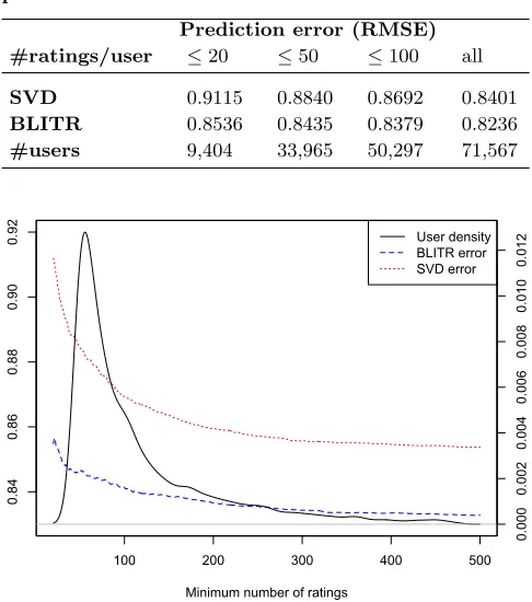
Table 3: Comparison of results over different user profile sizes.

Prediction error (RMSE) #ratings/user ≤20 ≤50 ≤100 all

SVD 0.9115 0.8840 0.8692 0.8401

BLITR 0.8536 0.8435 0.8379 0.8236

#users 9,404 33,965 50,297 71,567

100 200 300 400 500

0.84

0.86

0.88

0.90

0.92

Minimum number of ratings

Erro

r

density.default(x = errors$ratingCount[errors$ratingCount < 500 & errors$ratingCount > 19], freq = FALSE)

0.000

0.002

0.004

0.006

0.008

0.010

0.012

User density BLITR error SVD error

Figure 3: Prediction error and user count for vary-ing profile sizes

As discussed earlier, an important consideration for any

collaborative filtering algorithm is how well it does in the most difficult cases. This is generally users (or items) with a very small number of training ratings, for example the case of a new user or item. Analysing the data set we find that 13.4% of all users have 20 or fewer ratings and nearly half (47.5%) have 50 or fewer. We expect that these will be the users for whom the algorithms struggle the most to make accurate predictions for.

Table 3 shows how the performance of the best performing baseline and the best of the new models (SVD and BLITR) vary over different user profiles sizes. The results show that the BLITR model performs much better for smaller pro-files (relative to its performance over all users) than SVD. The SVD model’s performance decreases by 8.4% when deal-ing with small user profiles (20 or fewer ratdeal-ings) whereas BLITR’s performance only sees a very small decrease of 3.6%.

This result is perhaps illustrated more clearly in Figure 3, which shows the mean error over varying user profile sizes, for all users with a profile size smaller than or equal to the value on the x-axis. This is plotted for both SVD (dotted red line) and BLITR (dashed blue lines). The figure also shows on the right-hand y-axis the density of user counts over profile sizes (solid black line). We can see clearly that a large proportion of the users have a small number of ratings with very, very few having a large number. The maximum number of ratings for any user is 2876, 97% of users have fewer than 500 ratings and the minimum is 10 (this lower limit is imposed by the MovieLens web site). We can see from this plot that SVD’s error for users with small profiles is quite high and that it fairly rapidly decreases as the profile size increases. On the other hand LITR has much smaller error for users with small profiles and is able to produce much smaller errors than SVD over the whole range of profile sizes.

This is an important outcome as it demonstrates that our models are able to perform much better when data is par-ticularly sparse which is the most common case and are the situations for which we are most interested in improving performance. We speculate that this is a consequence of the Bayesian nature of the models; allowing them to cope better when there is little data available to base predictions on. It may also be because the LITR models are better at leverag-ing the limited information obtained from the small number of ratings that are available in these cases.

6.3

Variance of errors

0.5 1.0 1.5

0.0

0.5

1.0

1.5

2.0

density.default(x = errors$error[errors$error < 1.8])

Mean error over users

D

en

si

ty

BLITR

SVD

Figure 4: Density plot of mean error over all users

7.

CONCLUSIONS AND FUTURE WORK

In this work we have presented two Bayesian models for collaborative rating prediction based on clustering users and items into latent interests and latent topics simultaneously. We first introduced the concept of collaborative filtering and briefly discussed related work, including both memory and model-based methods. We motivated our work by outlining the benefits of model-based collaborative filtering systems and of the Bayesian approach to data modelling. The first model predicts a user-item rating by perturbing the mean rating across items and users by the weighted summation of interest and topic biases, where the weights are the proba-bility of the interest-topic pair given the particular user and item. The second model is an important and novel exten-sion of the first, including user and item specific biases in the prediction.

We describe an estimation procedure for this model which alternates between Gibbs sampling of the latent variables and an iterative fixed-point estimation of the additional bi-ases. We explain reasons why Gibbs sampling is both suit-able and necessary for this task, in particular that it allows new data to be easily, quickly and accurately folded into the existing model. We motivate the use of latent topics in the model due to their flexibility and the ease of interpreta-tion of results that they permit. We concede that the ideas of performing item recommendation using Bayesian proba-bilistic models and the inclusion of user and item biases are not in themselves novel. However the combination of these techniques via the interleaving of Gibbs sampling and fixed-point optimisation and the use of multinomial distributions for latent vectors for users and items and the byz matrix presents an important new contribution.

By experiment over a large, freely-available and commonly used data set of real item ratings we have shown that the models are extremely competitive, with the extended model significantly outperforming the most competitive baselines. Furthermore we investigated how well the strongest base-line and our best model performed in cases where the user profiles were very short (where the user had rated very few items). We found that our model is able to cope far better than the SVD baseline in these cases which is an important

result as such cases are both common and an area where improvement in performance is most useful. Lastly, analy-sis of the residual errors showed that BLITR’s errors had much smaller variance than those of SVD and as such is much less likely to generate extremely erroneous predictions which could frustrate and confuse users.

This work opens up many potential opportunities for fu-ture research by taking advantage of the modular strucfu-ture of the models to provide a framework for various extensions. Here we make a number of suggestions for future work:

• The models could be extended to include more infor-mation such as the time when each rating was made. It is likely that this would yield good improvements to the predictive power of the models as it did for partic-ipants in the Netflix prize.

• Improvements could be made to the fit of the models by estimating the variances of the various Gaussian mixture components separately, rather than using a fixed value. This may serve to improve the accuracy of predictions made.

• As noted earlier in the paper we calculate a point esti-mate for the user and item biases. The Bayesian ide-ology could be taken further by instead treating these as random variables with their own priors and calcu-lating a posterior for them in order to obtain a more principled, and potentially more accurate, estimate.

8.

REFERENCES

[1] G. Adomavicius and A. Tuzhilin. Toward the next generation of recommender systems: A survey of the state-of-the-art and possible extensions.Knowledge and Data Engineering, IEEE Transactions on, 17(6):734–749, 2005.

[2] D. Blei, A. Ng, and M. Jordan. Latent dirichlet allocation.Journal of Machine Learning Research, (3):993–1022, 2003.

[3] D. M. Blei and M. I. Jordan. Modeling annotated data. InSIGIR ’03: Proceedings of the 26th annual international ACM SIGIR conference on Research and development in informaion retrieval, pages 127–134, New York, NY, USA, 2003. ACM.

[4] J. S. Breese, D. Heckerman, and C. Kadie. Empirical analysis of predictive algorithms for collaborative filtering. InProceedings of the14th Annual Conference on Uncertainty in Artificial Intelligence (UAI98), pages 43–52, 1998.

[5] Wen Y. Chen, Jon C. Chu, Junyi Luan, Hongjie Bai, Yi Wang, and Edward Y. Chang. Collaborative filtering for orkut communities: discovery of user latent behavior. InProceedings of the 18th

international conference on World wide web, WWW ’09, pages 681–690, New York, NY, USA, 2009. ACM. [6] Andrew Gelman, John B. Carlin, Hal S. Stern, and

Donald B. Rubin.Bayesian Data Analysis. London: Chapman and Hall, 2004.

[7] D. Goldberg, D. Nichols, B. M. Oki, and D. Terry. Using collaborative filtering to weave an information tapestry.Communications of the ACM, 35:61–70, 1992.

[8] T. Griffiths and M. Steyvers. Finding scientific topics.

National Academy of Science, 2004.

[9] T. Hofmann. Unsupervised learning by probabilistic latent semantic analysis.Machine Learning, 42(1/2):177–196, 2001.

[10] T. Hofmann. Latent semantic models for collaborative filtering.ACM Trans. Inf. Syst., 22(1):89–115, January 2004.

[11] Yehuda Koren. Factorization meets the neighborhood: a multifaceted collaborative filtering model. InKDD ’08: Proceeding of the 14th ACM SIGKDD

international conference on Knowledge discovery and data mining, pages 426–434, New York, NY, USA, 2008. ACM.

[12] G. Linden, B. Smith, and J. York. Amazon.com recommendations: Item-to-item collaborative filtering.

IEEE Internet Computing Jan/Feb, 2003. [13] B. Marlin. Modeling user rating profiles for

collaborative filtering. InNIPS17, 2003.

[14] B. N. Miller, I. Albert, S. K. Lam, J. A. Konstan, and J. Riedl. Movielens unplugged: Experiences with an occasionally connected recommender system. In

Proceedings of ACM 2003 Conference on Intelligent User Interfaces (IUI’03), 2003.

[15] A. Paterek. Improving regularized singular value decomposition for collaborative filtering. In

KDDCup.07, 2007.

[16] A. F. M. Smith and G. O. Roberts. Bayesian

computation via the gibbs sampler and related markov chain monte-carlo methods (with discussion). In

Journal of the Royal Statistical Society, volume 55, pages 3–23, 1993.

[17] David H. Stern, Ralf Herbrich, and Thore Graepel. Matchbox: large scale online bayesian

recommendations. InProceedings of the 18th international conference on World wide web, WWW ’09, pages 111–120, New York, NY, USA, 2009. ACM. [18] Mark Steyvers, Padhraic Smyth, Michal R. Zvi, and

Thomas Griffiths. Probabilistic author-topic models for information discovery. InKDD ’04: Proceedings of the tenth ACM SIGKDD international conference on Knowledge discovery and data mining, pages 306–315, New York, NY, USA, 2004. ACM.