Reliability modeling and preventive maintenance of load-sharing systems with degrading components

Reliability modeling and preventive maintenance of

load-sharing systems with degrading components

Abstract

This paper presents certain new approaches to reliability modeling of systems subject to

shared loads. It is assumed that components in the system degrade continuously through additive

impact under load. Reliability assessment of such systems is often complicated by the fact that

both the arriving load and the failure of components influence the degradation of the surviving

components in a complex manner. The proposed approaches seek to ease this problem by first

deriving the time to prior failures and the arrival of random loads and then determining the

number of failed components. Two separate models capable of analyzing system reliability as

well as arriving at system maintenance and design decisions are proposed. The first considers

constant load and the other cumulative load. A numerical example is presented to illustrate the

effectiveness of the proposed models.

Keywords: load sharing system, continuous degradation, random load, reliability model, preventive maintenance

Notation

(

,

)

CR  P Maintenance cost rate

( )

i

F t cdf of the ith failure time

( )

T

F t cdf of the system failure time

( )

i

f t pdf of the ith failure time

H Failure threshold of a component

k

L Magnitude of the kth arrived load

( )

L t Total load magnitude on the system at time t

( )

l t Load magnitude of a component at time t

( )

( )

N t Number of failed components by time t

Nr Number of repetitions for Monte Carlo simulation n Number of components in the system

P Degradation threshold for preventive maintenance

( )

R t Reliability of the system at time t

( )

r t Reliability of a component at time t

S Length of a renewal cycle

T Time to system failure

i

T Time to the ith failure P

T Time to reach preventive maintenance threshold

j

t _{Arrival time of the jth load}

( )

X t Degradation amount of a component by time t

 Degradation rate

 Arrival rate of random loads  _{Initial degradation amount}

( )

 cdf of standard normal distribution



Periodical inspection interval

1.

Introduction

It is often assumed in reliability engineering that failures are independent, i.e., failure of a

component has little effect on failures of other components. However, many systems are load

sharing (all the components work together and share system load) in practice. The assumption of

independence is not valid in such a system. If a component fails the same workload has to be

shared by the surviving components, so each surviving component experiences an increased load

(Singh and Gupta, 2012). The increased load would probably induce a higher failure rate.

Load-sharing systems have been applied widely in industrial practice. For example, in a

distributed computer system, servers work together to finish the workload imposed on the system

certain load sharing rule (Yu et al., 2013); in a power grid, the total electricity demand is

distributed across several links in the net (Basu et al., 2012). More examples can be found in

(Kvam and Pena, 2005).

There exist numerous works in literature concerning load-sharing systems. However, most of

the studies have focused on statistical inference and parameter estimation of lifetime distributions

of load-sharing systems (Deshpande et al., 2010; Kim and Kvam, 2004; Singh et al., 2008;

Balakrishnan et al., 2011; Park, 2010; Park, 2013). In contrast, studies on the reliability analysis

of load-sharing systems are relatively rare. A reason is that the mechanism of how the load is

shared among components is too complex to permit a thorough analysis (Amari et al., 2008).

Another issue complicating the analysis is that load history affects the reliability of the system

within its lifetime.

In most of the literature concerning reliability analysis, it has been assumed for the sake of

simplicity that the lifetime of a component follows an exponential distribution (Shao and

Lamberson, 1991; Yun et al., 2012; Qi et al., 2014). However, the assumption of exponential

lifetime distribution is questionable in many practical contexts. The restrictive assumption of

exponential distribution has been relaxed in some studies (Singh and Gupta, 2012; Durham et al.,

1997; Liu, 1998; Ibnabdeljalil and Curtin, 1997; Amari and Bergman, 2008). Amari and Bergman

(2008) analyzed load-sharing systems with general lifetime distribution with Tampered Failure

Rate (TFR) model and Cumulative Exposure (CE) model. It was emphasized that an appropriate

model must be carefully chosen to account for the influence of load history, so as to extend the

results of the case of exponential distribution to the case of general distribution. Liu (1998)

investigated the reliability of k-out-of-n systems, where the lifetime distribution of the

components is arbitrary. Nonetheless, there is no closed-form solution and numerical methods

have to be used to compute the system reliability. Singh and Gupta (2012) analyzed system

reliability assuming Lindley lifetime distribution of components and estimated the parameters

a Weibull lifetime distribution and studied the failure mechanism of fibers under localized

load-sharing rule. Ibnabdeljalil and Curtin (1997) studied the reliability and strength of

fiber-reinforced composites under local load-sharing condition. The study demonstrated that the

ultimate strength decreases with the composite size and failure occurs by local accumulation of a

critical amount of damage.

An assumption implicit in the previous studies is that the components are static; the condition

of component is invariant and component failure is sudden and catastrophic. However, in many

real world applications, the working environment is usually dynamic and a change in

environment may lead to a change in the physics of failures. Many systems and components go

through a period of degradation and cease functioning when the degradation amount reaches a

critical threshold level. This type of failure is said to be ‘soft failure’ (Ye et al., 2012).

Singpurwalla (1995) pointed out that modelling failure using a stochastic-process approach

provides flexibility with respect to describing the failure-generating mechanisms. One advantage

of using degradation model is that the degradation level can be detected by inspection/monitoring

equipment and therefore the relationship between load and system failure can be more accurately

characterized. By taking advantage of the degradation model, we conduct reliability analysis and

maintenance policy for load-sharing systems in a continuous degradation context.

In traditional approaches for reliability analysis, proportional hazards models are established to

account for the effect of loads on component lifetime distribution (Liu, 1992; Amari and

Bergman, 2008). However, for a load-sharing system with continuously degrading components,

both the internal degradation process and the external loads have effects on system reliability.

The proportional hazards method is limited to a two-state system and cannot model the system

behavior with continuous degradation. A novel reliability model is required to address

load-sharing system with degrading components. Actually, in the work of Peng et al. (2010), the

authors developed a reliability model for system with multiple dependent competing failure

degradation and external shocks. In our study for load-sharing system, the cumulative shock

model is also used for the service of reliability modeling. While Peng et al. (2010) was focused

on reliability analysis for a single-component system, we proceed to integrate the cumulative

shock model into load-sharing context.

Preventive maintenance strategies for multi-component systems have been studied extensively

in the literature (Moghaddam and Usher, 2011; Liu et al., 2014; Wang and Pham, 2011; Wang et

al., 2014). Most maintenance policies currently in vogue for multi-component systems focus on

the economic dependence among components. To the best of our knowledge, few studies have

addressed the issue of preventive maintenance for load-sharing systems, although this is a very

common situation when a system does not fail completely after a component failure but the loads

on others go up.

In this paper, we construct reliability models for load-sharing systems subject to degrading

components so as to arrive at a preventive maintenance strategy. At first we obtain some

preliminary insights by modeling system reliability with constant load. Next we build a reliability

model assuming varying loads. Specifically we consider the scenario where the load is random

and has a cumulative impact on the system. Finally, we utilize the proposed reliability models to

arrive at preventive maintenance decisions.

The remainder of this paper is organized as follows. Section 2 presents the specifications of

the system including assumptions, system description and the load sharing rule. In section 3, we

construct two reliability models considering constant load and cumulative load separately. A

preventive maintenance model with inspection interval and preventive maintenance threshold

being optimized simultaneously is developed in Section 4. A numerical example is presented in

Section 5 to illustrate the effectiveness of the reliability models at arriving at maintenance

policies. Finally, Section 6 concludes the study and makes some suggestions for further work.

2.1 System description

The following assumptions have been adapted from (Peng et al., 2012; Harlow and Phoenix,

1978; Huang and Xu, 2010; Peng et al., 2010; Rafiee et al., 2014) in formulating the basic

reliability model presented in this paper.

1. All the components in the system are identical.

2. Each component is subject to continuous degradation. For a component, denote the

degradation amount over time t asX t( ; , )  , where  is a fixed parameter and  is a

random variable.

3. Load is equally distributed on each component.

4. Load imposed on a component has an additive impact on the degradation amount of the

component.

5. Each component is deemed to have failed when the degradation amount exceeds a critical

threshold H.

The system considered here is a parallel system consisting of n identical components.

Generally, the degradation process of each component could be in any form of a stochastic

process. Linear degradation is assumed (Peng et al., 2012), i.e., X t( )= + t, where the initial degradation amount  is a constant and the degradation rate  is a random variable, following a

normal distribution,



N(

 

_, _2). We assume that _ _, so that the probability of the

degradation level being negative can be neglected. A component is deemed to have failed if its

degradation amount X t( ) exceeds the threshold, H. The assumption of linear degradation is used

widely in systems such as micro-electro-mechanical systems (Peng et al., 2012; Peng et al., 2010)

and laser devices (Peng and Tseng, 2009).

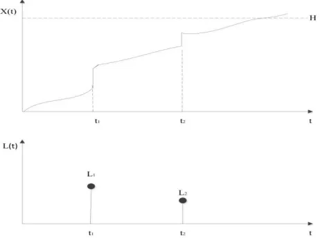
Assumption (4) states that the load has an additive impact on the degradation of a component,

i.e.,

( ) ( )

where ( )l t is the load imposed on the component. Fig. 1 shows the degradation process of a

component with the influence of loads. In the figure, loads arrive at time t₁ and t₂, causing an abrupt change in the degradation amount of the component. It should be noted that the system

load can either be a constant or a random variable. We will discuss the reliability model for

constant load and cumulative load separately in Section 3.

Fig.1: Degradation process of a component subject to loads

2.2 Load-sharing rule

Load-sharing rules determine how system load is distributed among components and how the

load on a surviving component changes when some components fail (Harlow and Phoenix, 1978).

Typically, load-sharing rules come in three kinds: equal load-sharing rule, local load-sharing rule,

and monotone load-sharing rule (Amari et al., 2008). An equal load-sharing rule indicates that the

total system load is equally distributed among all its components, a local load-sharing rule

implies that the load on a failed component is transferred to adjacent components, and a

monotone load-sharing rule indicates that the load on the surviving components is non-decreasing

when other components fail. In this paper, we focus on the equal load sharing rule, i.e.,

( ) ( )

( ) L t l t

n N t =

[image:7.612.208.439.204.376.2]

where ( )L t is the total system load over time t, N t( ) is the number of failed components by

time t. The method we use to analyze the reliability of a sharing system with equal

load-sharing rule can also be applied to system with other load-load-sharing rules.

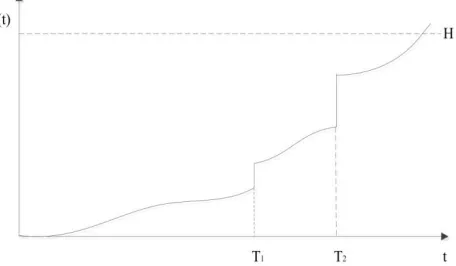
If a component fails, the load has to be shared by the remaining components, thus increasing

the degradation amount of the surviving components. Fig. 2 shows the degradation process of a

component under the influence of failures of other components. In the figure, failures occur at T1 andT2, inducing abrupt changes of the degradation amount in the surviving components.

Fig. 2: Degradation process of a component subject to inner failures

3. Reliability models for load-sharing system

As pointed out in the previous section, the degradation amount of a component is influenced

by its own degradation process, failure of other components and the imposed system load. The

difficulty of conducting a reliability analysis of such a system lies in the dependence between the

inner failures of components and the degradation amount of the surviving components, especially

when the system load is a random variable (Park, 2013; Huang and Xu, 2010). In this section, we

construct separate reliability models for load-sharing systems subject to constant load and

cumulative load. More specifically, we formulate a reliability model in Section 3.1 by considering

constant load and acquire several preliminary insights. The aim of section 3.1 is to study the

[image:8.612.212.440.280.413.2]

system under cumulative load to jointly analyze the effect of the system load and inner failures on

system reliability (see Section 3.2).

3.1 Reliability model concerning constant load

In this section, we assume that the load imposed on the system is constant. By using constant

load, we mean that only one load with magnitude L is imposed on the system, from the startup of

system operation. As the load is equally distributed to the components, the reliability of a

surviving component can be obtained as

1

0 1

0

( ) ( ( ) | ( ) ) ( ( ) )

( | ( ) ) ( ( ) )

n i n i

r t P X t H N t i P N t i

L

P t H N t i P N t i

n i

  −

= −

=

=  =  =

= + +  =  =

−





(3)

where P N t( ( )=i) denotes the probability that i components have failed by time t, and L is the constant load imposed on the system.

We assume that the degradation rate  follows a normal distribution,



N(

 

_, _2), so

( )

( | ( ) )

L

H t

L _{n i}

P t H N t i

n i t



    



 _{− + +} 

 ₋ 

+ +  = =  

− _{ }

 

(4)

Where ( ) is the cumulative distribution function (cdf) of a standard normally distributed variable. To compute ( ( )P N t =i), we utilize the cdf of the ith failure time and the (i+1)th failure time, F t_i( )and F_i+1( )t [14]. F t_i( )and F_i+1( )t can be obtained by the failure time history (Huang and Xu, 2010). The following theorem indicates how to compute P N t( ( )=i)with previous failure times.

1 1 1 1 1 1 1

1 1 1

( ( ) ) ( 1) ( ) ( 1)

( ) ( ) ( ) ( )

j j i

i i i

i _T

j j j T

j

T t t

i i i i i i i i i

T T T

P N t i n j f T dT n i

f T dT n i f T dT f T dT

+ − + − − − = + + + = = − +  − +   _ − − _  











(5)

where Tiis the time to the ith failure, T0=0, and fi( )is the probability density function (pdf) of the ith failure time, defined as

1 1 ( ) , ( ) 0, otherwise i i

i i i t T

i i

dF t

T T T

dt

f T = − +

 _{ }  =    (6)

Detailed proof is given in the Appendix.

We assume that each component follows a linear degradation process and the degradation rate



follows a normal distribution, so that

( )

1

( ) ( | ( ) 1)

i

L

H t

L _{n i}

F t P t H N t i

n i t

        _{− + +}   _{− +}  = + + ₋  = − =       (7)

For Ti−1 Ti Ti+1,

2 ( ) 1 ( ) i i i i i L H T H n i f T T T      _    _{− + +}     _{− +}  − =  _{ } _       (8) Let ( ) 1 ( ) i L H t n i t t       _{− + +}   _{− +}   =       (9)

Eq. (5) can now be rewritten as

( )

( )

( )

( )

( )

( )

( )

( )





1 1 1 1

1 1 1 1 1

( ( ) ; 1) ( 1) ( 1)

( )

i

j j j j j

i i i i i i i i i i

P N t i i n j T T n i

n i T T t T t T

− + − = + − + + −   =  = − + _ −  _ − +  − _ −   _{ } −   − _{ } −  _



(10)

( )

(

)

( )

( )

( )

( )

( )

( )

( )

( )

( )





1 0 1 1

1 1 1 1

1 1

1 1 1 1 1

( ) ( ( ) | ( ) ) ( ( ) )

( 1) ( 1)

( ) n i i n n

i j j j j

i j

i i i i i i i i i i

r t P X t H N t i P N t i

t t n j T T n i

n i T T t T t T

− = − − + + − = = + − + + − =  =  =   =  +   − + _ −  _ − +  − _ −   _{ } −   − _{ } −  _







(11)

Finally, the reliability of the system can be represented as

( )

( )

( )

( )

( )

( )

( )

( )





1 1 1 1 1 1 1 1

1 1 1 1 1

( ) ( ( ) ) ( ( ) )

( 1) ( 1)

( )

n i i

n

j j j j i j

i i i i i i i i i i

R t P N t n P N t i

n j T T n i

n i T T t T t T

− = − − + − = = + − + + − =  = =   = − + _ −  _ − +  − _ −   _{ } −   − _{ } −  _





(12)

3.2 Reliability model concerning cumulative load

For systems subject to varying loads, the arrival of a load is usually modeled as a renewal

process with an exponential, Weibull or Gamma distributed inter-arrival time (Peng et al., 2010);

the magnitude of a load is modeled as a continuous random variable. In this article, the following

specific assumptions are made to model the reliability of the load-sharing system under

cumulative load (Rafiee et al., 2014):

1. The load arrives according to a Poisson process with rate.

2. The magnitude of each arriving load is an independent and identically distributed (i.i.d.)

random variable, following a normal distribution, L_k N u( _L,_L2). It is assumed that

L L

  , so that the probability of negative loads can be neglected, i.e.,  −(  _L/ _L)0. The magnitude of the cumulative load can be expressed as

( )

1

, ( ) 0

( )

0, ( ) 0

M t k k

L if M t L t

if M t

=    =   ₌ 



₍₁₃₎

2

( ) ( _L, _L)

L t N ju j (14)

The reliability of a surviving component can then be expressed as

1

0 0

( ) ( ( ) | ( ) , ( ) ) ( ( ) | ( ) ) ( ( ) )

n i j

r t P X t H N t i M t j P N t i M t j P M t j

− 

= =

=



 = =  = =  = (15)

The probability that a component survives at time t given the number of failed components

and the number of arrived loads, P X t( ( )H N t| ( )=i M t, ( )= j), can then be expressed as

( )

( )

2 2 ( ) ( ( ) | ( ) , ) ( | ( ) , ) ( ) L L L L t

P X t H N t i M t j P t H N t i M t j

n i j H t n i j           = = = + +  = = −  _{− + +}   ₋  =   +       (16)

The number of the load arriving at time t is

( )

( ( ) )

!

t j

e t

P M t j

j

 _

−

= = (17)

The computation of the probability ( ( )P N t =i M t| ( )= j)is relatively complex since both the arrival time of load and the failure time of components influence the surviving components. Two

special cases are of particular interest.

Case 1: If the system is subject to no load by time t, it acts as a parallel system with

independent components, so that

( )

! ( ) ( )

( ( ) | 0) 1

!( )!

n i i

H t H t

n P N t i M t

i n i t t

          −   − +    − +  = = = __ _ _{ } − _ __

− _{     } (18)

Case 2: If no component fails by time t, we obtain

( )

( _{2 2 2} 1)

( ( ) 0 | )

n L L j H t n i

P N t M t j

t j          _{− + +}    _{− +}  = = =    +  _ _  _{ }   (19)

In general, when the system is subject to both cumulative load and inner failures,

( )

( ( ) | )

Theorem 2: For i1, j1, the probability that the number of failed components by time t is i, given the number of arrived loads can be obtained as

( )

1 1

1 1

1 1

1 1 1

1 1 1 1 , 1 1 1

1, 1 1 ,

1

,

( ( ) | ) ( 1) ( , )

( ) ( , ) ( , ) ( 1) ( , ) k l k l i l

i j i l

i j

j

i _{T t}

k l k l k l T t

k l

j

t t T t

i j i j i j i l i l i l

T t T t

l t t

i j i j i j T t

P N t i M t j n k g T t dT dt

n i g T t dT dt g T t dT dt

n i

g T t dT dt

+ + − − + + − − − − − − − = = − + + + = = = = − +   −       − +  −   

 



 

 

 

 (20) where 1 ( )

, _{2 2 2} 2

( 1) ( ) 1 ( , ) ( 1) j j L i t t i j i j

i i L j H T H n i

g T t e

T T j  _      _     − − − −  _{− + +}     _{− +}  ₋ =  _ _ + −        (21)

The proof is similar to that of Theorem 1.

Combining the above equations, the reliability of a component can be expressed as

( )

( )

( )

1 0 0

1 1

2 2 2

( ) ( ( ) | ( ) , ) ( ( ) | ) ( ) ( ) ( ) ( ) ( ) 1 n i j n n L t t L n

r t P X t H N t i M t j P N t i M t j P M t j

H t

H t _n

e e t

t

H t H t

n t      _            _{ }       −  = = + + − − =  = =  = =  =   _{− + +}    − +     = _ _ __ +    +        _{  }       − +  − + + _ _ __ −     



(

)

(

)

(

)

1 1 1 1 1 1 1 ( )

, 1 , 1

2 2 2

1 1 1 1

( ) (

1, 1, , 1 , 1

(22)

( )

( ) ( ) ( 1)

( ) ( ) ( ) ( ) ( ) l l j l t L j i n t t k l k k l k

i j k l

L

t t t t

i j i j i i j i i j i

e j

H t

n i _{T T e n i}

t j

n i t T e T T e

           + − − + − − − −  − − + − = = = = − − − − + + + −     _ _  _{ }    _{− + +}   ₋  +    −  − + +       −  −   −  





(

)

1 1 1 ) 1 ( )

, 1 , 1

( ) ! ( ) ( ) l j j t j l t t i j i i j i

e t

j

T T e

   − − − − = − − + −       _{−  − }   



where ,

2 2 2

, ( ) i j t

 can be interpreted as the cdf of failure time under i inner failures and j external loads.

Computation of the reliability in Eq. (22) requires the distribution of previous arrival times of

loads and failure time of components, which can be solved by iteration. The reliability of the

system can then be assessed as

1 1 1 1

1

1 1

1 1 1

1 1

, 1 1

1

1, 1 1 ,

1 1

( ) ( ( ) ) ( ( ) )= ( ( ) | ( ) ) ( ( ) )

( 1) ( , ) ( 1)

( ) ( , ) ( , )

k l

k l

i j

n n

i i j

j

i _{T t}

k l k l k l T t

k l n

t t

i j i j i j i l i l i T t

i j

R t P N t n P N t i P N t i M t j P M t j

n k g T t dT dt n i

n i g T t dT dt g T t dT d

+ + − − − − −  = = = − − = = −  + + + = = =  = = = = = − +  − + = _{− }





 

  

1 1

1 1 1 1 1 1 , ( ) ! ( , ) i l i l i j t j j _{T t}

l T t

l t t

i j i j i j T t

e t

t _j

g T t dT dt

 _ + + − − − − − − =       _{ } _{ } _{ } _{ } − _ _  

 

 

(23)

Although the developed reliability models are applied for parallel systems, they can be easily

extended to k-out-of-n systems. For a k-out-of-n: G system, system reliability can be expressed as

the probability that less than k components fail by time t. By using Eq. (12), we can have the

system reliability as R t( )=P N t( ( )k)=



k_i=1P N t( ( )=i).

4. Preventive Maintenance Policy

The system considered in this paper is highly integrated, e.g., a micro-electro-mechanical

system where repair or replacement of any individual component is particularly difficult or even

impossible (Peng et al., 2010). Thus, maintenance action has to be taken for the whole system. A

preventive maintenance model with periodic inspection is developed in this article. To evaluate

the performance of the maintenance policy, we adopt a long-run cost rate model where the

preventive maintenance threshold P and the periodic inspection interval  are the two decision

variables. The maintenance policy works as follows.

(1) The degradation level of the system exceeds the failure threshold, X i

( )

 H , then the system is replaced. Additional cost may be incurred during the downtime of the system.

(2) The degradation level of the system exceeds the threshold for preventive maintenance but

still works,H X i

( )

 P, then preventive maintenance is undertaken.

(3) The degradation level of the system does not exceed the threshold for preventive

maintenance, X i

( )

 P, then the system is left unchanged.

Remark: For a parallel system, the system fails when all the components have failed. As the

component in the system fails one by one, failure time of the system is equal to the failure time of

the last failed component and the degradation process of the system can be characterized as the

degradation process of the last failed component.

Both the preventive maintenance and replacement will bring the system back to the state of

“as good as new”. A renewal cycle is defined as the time interval between two consecutive

maintenance actions (preventive maintenance or replacement). A renewal process is executed

during succeeding cycles while further costs are incurred within each cycle. From the basic

renewal theory, the long-run cost rate CR can be computed by (Grall et al., 2002)

( )

 

 

lim

t

E TC C t

CR

t E S

→

= = (24)

where C t

( )

is the total maintenance cost incurred until time t, TC is the total cost within the

renewal cycle and S is the length of the renewal cycle.

The cost items include the inspection cost, the preventive maintenance cost, the replacement

cost, and the penalty cost due to the malfunction of the system (Peng et al., 2010). The expected

total maintenance cost of a renewal cycle can then be expressed as

 

 

_{ }

+

 

, if replacement takes place

, if preventive maintenance takes place

I I F R

I I P

C E N C E C

E TC

C E N C



 +

 = 

+

Synthesizing the above two maintenance actions at the end of a renewal cycle, Eq. (25) can

be rewritten as

E TC

 

=C E N_I

 

_I +

(

C E_F

 

 +C_R

)

E_1_{replacement}+C E_P _1_{preventive maintenance}_ (26) where 1_{{ }•} is the indicator function, C_I is the cost of each inspection, C_Fis the cost rate during system downtime, CR is the cost of replacement, CPis the cost of preventive maintenance, NIis number of inspections within a renewal cycle, and is the system downtime, i.e., time interval between system failure to the next inspection time.

The number of inspections within a renewal cycle is related to the system degradation level, in

a manner that X i

( )

  P X

(

(

i−1

)



)

. Let T_Pdenote the time when the system degradation level reaches P, so that the expected number of inspections within a renewal cycle, E N

 

I can be

expressed as

 

(

)

(

( )

(

(

)

)

)

( )

(

(

)

)

(

)

1 1

1

= 1

1

P P

I I

i i

T T

i

E N iP N i iP X i P X i

i F i F i

 

 

 

= =



=

= =   −

= − −







(27)

where

( )

P

T

F is the cdf of T_P, which can be computed in a way similar to the calculation of

( )

T

F .

The system downtime is the interval from the system failure time to the next inspection time,

that is,  = −i T. The expected system downtime is given as

 





(

)

(

)

( )

(

)

( )

(

( )

(

(

)

)

)

1

1 1

| = =

1

P P

I I

i i

T T T

i i

E E N i P N i

i t dF t F i F i





 

  



= 

− =

=

= − − −





(28)

 



( )



(

)

( )

(

( )

(

(

)

)

)

replacement 1

1

1 | = =

1

P P

I I

i

T T T

i

E P X i H N i P N i

F i F i F i

     =  =  _{ =}    = − −





(29)

Similarly, the expected value of preventive maintenance occurring at the end of a renewal

cycle is given by

 



( )



(

)

( )

( )

(

)

(

( )

(

(

)

)

)

preventive maintenance 1 1

1 | = =

1

P P P

I I

i

T T T T

i

E P H X i P N i P N i

F i F i F i F i

      =  =  _{ =}     = − − −





(30)

The length of a renewal cycle is determined by the number of inspections and the interval

between two inspections, that is, S=NI . Its expected value can be computed as

 



 (

)

( )

(

(

)

)

(

)

1 1 | = = 1 P P I I i T T i

E S P S N i P N i

i F i F i 

 =  = = = − −





(31)

Based on Eq. (24) to Eq. (31), the long-run maintenance cost rate, CR

(

,P

)

can be

obtained as

(

)

(

( )

(

(

)

)

)

(

( )

( )

)

(

( )

(

(

)

)

)

( )

(

(

)

)

(

)

(

)

( )

(

)

( )

(

( )

(

(

)

)

)

( )

(

( )

(

(

)

)

)

( )

(

(

)

)

(

)

1 1 1 1 1 1 1 1 1 , 1 1 1 1

P P P P P

P P

P P P P

P P

I T T P T T T T

i i

T T

i i

F _i T T T R T T T

i i

T T

i

C i F i F i C F i F i F i F i CR P

i F i F i

C i t dF t F i F i C F i F i F i

i F i F i

                       = =  =   − = =  = − − + − − − = − −  _{− − − +} _{ − −}     + − −















(32)

The optimal value of  and P can be obtained by solving

(

)

( )

,

, arg min ,

P

P CR P



  =  (33) Due to the interaction between and P and the complexity of CR

(

,P

)

, it is difficult to

5. Numerical Example

To investigate the reliability model and maintenance policy, we took a load-sharing redundant

microengine system as an example. A microengine often fails due to the visible wear on rubbing

surfaces between the gear and the pin joint (Peng et al., 2010). The wear is mainly caused by the

ageing degradation process. Meanwhile, external load shocks contribute to the debris between the

gear and the pin joint. Usually in a system, multiple microengines work together to perform tasks,

which can thus be modelled as a load-sharing system. We consider a system consisting of three

microengnes in a load-sharing parallel structure. Each microengine goes through a linear

degradation process individually, X t( )= + t, where the initial degradation amount  is a constant and the degradation rate  is a random variable, following a normal distribution,

2

( , )

N _{ }



 

. In the following section, we consider the case that the system is subject to

constant load L and cumulative load ( )L t respectively. The cumulative loads arrive according to a

homogeneous Poisson process with rate . The magnitude of each load arrived is assumed to be an i.i.d random variable, following a normal distribution, L_k N u( _L,_L2). A microengine fails

when the overall wear amount exceeds the threshold, H. Preventive maintenance is conducted

according to the observation of the visible wear amount. Table 1 summarizes the associated

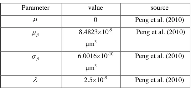
[image:18.612.154.459.562.703.2]

parameters for reliability analysis and maintenance policy.

Table 1: Summary of the parameters

Parameter value source

 _{0 Peng et al. (2010)}



 8.4823×10-9

μm3

Peng et al. (2010)



 6.0016×10-10

μm3

Peng et al. (2010)

L

 1×10-4 μm3 Peng et al. (2010)

L

 2×10-5 μm3 Peng et al. (2010)

H 0.00125μm3 _{Peng et al. (2010)}

L 0.0002 μm3 Peng et al. (2010)

CI $500 Assumption

CP $10,000 Assumption

CR $30,000 Assumption

CF $10 Assumption

5.1 Reliability analysis

We first analyzed the reliability of the system under constant load. The system reliability

function is given Eq. (12). However, it is very difficult to have the complete form of reliability

function due to the complexity of the expression. Hence, we turn to Monte Carlo simulation to get

the reliability function.

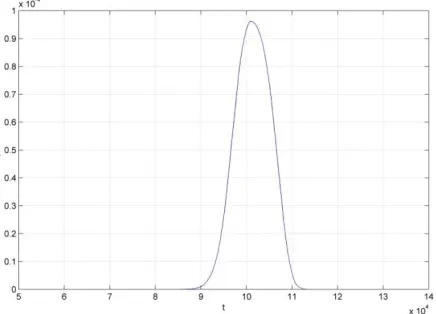
We compute system reliability with the number of repetitions Nr=10,000. Fig. 3 shows the

reliability variation noted within the time period_0.5 10 ,1.5 10 5  5_. Fig. 4 shows the pdf of failure time under constant load. The pdf was computed numerically using the equation

(

)

( ) ( ) ( ) /

T T T

f t = F t+  −t F t t, where t is the time increment. We can observe that the system reliability began to decrease at time 5

0.98 10

t=  and reached 0 at time 5

1.12 10

t=  . We believe that small variation in the degradation process accounts for the rapid decrease. We also

investigated the impact of failure threshold on system reliability and undertook a sensitivity

analysis of failure threshold (see Fig. 5). Note that the failure threshold had shifted from 0.00115

μm3

to 0.00135 μm3, which implies that higher failure threshold increases the reliability of the

system.

Also, to examine the effect of number of repetitions, we selected the system reliability at

several times and compare the results for various Nr. We selected the system reliability from

5

1 10

t=  to 5

1.1 10

4 showed the system reliability for various number of repetitions Nr. It is indicated that when 1,000

r

N  , the difference of system reliability is within 0.01, which implies the effectiveness of the Monte Carlo simulation method.

Fig. 3: Reliability of system under constant load

[image:20.612.212.435.178.335.2] [image:20.612.215.433.395.552.2]

[image:21.612.222.424.80.224.2]

Fig. 5: Sensitivity analysis of failure threshold

Table 2: reliability variation with number of repetitions t

Nr

30 32 34 36 38 40 42 44 46 48 50

100 0.990 0.980 0.950 0.940 0.860 0.720 0.60 0.470 0.300 0.150 0.030

500 0.998 0.984 0.97 0.926 0.852 0.748 0.61 0.442 0.268 0.118 0.042

1,000 0.99 0.976 0.953 0.916 0.847 0.738 0.593 0.429 0.264 0.129 0.049

5,000 0.989 0.978 0.961 0.923 0.847 0.739 0.596 0.437 0.272 0.136 0.059

10,000 0.992 0.978 0.951 0.919 0.845 0.740 0.603 0.436 0.270 0.138 0.053

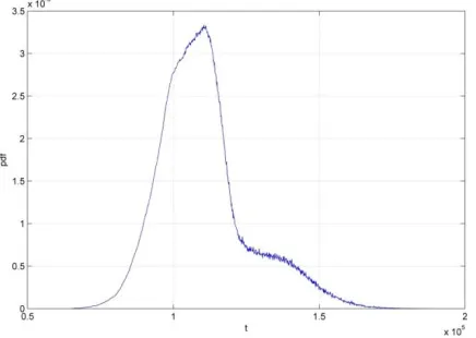
According to Eq. (23), we plotted the reliability of the system subject to cumulative load, as

shown in Fig. 6. We can observe that the reliability of the system started to descend at time

5

0.8 10

t=  and hit 0 at time t=1.7 10 5. Compared with the reliability variation with constant load, the system reliability with cumulative load possessed longer deteriorating duration. This is

due to the fact that the randomness of the arriving load adds more uncertainty to the degradation

process. For system subject to cumulative load, monitoring/inspection techniques play a more

significant role in reducing the uncertainty of the system. We also plotted the pdf of failure time

( )

T

f t in Fig. 7.

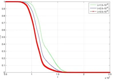
We are interested in the parameter of failure threshold H and load arrival rate, and make

[image:21.612.85.530.290.432.2]

larger threshold would lead to a higher reliability performance. In Fig. 9, when  increases from

5

1.5 10

_{= } −

to=3.5 10 −5, system reliability shifts to the left. This indicates that reliability

deteriorates faster when the system is subject to loads with higher arrival rates.

Fig. 6: Reliability of a system under cumulative load

[image:22.612.221.429.179.324.2] [image:22.612.214.432.382.537.2]

Fig. 8: Sensitivity analysis of failure threshold

Fig. 9: Sensitivity analysis of



5.2 Optimal preventive maintenance policy

The optimal values in Eq. (33) were determined using a numerical method. The cost

parameters are listed in Table 1. Table 3 shows the maintenance cost rate results CR

(

,P

)

as a

function of inspection interval and preventive maintenance threshold for a system subject to

constant load. Note that the minimum cost rate was 5.245 at

(



  =,P

)

(

10.5 10 ,7.7 10 4  −4

)

. For a system subject to cumulative load, we can obtain the minimum cost rate of 5.437, at

(

)

(

4 4

)

,P 11 10 ,5.7 10



_{  =  } −

. Table 4 shows the variation of maintenance cost rate CR

(

,P

)

as

[image:23.612.221.425.81.226.2] [image:23.612.225.423.284.428.2]

From Table 3 and Table 4, we can observe that the cost rate CR

(

,P

)

decreases with  before

 = , and increases afterwards. However, the effect of preventive maintenance threshold P is rather obscure. It can be concluded that the inspection interval



is the main contributor to the

[image:24.612.87.529.216.471.2]

variation of the cost rate.

Table 3: Maintenance cost rate with constant load vs P and





(104₎

P(10-4₎

8 8.5 9 9.5 10 10.5 11 11.5 12 12.5 13

7.5 6.831 6.609 6.165 5.784 5.435 5.261 5.414 5.619 5.797 5.962 6.128

7.7 6.831 6.666 6.213 5.749 5.435 5.245 5.417 5.613 5.799 5.960 6.118

7.9 6.847 6.703 6.250 5.808 5.456 5.264 5.408 5.619 5.800 5.962 6.121

8.1 6.837 6.768 6.313 5.858 5.448 5.253 5.420 5.621 5.811 5.962 6.122

8.3 6.842 6.798 6.439 5.900 5.501 5.258 5.412 5.615 5.793 5.967 6.127

8.5 6.843 6.878 6.490 5.977 5.534 5.275 5.418 5.621 5.799 5.962 6.121

8.7 6.853 6.897 6.608 6.043 5.564 5.280 5.417 5.619 5.807 5.970 6.117

8.9 6.843 6.919 6.650 6.152 5.680 5.305 5.427 5.608 5.798 5.966 6.124

9.1 6.842 6.957 6.802 6.223 5.698 5.326 5.444 5.641 5.794 5.970 6.124

9.3 6.847 6.986 6.835 6.353 5.756 5.366 5.460 5.623 5.792 5.964 6.122

9.5 6.846 6.994 6.902 6.449 5.784 5.417 5.483 5.625 5.808 5.973 6.118

Table 4: Maintenance cost rate with cumulative load vs P and





(104₎

P (10-4₎

8 8.5 9 9.5 10 10.5 11 11.5 12 12.5 13

5.5 6.511 6.194 5.838 5.602 5.510 5.504 5.475 5.613 5.752 5.874 6.078

5.7 6.509 6.116 5.888 5.587 5.480 5.455 5.437 5.628 5.762 5.965 6.008

5.9 6.479 6.154 5.823 5.616 5.538 5.472 5.521 5.548 5.771 5.944 6.088

6.1 6.564 6.144 5.846 5.599 5.518 5.464 5.534 5.623 5.742 5.899 6.062

6.3 6.485 6.167 5.871 5.636 5.517 5.447 5.529 5.644 5.785 5.900 6.025

6.5 6.448 6.154 5.869 5.624 5.488 5.475 5.486 5.638 5.717 5.911 6.086

[image:24.612.85.529.523.705.2]

6.9 6.375 6.132 5.844 5.682 5.495 5.495 5.539 5.610 5.762 5.843 6.119

7.1 6.340 5.881 6.802 5.590 5.507 5.507 5.499 5.634 5.727 5.910 6.012

7.3 6.431 5.814 6.835 5.624 5.496 5.496 5.540 5.642 5.758 5.890 6.119

7.5 6.332 5.836 6.902 5.642 5.523 5.523 5.511 5.585 5.786 5.860 6.076

6.

Conclusion

This paper has developed two reliability models for assessing the reliability of load-sharing

systems with continuously degrading components. The first has considered the case of constant

load and assessed the effect of failures of components on the surviving components. The second

has modeled systems subject to cumulative load and examined the influence of random load and

the influence of inner failures. Finally, the proposed models have been utilized to formulate

preventive maintenance policies for load-sharing system.

Future investigations can aim at relaxing some assumptions in this study. For example, this

study considers cumulative load model; future works can consider competing failure modes,

where the system may fail due to either soft failures (e.g., degradation) or catastrophic failures (e.g., shocks). In addition, this study conducts reliability analysis and maintenance policy for load-sharing systems in parallel structure. Extension to other complex structures (e.g., parallel-series, series-parallel bridge structure) is also of interest to investigate. Also, compared with equal

load-sharing rule used in this study, other load-sharing rules (e.g., local load-sharing rule or monotone load-sharing rule) may be more practical in some real applications. Load-sharing

systems with non-identical components can also be investigated.

Acknowledgement

The work described in this paper is supported by a grant from City University of Hong Kong

(Project No.9380058) and also by National Natural Science Foundation of China (No. 71371163).

References

Amari, S. V., and Bergman, R. (2008) Reliability analysis of k-out-of-n load-sharing systems.

Amari, S. V., Misra, K. B., and Pham, H. (2008) Tampered failure rate load-sharing systems:

status and perspectives. Handbook of Performability Engineering, Springer, London.

Balakrishnan, N., Beutner, E., and Kamps, U. (2011) Modeling parameters of a load-sharing

system through link functions in sequential order statistics models and associated

inference. IEEE Transactions on Reliability, 60(3), 605-611.

Basu, A. K., Bhattacharya, A., Chowdhury, S., and Chowdhury, S. P. (2012) Planned scheduling

for economic power sharing in a CHP-based micro-grid. IEEE Transactions on Power Systems,

27(1), 30-38.

Deshpande, J. V., Dewan, I., and Naik-Nimbalkar, U. V. (2010) A family of distributions to

model load sharing systems. Journal of Statistical Planning and Inference, 140(6), 1441-1451.

Durham, S. D., Lynch, J. D., Padgett, W. J., Horan, T. J., Owen, W. J., and Surles, J. (1997)

Localized load-sharing rules and Markov-Weibull fibers: a comparison of microcomposite

failure data with Monte Carlo simulations. Journal of Composite Materials, 31(18),

1856-1882.

Grall, A., Dieulle, L., Bérenguer, C., and Roussignol, M. (2002) Continuous-time

predictive-maintenance scheduling for a deteriorating system. IEEE Transactions on Reliability, 51(2),

141-150.

Harlow, D., and Phoenix, S. L. (1978) The chain-of-bundles probability model for the strength of

fibrous materials I: Analysis and conjectures. Journal of Composite Materials, 12, 195–214.

Huang, L., and Xu, Q. (2010) Lifetime reliability for load-sharing redundant systems with

arbitrary failure distributions. IEEE Transactions on Reliability, 59(2), 319-330.

Ibnabdeljalil, M., and Curtin, W. A. (1997) Strength and reliability of fiber-reinforced composites:

localized load-sharing and associated size effects. International Journal of Solids and

Structures, 34(21), 2649-2668.

Kim, H., and Kvam, P. H. (2004) Reliability estimation based on system data with an unknown

Kvam, P. H., and Pena, E. A. (2005) Estimating load-sharing properties in a dynamic reliability

system. Journal of the American Statistical Association, 100(469), 262-272.

Levitin, G., and Dai, Y. S. (2007) Service reliability and performance in grid system with star

topology. Reliability Engineering & System Safety, 92(1), 40-46.

Liu, B., Xu, Z., Xie, M., and Kuo, W. (2014) A value-based preventive maintenance policy for

multi-component system with continuously degrading components. Reliability Engineering &

System Safety, 132, 83-89.

Liu, H. (1998) Reliability of a load-sharing k-out-of-n: G system: non-iid components with

arbitrary distributions. IEEE Transactions on Reliability, 47(3), 279-284.

Moghaddam, K. S., and Usher, J. S. (2011) Preventive maintenance and replacement scheduling

for repairable and maintainable systems using dynamic programming. Computers & Industrial

Engineering, 60(4), 654-665.

Park, C. (2010) Parameter estimation for the reliability of load-sharing systems. IIE

Transactions, 42(10), 753-765.

Park, C. (2013) Parameter estimation from load-sharing system data using the expectation–

maximization algorithm. IIE Transactions, 45(2), 147-163.

Peng, C. Y., and Tseng, S. T. (2009) Mis-specification analysis of linear degradation

models. IEEE Transactions on Reliability, 58(3), 444-455.

Peng, H., Coit, D. W., and Feng, Q. (2012) Component reliability criticality or importance

measures for systems with degrading components. IEEE Transactions on Reliability, 61(1),

4-12.

Peng, H., Feng, Q., and Coit, D. W. (2010) Reliability and maintenance modeling for systems

subject to multiple dependent competing failure processes. IIE transactions, 43(1), 12-22.

Qi, X., Zhang, Z., Zuo, D., and Yang, X. (2014) Optimal maintenance policy for high reliability

load-sharing computer systems with k-out-of-n: G redundant structure. Applied Mathematics

Rafiee, K., Feng, Q., and Coit, D. W. (2014) Reliability modeling for dependent competing

failure processes with changing degradation rate. IIE Transactions, 46(5), 483-496.

Shao, J., and Lamberson, L. R. (1991) Modeling a shared-load k-out-of-n: G system. IEEE

Transactions on Reliability, 40(2), 205-209.

Singh, B., and Gupta, P. K. (2012) Load-sharing system model and its application to the real data

set. Mathematics and Computers in Simulation, 82(9), 1615-1629.

Singh, B., Sharma, K. K., and Kumar, A. (2008) A classical and Bayesian estimation of a

k-components load-sharing parallel system. Computational Statistics & Data Analysis, 52(12),

5175-5185.

Singpurwalla, N. D. (1995) Survival in dynamic environments. Statistical Science, 10(1), 86-103.

Wang, Y., and Pham, H. (2011) A multi-objective optimization of imperfect preventive

maintenance policy for dependent competing risk systems with hidden failure. IEEE

Transactions on Reliability, 60(4), 770-781.

Wang, W., Zhao, F., and Peng, R. (2014) A preventive maintenance model with a two-level

inspection policy based on a three-stage failure process. Reliability Engineering & System

Safety, 121, 207-220.

Ye, Z. S., Shen, Y., and Xie, M. (2012) Degradation-based burn-in with preventive maintenance.

European Journal of Operational Research, 221(2), 360-367.

Yu, H., Eberhard, P., Zhao, Y., and Wang, H. (2013) Sharing behavior of load transmission on

gear pair systems actuated by parallel arrangements of multiple pinions. Mechanism and

Machine Theory, 65, 58-70.

Yun, W. Y., Kim, G. R., and Yamamoto, H. (2012) Economic design of a load-sharing

consecutive k-out-of-n: G system. IIE Transactions, 44(1), 55-67.

Appendix

1 1

( ( ) ) ( ( ) ) ( ( ) 1)

( ) ( )

( ) ( )

i i

i i

P N t i P N t i P N t i

P T t P T t

F t F t

+ + = =  −  + =  −  = − (A1)

Note that the time to the ith failure, T_i is a random variable. The probability that a component fails in an infinitesimal interval dT_iat time T_i is given as

1 2 1

( | , ,..., ) ( )

e i i i i i

P t=T T T T₋ = f T dT (A2) Note that there are n− +i 1 surviving components in the system by time Ti−1 t Ti, then the probability that the ith failure occurs in an infinitesimal interval dTiat time Ti is

1 2 1

( i| , ,..., i ) ( 1) ( )i i i

P t=T T T T− = n− +i f T dT (A3)

Since F ti( )is related with the previous failure times, we can obtain the joint probability of

the ith failure time and the previous inner failure times as

1

1 2 1

1 2 1 1 1 2 2 2 1 1

1

1

( , , ,..., )

( | , ,..., ) ( | , ,..., ) ... ( | ) ( )

( 1) ( ) ( 1) ( )

i

i i

i i i i

i t

i i i j j j

T

j

P T t T T T

P T t T T T P t T T T T P t T T P t T

n i f T dT n j f T dT

− − − − − − =  =   =   =  = =

_

− + 



− + (A4)

F ti( )can be viewed as the marginal distribution of P T( it T T, ,1 2,...,Ti−1) , and can be obtained as

1 1

1

1 1

1 2 1 1

1 1

1

( ) ( ; , ,..., )

( 1) ( ) ( 1) ( )

( 1) ( ) ( 1) ( )

i j

j

i j

i i i

i

t t

i i i j j j

T T

j i

t T

i i i j j j

T T

j

F t P T t T T T

n i f T dT n j f T dT

n i f T dT n j f T dT

− − + − − − − = − = =  = − +  − + = − +  − +













(A5)

The second item is due to T1T2 ... Ti−1Ti, and the third item is due to the definition of

( )

i i

(

)

1 1 1

1 1

1 1

1

1 1 1

( ( ) ) ( ) ( )

( 1) ( ) ( 1)

( ) ( ) ( ) ( )

j j i

i i i

i i

i _T

j j j T

j

T t t

i i i i i i i i

T T T

P N t i F t F t

n j f T dT n i

f T dT n i f T dT f T dT

+

−

+

− −

+ −

=

+ + +

= = −

= − +  − + 

− −











(A6)