Hamming Distance Spectrum of DAC Codes for
Equiprobable Binary Sources
Yong Fang,
Member, IEEE, Vladimir Stankovic,
Senior Member, IEEE, Samuel Cheng,
Member, IEEE, and
En-hui Yang,
Fellow, IEEE
Abstract—Distributed Arithmetic Coding (DAC) is an effective technique for implementing Slepian-Wolf coding (SWC). It has been shown that a DAC code partitions source space into unequal-size codebooks, so that the overall performance of DAC codes depends on the cardinality and structure of these codebooks. The problem of DAC codebook cardinality has been solved by the so-called Codebook Cardinality Spectrum (CCS). This paper extends the previous work on CCS by studying the problem of DAC codebook structure. We define Hamming Distance Spectrum (HDS) to describe DAC codebook structure and propose a mathematical method to calculate the HDS of DAC codes. The theoretical analyses are verified by experimental results.
Index Terms—Distributed source coding, Slepian-Wolf coding, distributed arithmetic coding, Hamming distance spectrum, code-book cardinality spectrum.
I. INTRODUCTION
A
RITHMETIC coding (AC) [1] is an effective method for data compression that works by mapping each source sequence onto a half-open interval [l, h), where0≤l < h < 1. Though the principle of AC codes is rather simple, a major technical problem when putting AC codec into practice is that one has to use infinite-precision real numbers to represent land h, which is impossible for a digital circuit. Fortunately, there is a canonical implementation in [2] that represents l
andh with finite-precision integers and utilizes some scaling rules to solve the problems of renormalizationandunderflow
that are caused by finite-precision operations. An alternative solution to the complexity and precision problems in the AC codec is to use quasi-AC(QAC) codes, which can be seen as a reduced-precision version of AC codes [3].
As other variable-length codes, AC codes suffer from error propagation when the bitstream is conveyed over noisy chan-nels. This problem can be solved by reserving a forbidden interval in[0,1)for error detection [4] and runningmaximum a posteriori (MAP) decoding for error correction [5]. For
This work was supported by the National Science Foundation of China (grant nos. 61271280 and 61377011), the Program for New Century Excel-lent TaExcel-lents in University of China (grant no. NCET-13-0481), Provincial Foundation for Youth Nova of Science and Technology of Shaanxi, China (grant no. 2014KJXX-41), and the Fundamental Research Fund for the Central Universities of China (grant nos. 2014YQ001 and QN2013086).
Y. Fang is with the College of Information Engineering, Northwest A&F University, Yangling, Shaanxi 712100, China (email: [email protected]). V. Stankovic is with the Department of Electronic and Electrical Engineering, University of Strathclyde, Glasgow, UK (email: [email protected]). S. Cheng is with the School of Electrical and Computer Engineering, University of Oklahoma, Tulsa, OK (email: [email protected]). E.-H. Yang is with the Department of Electrical and Computer Engineering, University of Waterloo, Waterloo, ON N2L 3G1, Canada (email: [email protected]). The corresponding author is Y. Fang.
QAC codes, state models can be defined and used in a straightforward manner for MAP or soft decoding [6]. Such solutions are known as joint source-channel AC (JSCAC). Forbidden interval reservation is not the only solution to this problem,e.g., [7] achieves the same goal by inserting segment markers at fixed positions of bitstreams. Besides hard markers, the soft synchronization mechanism is also a powerful option for the JSCAC which allows controlling the trade-off between redundancy and resilience [8]. To predict and evaluate the effectiveness of the JSCAC, [9] provides an analytical tool to derive the distance spectrum of the JSCAC and proposes an algorithm to compute the free distance of the JSCAC.
Recently, AC codes also find their application to loss-less distributed source coding(DSC), orSlepian-Wolf coding
(SWC) [10], which has traditionally been implemented with channel codes, e.g., turbo codes [11] andlow-density parity-check(LDPC) codes [12], [13], [14]. Such solutions are known as distributed AC(DAC) codes. In fact, DAC codes are dual codes of JSCAC codes, so they can be realized by either interval overlapping [15], [16], [17] or bitstream puncturing [18], [19], [20]. Naturally, DAC codes can be combined with JSCAC codes to obtain the so-calleddistributed JSCAC
(DJSCAC) codes, which allow the coexistence of overlapped and forbidden intervals to realize data compression and error correction simultaneously [21].
Since the emergence of DAC codes, a lot of work has been done to verify the coding efficiency of DAC codes [16]. An important finding is that the residual errors of DAC codes cannot be removed by increasing code rate and/or length [16]. Thus, it is better to quantitatively measure thecoding efficiency
of DAC codes in terms offrame-error-rate(FER) or symbol-error-rate (SER) at a given code rate. Moreover, it is shown that at least for short code length, DAC codes outperform LDPC-based SWC codes with acceptabledecoder complexity
[16].
However, the above results are heuristic and lack strict theoretical analyses. To obtain an illuminating insight into the coding efficiency anddecoder complexity of DAC codes, the concept of spectrum was introduced, and the following findings were reported in [22], [23], [24]:
length goes to infinity, and hence the per-symbol rate loss will vanish as code length increases [24].
• DAC spectrum will become uniformly distributed as the decoding proceeds, which implies that 1-away (in Hamming distance) codewords in each codebook cannot be removed by increasing code length [24]. Further, a loose lower bound of decoding error probability is given as(2−2R), whereis the crossover probability between source andside information(SI), andRis code rate [24]. • Two techniques can be used to improve the coding efficiency of DAC codes [24]. First, the permutation
technique can remove those closely-packed (in Ham-ming distance) codewords in each codebook. Second, the
weighted branchingtechnique can reduce the mis-pruning risk of proper paths during the decoding.
Besides the above advances, the authors of [25] also noticed the existence of 1-away (in Hamming distance) codewords in each DAC codebook and proposed the distributed block arithmetic coding (DBAC) to solve this problem.
In summary,the problem of deducing DAC codebook cardi-nality has been solved, but we still know very little about DAC codebook structure. The only thing we know about the latter problem is that 1-away (in Hamming distance) codewords in each DAC codebook almost always exist [24]. Obviously, to analyze the coding efficiency of DAC codes, more knowledge about DAC codebook structure is necessary. Motivated by this problem, this paper introduces the concept of Hamming dis-tance spectrum(HDS), which is essentially proportional to the average number ofd-away (in Hamming distance) codeword-pairs inside each DAC codebook. We denote the HDS by
ψn,R(d), a function with respect to (w.r.t.) inter-codeword Hamming distance d ∈ {0,· · ·, n} that is parameterized by code lengthnand rateR, and propose a mathematical method to calculate ψn,R(d). Equipped with the HDS, it may be possible to calculate the FER and SER of DAC codes. Notice that to distinguish from the HDS, the spectrum defined in [22], [23], [24] will be formally referred to ascodebook cardinality spectrum(CCS).
The rest of this paper is arranged as follows. Section II describes the encoding procedure of DAC codes. Section III briefly reviews the previous work on the CCS. Section IV defines the HDS for DAC codes and gives an example to illustrate how to calculate it by exhaustive enumeration. Sec-tion V develops a mathematical method to calculate ψn,R(1), which is then generalized to ψn,R(d) for d≥2 in Sect. VI. Two implementation issues during calculating ψn,R(d), i.e., complexity and convergency, are discussed in Sects. VII and VIII, respectively. Experimental results are presented in Sect. IX to verify the correctness of the proposed method. Finally, Sect. X concludes this paper.
Source Model Following [22], [23], [24], this paper restricts the research scope to equiprobable binary sources. The reason is that the tackled issue is difficult, thus we have to begin with the simplest but non-trivial source model to simplify the analysis and make many hard problems tractable. Note that, the concepts proposed in this paper (and previous work [22], [23], [24]) cannot easily be extended to nonuniform
sources, because in contrast to uniform sources, for nonuni-formsources, the DAC behaves like asourcecode rather than achannelcode, making it very difficult to build the concepts of codebook and space partitioning.
Notation This paper will adopt the notations defined in [26], which are also used in [24]. We use X to denote a random variable andf(X)to denote a function ofX. Correspondingly, we use x ∈ X to denote a realization of X, where X is the alphabet of X, andf(x) to denote a function of x. We useXn
,(X0,· · ·, Xn−1)to denote the tuple of n random
variables and xn
,(x0,· · ·, xn−1)to denote a realization of Xn. We use0n to denote the tuple ofnconsecutive0s, while the meaning of 1n is similar. We define [i: j]
,{i,· · ·, j}
and (i : j) , {(i+ 1),· · ·,(j−1)}, while the meanings of [i : j) and (i : j] are similar. Further, we define q[i:j)
,
(qi,
· · ·, qj−1)and the meanings ofq[i:j],q(i:j), andq(i:j] are
similar. For brevity, the crossover probability between source and SI is abbreviated to source-SI crossover probability and denoted by . Moreover, we use q to denote the length of enlarged intervals(the same as [22] and [23], while different from [24]). The operation of | · | may denote the absolute value of a number, thecardinality of a set, or thelength of an interval, depending on the operand. The dot product ofxnand
ynis denoted by
hxn, yn
i, and the Hamming distance between
xnandynis denoted byd
H(xn, yn). We use{(l, h] + ∆}and
{ξ(l, h]} to denote the interval shifting and interval scaling
operations, respectively,i.e.,
(
{(l, h] + ∆},(l+ ∆, h+ ∆]
{ξ(l, h]},(ξl, ξh] . (1)
The clip functionmax(0,·)is abbreviated to(·)+,i.e.,( ·)+
,
max(0,·).
II. REVIEW OFDAC ENCODING
Let Yn be a tuple of n independent and uniformly-distributed (i.u.d.) binary random variables with Yi ∼p(y) =
0.5, where y ∈ B , {0,1} and i ∈ [0 : n). Let Xn
be another tuple of n i.u.d. binary random variables with
Xi|{Yi =y} ∼ p(x|y) for x ∈ B. The correlation between XnandYn is modeled as a virtualbinary symmetric channel (BSC) with crossover probability p(0|1) = p(1|0) = . According to the Slepian-Wolf theorem [10], if only Yn is available at the decoder, lossless recovery of Xn will be possible at ratesR≥H(X|Y) =Hb()bits per symbol(bps), where Hb(·) denotes the binary entropy function (BEF), no matter whetherYn is available at the encoder or not.
To compress Xn, the rate-R, where 0 < R < 1, DAC encoder iteratively maps source symbols onto partially-overlapped intervals [0, q) and [(1−q),1), where q , 2−R [15], [16]. Let[Li, Hi)be the interval after coding Xi. It is easy to show that [L0, H0) = [0,1) and (Hi−Li) = qi =
2−iR [24]. Therefore, we only need to trace eitherL i orHi. It is usually more convenient to trace Li. As shown in [24],
Li=l(Xi), where
Since the length of the final interval after coding Xn is always qn, it can be uniquely identified by
d−log2qne = dnRebits. To obtain the bitstream ofXn, we scaleL
n to get
S ,2dnReL
n. It is easy to see S =s(Xn), 2dnRel(Xn). The final interval [Ln, Ln+qn)is now mapped onto[S, S+
2dnRe−nR), which will be referred to asscaled final interval. An important problem is: What is the range of S? This prob-lem can be solved by considering the following two extreme cases: If Xn = 0n, then[L
n, Hn) = [0, qn); and ifXn= 1n, then[Ln, Hn) = [(1−qn),1). Hence,Ln∈[0,(1−qn)]and furtherS ∈[0,(2dnRe−2dnRe−nR)]. Then we calculatedSe. Because (dnRe −nR) ∈[0,1), we have 2dnRe−nR ∈[1,2) and further d2dnRe−2dnRe−nRe = (2dnRe −1). Therefore,
dSe ∈[0 : 2dnRe), implying that dSecan be binarized into a string ofdnRebits, which is just the DAC bitstream ofXn.
Length of Scaled Final Interval For simplicity, we will no longer consider the case dnRe > nR in the following. The reason is: IfdnRe> nR, we can always re-encodeXn at rate
R0=dnRe/n, which will produce a bitstream with exactly the same length. Therefore, in the rest of this paper, S=q−nL
n and
s(Xn) =q−nl(Xn) = (1−q)hq[0:n)−n, Xni. (3)
It is easy to know S ∈ [0,(2nR−1)] anddSe ∈ [0 : 2nR). The scaled final interval after codingXnis always[S, S+ 1),
i.e., the length of the scaled final interval is always1.
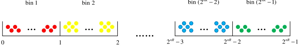
Illustration of DAC Encoding An illustration to better un-derstand DAC encoding is shown in Fig. 1. As shown in Fig. 1, if we take each codeword xn ∈
Bn as aball, DAC encoding
is equivalent to putting 2n balls into 2nR bins according to
s(xn). The rule is: Ifs(xn) = 0,xn is put into the0-th bin; otherwise ifs(xn)∈((m−1), m], wherem∈[1 : 2nR),xn
is put into the m-th bin (cf. Fig. 1).
III. REVIEW ONCODEBOOKCARDINALITYSPECTRUM
In this section, we briefly review the main results on CCS [22], [23], [24]. As shown in [24], a (2nR, n) binary DAC code is defined as
• an encoder m:Bn →[0 : 2nR) that assigns indexm∈
[0 : 2nR)to each source sequence xn
∈Bn, and
• a decoder xˆn : [0 : 2nR) → Bn∪ {e} that assigns an estimate xˆn
∈ Bn or an error message e to each index m∈[0 : 2nR).
The DAC encoding is in fact a many-to-one nonlinear mapping
Bn →[0 : 2nR), which unequally partitions source space Bn
into 2nR codebooks. Let Cm, where m ∈ [0 : 2nR), be the
m-th codebook. Ifxn∈ Cm, thends(xn)e=m and
s(xn)∈((m−1), m]∩[0,(2nR−1)]. (4)
Especially, if xn∈ C
0,s(xn)≡0; otherwise,s(xn)∈((m− 1), m]. Sincel(xn) =qns(xn),
l(xn)∈((m−1)qn, mqn]∩[0,(1−qn)]. (5)
Especially, if xn ∈ C
0, l(xn)≡0; otherwise, l(xn)∈((m− 1)qn, mqn].
An important property of DAC codebooks is cardinality, which is determined in [22], [23], [24] by defining the so-calledinitial spectrum.
Initial Spectrum Let X∞ , (X0, X1,· · ·) and q[0:∞) , (q0, q1,· · ·). BothL∞andH∞will converge to the following continuous random variable
U0,(1−q)hq[0:∞), X∞i, (6)
whose probability density function (pdf) f0(u) is called the
initial spectrum[22], [23], [24].
According to the definition off0(u), form∈[1 : 2nR), the cardinality ofCmis proportional to the integral off0(u)over
((m−1)qn, mqn]in the asymptotic sense, i.e., asn
→ ∞,
|Cm| →2n
Z mqn (m−1)qn
f0(u)du. (7)
Fornsufficiently large, the interval((m−1)qn, mqn]will be so short thatf0(u)almost holds constant in((m−1)qn, mqn]. Thus |Cm| → f0(mqn)2n(1−R) as n → ∞, i.e., |Cm| is proportional to f0(mqn) in the asymptotic sense. For this reason, we will call f0(u) the codebook cardinality spec-trum (CCS) from now on. For equiprobable binary sources,
Pr{Xn=xn} ≡2−nfor allxn∈
Bn. Thus, for allxn∈ Cm,
Pr{Xn=xn|Xn ∈ C
m} ≡1/|Cm|, and for allm∈[0 : 2nR),
Pr{ds(Xn)e=m}=|C m|2−n.
The0-th Codebook Becauseds(xn)e= 0only if xn = 0n,
C0 has one and only one codeword 0n in any case, and its
cardinality is always1,i.e.,|C0| ≡1.
Conditional CCS The pdf of U0givenXj =b∈Bis called
the conditional CCSgivenXj =b, and denoted byf0,j(u|b) [27].
Though DAC codebookcardinality has been well studied, very little about DAC codebookstructureis known up to now. The only thing we know is that for a (2nR, n) binary DAC code, as n → ∞, the proportion of twin leaf nodes in the decoding tree will tend to(2−2R). Thus, the decoding error probability is lower bounded by (2−2R), where is the source-SI crossover probability [24].
IV. HAMMINGDISTANCESPECTRUM
Just as channel codes, it is rather intuitive that another very important property of DAC codes is how far (in Hamming distance) the codewords in each codebook keep away from each other. Therefore, we will below define the Hamming distance spectrum (HDS) to measure quantitatively the dis-tribution of inter-codeword Hamming distances within each DAC codebook, which will be helpful for understanding DAC codebook structure.
A. Definition of Hamming Distance Spectrum
Codeword HDS The HDS w.r.t. codewordXn is defined as
kd(Xn),
n
˜
Xn :ds(Xn)e=ds( ˜Xn)eanddH(Xn,X˜n) =d
o .
0 1 2 2nR 3
− 2 2
nR
− 2 1
nR
−
bin 1 bin 2 bin (2nR 2)
− bin (2 1)
nR
−
……
[image:4.612.54.563.61.146.2]…
…
…
…
Fig. 1. Explanation of DAC encoding withball binning. The horizontal axis iss(xn).
In plain words, kd(Xn) is the number of codewords X˜n in codebook ds(Xn)e = m that are d-away (in Hamming distance) from Xn. It is easy to see d ∈ [0 : n] and
0 ≤ kd(Xn) ≤ nd. If we define k0(Xn) = 1, then
Pn
d=0kd(Xn) =|Cm|.
Codebook HDS The HDS of the m-th codebook is defined as
φm(d),E[kd(Xn)|Xn ∈ Cm]. (9)
Code HDS The HDS of the(2nR, n)DAC code is defined as
ψn,R(d),E[kd(Xn)]. (10)
It is easy to see that φm(d)is proportional to the number of d-away codeword-pairs within the m-th codebook and similarly, ψn,R(d) is proportional to the average number of
d-away codeword-pairswithin all codebooks of the (2nR, n) DAC code.
Asymptotic Code HDS The asymptotic HDS of the rate-R
DAC code is defined as
λR(d), lim
n→∞ψn,R(d). (11)
B. Calculating HDS by Exhaustive Enumeration
In practice, ψn,R(d) can be calculated by exhaustive enu-meration. Let us first considerφm(d). For equiprobable binary sources,
φm(d) =
X
xn∈C m
Pr{Xn=xn
|Xn
∈ Cm}kd(xn)
= (1/|Cm|)
X
xn∈C m
kd(xn), (12)
wherekd(xn)is a realization ofkd(Xn)[23]. Further, we can obtain
ψn,R(d) =
2nR−1
X
m=0
Pr{ds(Xn)e=m}φm(d)
= 2−n 2nR−1
X
m=0 X
xn∈Cm
kd(xn). (13)
Convexity of Sum-of-HDS Since Pn
d=0kd(xn) ≡ |Cm| for all xn
∈ Cm, we have [24] n
X
d=0
ψn,R(d) = 2−n
2nR−1
X
m=0 |Cm|2
→ 2n(1−R) Z 1
0
f02(u)du, (14)
as n→ ∞. Hence,
Γn ,
Pn
d=0ψn,R(d) 2n(1−R) →
Z 1
0
f02(u)du≥1. (15)
After expansion, we haveΓn=Qn−i=01γi, whereγiis the
level-iexpansion factor that is defined as the ratio of the number of level-(i+1)nodes to that of level-inodes in the DAC decoding tree [23]. Apparently,Γ∞is a nonnegative and convex function inf0(u), which takes the minumum value1only whenf0(u)
is uniform over[0,1). Similarly, we have
n
X
d=0
ψn,R(d)≥2n(1−R) (16)
and the equality holds only if |Cm| ≡ 2n(1−R), i.e., source spaceBn is equally partitioned into2nR codebooks of
cardi-nality2n(1−R).
C. Example of Hamming Distance Spectrum
To illustrate the concept of HDS, we give an example to show how to calculate ψn,R(d) for n = 4 and R = 0.5. The source space Bn contains 2n = 16 codewords and is
partitioned into 2nR = 4 codebooks. We list all codewords of the source space in Tab. I. For each codeword xn, s(xn) (the lower bound of the scaled final interval) and m (the corresponding codebook index) are included in Tab. I, where different codebooks are marked with different colors for clar-ity. We also plot the positions ofs(xn)for all codewords xn
in Fig. 2. It can be seen that|C0|= 1,|C1|= 4,|C2|= 7, and |C3|= 4. We list the HDS of each codeword in Tab. I. After
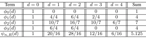
a simple calculation, we obtain the HDS of each codebook and the code HDS, as shown in Tab. II. It is easy to verify
Γn = 5.125/4>1.
V. MATHEMATICALCALCULATION OFψn,R(1) For a largen, it is difficult to calculate code HDS ψn,R(d) through exhaustive enumeration in Subsect. IV-C because it needs the HDS kd(xn) of all 2n codewords. To get around it, we propose below a mathematical method that is able to obtain ψn,R(d) directly in the absence of kd(xn). The procedure of the proposed method is still very time-consuming for large d. Nevertheless, this is usually enough in practice because the decoding failure of DAC codes is caused mainly by closely-packed (in Hamming distance) codewords within each codebook. For clarity, we first use the simplest case
0
1
2
3
0001
0100
0010
0011
1000
0101
0110
1001
1010
0111
1100
1011
1101
1110
1111
0000
[image:5.612.55.298.485.549.2](
n)
s
x
Fig. 2. Example for illustrating the mapping ofxnands(xn), wheren= 4andR= 0.5. Each node at the horizontal axis denotes the position ofs(xn)
corresponding to codewordxn. Different codebooks are marked with different colors.
TABLE I
EXAMPLE OFCODEWORDHDS
xn s(xn) m k
0(xn) k1(xn) k2(xn) k3(xn) k4(xn)
0000 0.0000 0 1 0 0 0 0
0001 0.4142 1 1 1 2 0 0
0010 0.5858 1 1 1 2 0 0
0011 1.0000 1 1 2 0 1 0
0100 0.8284 1 1 0 2 1 0
0101 1.2426 2 1 1 3 1 1
0110 1.4142 2 1 1 3 1 1
0111 1.8284 2 1 2 0 3 1
1000 1.1716 2 1 3 0 2 1
1001 1.5858 2 1 1 3 1 1
1010 1.7574 2 1 1 3 1 1
1011 2.1716 3 1 1 2 0 0
1100 2.0000 2 1 1 4 1 0
1101 2.4142 3 1 1 2 0 0
1110 2.5858 3 1 1 2 0 0
1111 3.0000 3 1 3 0 0 0
Sum — — 16 20 28 12 6
TABLE II
EXAMPLE OFCODEBOOKHDSANDCODEHDS
Term d= 0 d= 1 d= 2 d= 3 d= 4 Sum
φ0(d) 1 0 0 0 0 1
φ1(d) 1 4/4 6/4 2/4 0 4
φ2(d) 1 10/7 16/7 10/7 6/7 7
φ3(d) 1 6/4 6/4 0 0 4
ψn,R(d) 1 20/16 28/16 12/16 6/16 5.125
this section and then extend it to the general case d≥ 2 in the next section. The core idea of our proposed method is to expandψn,R(d)as the sum of multiple tractable terms (called
atoms below). To achieve this goal, we define the following important concept.
XOR Pattern We refer to Zn = (Xn
⊕X˜n) as the XOR
pattern between Xn and X˜n, where Xn and X˜n are two binary vectors.
A. Expansion of ψn,R(1) as Sum-of-Atoms
Given dH(Xn,X˜n) = 1, there are n1=ndifferent XOR patterns between Xn and X˜n, which must take the form of
zn(j)
,(0j,1,0n−j−1), where j ∈[0 :n). Let z
i(j) be the
i-th element of zn(j), then z
j(j) = 1 and zi(j) = 0 for all
otheri6=j. We define
k(1j)(Xn),
n
˜
Xn:ds( ˜Xn)e=ds(Xn)eand (Xn⊕X˜n) =zn(j)o .
(17)
In plain words,k1(j)(Xn)is the number of codewordsX˜n in
codebook ds(Xn)e = m that satisfy (Xn ⊕X˜n) = zn(j). It is easy to seek1(j)(Xn) = 0 or 1, and
Pn−1
j=0k (j)
1 (Xn) = k1(Xn), where k
d(Xn) is the codeword HDS of Xn (see Subsect. IV-A). With the help of XOR patterns, we can expand
ψn,R(1) as ψn,R(1) = Pn−j=01ωj, where ωj ,E[k1(j)(Xn)].
We refer toωj asmolecule, which can be further expanded as
ωj = Pr{Xj= 0}βj(0) + Pr{Xj= 1}βj(1)
= (1/2) (βj(0) +βj(1)), (18)
whereβj(b),E[k1(j)(Xn)|Xj =b] for b∈B. Similarly, we
refer to βj(b) as atom. In this way, we expand ψn,R(1) as the sum ofnmolecules, each of which is the average of two atoms. The problem finally boils down to calculating atoms
B. Definition of Risky Interval
Before calculating βj(b), we need to introduce the concept of risky interval. From (3), it is easy to see that given(Xn
⊕ ˜
Xn) =zn(j),
s( ˜Xn) =
s(Xn) + (1
−q)qj−n, ifX j= 0
s(Xn)−(1−q)qj−n, ifXj= 1
, (19)
which can be abbreviated to s( ˜Xn) =s(Xn) +τ
j(b), where
b∈Bis the value of Xj andτj(b),(1−q)(−1)bqj−n. For
m∈[1 : 2nR), notice the following two points: • if ds(Xn)e=m, thens(Xn)∈((m−1), m];
• if ds( ˜Xn)e = m, then s( ˜Xn) ∈ ((m −1), m] and
s(Xn)
∈ {((m−1), m]−τj(b)}, where{((m−1), m]−
τj(b)}denotes a shifted version of((m−1), m](refer to the Notation part of Sect. I for the definition of interval shiftingoperation).
Clearly, given Xj =b and ds(Xn)e = m ∈ [1 : 2nR), the necessary and sufficient condition for the existence of a binary vector X˜n in the m-th codebook satisfying ( ˜Xn ⊕Xn) =
zn(j)iss(Xn)
∈ Im,j(b), where
Im,j(b) ,{((m−1), m]−τj(b)} ∩((m−1), m]. (20)
Conversely, once s(Xn) falls into
Im,j(b), there must exist a binary vector X˜n in the m-th codebook that satisfies(Xn
⊕ ˜
Xn) =zn(j). Let
(
δ−j(b),min (1,(|τj(b)| −τj(b))/2)
δ+j(b),min (1,(|τj(b)|+τj(b))/2)
, (21)
where|τj(b)|is the absolute value ofτj(b). Then (20) can be rewritten as
Im,j(b) = (m−1) +δ −
j(b), m−δ
+
j (b)
. (22)
wherem∈[1 : 2nR),j∈[0 :n), andb∈
B. We refer toIm,j(b) as arisky interval. It is easy to knowIm,j(b) =∅if|τj(b)| ≥1.
The 0-th Risky Interval BecauseC0contains only one
code-word0n,
Im,j(b) is meaningless form= 0. Thus, we will ignore
I0(b,j)in the following discussion.
Length of Risky Interval Let |Im,j(b)| be the length of Im,j(b) and(·)+,max(0,·), then
|Im,j(b)|= (1− |τj(b)|)+= (1−(1−q)qj−n)+. (23)
Obviously,|Im,j(b)| ∈[0,1),|Im,j(0)|=|Im,j(1)|, and|I1(b,j)|=· · ·= |I2(bnR)−1,j|. In addition, |I
(b)
m,j| is a nondecreasing function w.r.t. j,i.e.,0≤ |Im,(b)0| ≤ · · · ≤ |I
(b)
m,n−1|<1.
Example of Risky Interval Let n = 4 and R = 0.5, then
m ∈ [0 : 2nR) ={0,1,2,3}, j ∈ [0 : n) ={0,1,2,3}, and
q= 1/√2. It is easy to obtain
(|τ0(b)|,|τ1(b)|,|τ2(b)|,|τ3(b)|) =
(1.1716,0.8284,0.5858,0.4142). (24)
The risky intervalsIm,j(b) for allm∈ {1,2,3},j∈ {0,1,2,3}, and b ∈ B are listed in Tab. III. For clarity, the relative
TABLE III
EXAMPLE OFRISKYINTERVALS
Term j= 0 j= 1 j= 2 j= 3
I1(0),j ∅ (0,0.1716] (0,0.4142] (0,0.5858] I2(0),j ∅ (1,1.1716] (1,1.4142] (1,1.5858] I3(0),j ∅ (2,2.1716] (2,2.4142] (2,2.5858] I1(1),j ∅ (0.8284,1] (0.5858,1] (0.4142,1] I2(1),j ∅ (1.8284,2] (1.5858,2] (1.4142,2] I3(1),j ∅ (2.8284,3] (2.5858,3] (2.4142,3] |Im,j(b)| 0 0.1716 0.4142 0.5858
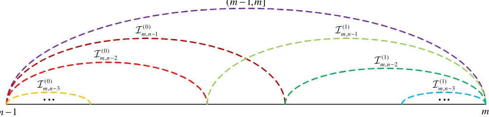
relationship ofIm,j(b) for differentj andb is illustrated by Fig. 3. It is easy to see that Im,j(b) ⊂ Im,j(b)0 for j < j0. It can be seen that because|τ0(b)|>1,Im,(b)0=∅for all m∈ {1,2,3}. In addition, we can find that |Im,j(b)| is indeed nondecreasing w.r.t. j.
C. Link between Atom and Risky Interval
According to the definitions of βj(b) and Im,j(b), we can easily link them as
βj(b) =
2nR−1
X
m=0
Pr{ds(Xn)e=m|Xj =b}p(Im,j(b)|m, b),
(25) where
p(Im,j(b)|m, b),Pr{s(Xn)∈ Im,j(b)|ds(Xn)e=m, Xj =b}. (26) It is easy to see that in the asymptotic sense,i.e., as n→ ∞,
p(Im,j(b)|m, b)→
R
{qnI(b) m,j}
f0,j(u|b)du
Rmqn
(m−1)qnf0,j(u|b)du
, (27)
where f0,j(u|b) is the conditional CCS given Xj = b (see Sect. III) and{qn
Im,j(b)}denotes a scaled version ofI
(b)
m,j (see theNotationpart of Sect. I for the definition ofinterval scaling
operation). Asnincreases,((m−1)qn, mqn]will converge to a real number. Hence, for nsufficiently large, f0,j(u|b)will be approximately uniform over ((m−1)qn, mqn] and
p(Im,j(b)|m, b) → |q
n
Im,j(b)|
|((m−1)qn, mqn]| =|I
(b)
m,j|
= (1−(1−q)qj−n)+, (28)
wherej∈[0 :n). Equivalently,
p(Im,n−j(b) |m, b)→(1−(1−q)q−j)+, (29)
...
...
(m−1,m]
(0)
, 3
m n−
I
(0)
, 1
m n−
I
(1)
, 2
m n−
I (1)
, 1
m n−
I
1 m
− m
(1)
, 3
m n−
I (0)
, 2
m n−
[image:7.612.57.559.60.180.2]I
Fig. 3. Illustration of risky intervalIm,j(b) forq= 1/√2. The horizontal axis iss(xn).
D. Calculation of Code HDS
After knowing atoms, we can obtain molecules ωn−j →
(1−(1−q)q−j)+, wherej∈[1 :n]. In turn, we can obtain
the code HDS as below
ψn,R(1)→ n
X
j=1
(1−(1−q)q−j)+. (30)
Finally, we can obtain the asymptotic code HDS as below
λR(1) = ∞
X
j=1
(1−(1−q)q−j)+. (31)
VI. MATHEMATICALCALCULATION OFψn,R(d)FORd≥2 One can easily extend the method developed in Sect. V to the general cased≥2. This section will first expandψn,R(d) as the sum ofatoms, then define therisky intervalto calculate atoms, and finally give the expression for ψn,R(d).
A. Expansion of ψn,R(d)as Sum-of-Atoms
Given dH(Xn,X˜n) = d, there are nd different XOR patterns between Xn and X˜n. Let j
, (j1,· · · , jd), where
0 ≤j1 <· · · < jd < n. The XOR pattern between Xn and
˜
Xn must take the form of
zn(j)
,(0j1,1,0j2−j1−1,· · ·,0jd−jd−1−1,1,0n−jd−1).
(32) In other words, zj1(j) =· · ·=zjd(j) = 1andzi(j) = 0for
other i /∈ j, where zi(j) denotes the i-th element of zn(j). Beginning withj1∈[0 : (n−d)], we can obtainjd0 ∈(jd0−1:
n−d+d0)ford0
∈[2 :d] by recursion. Let us define
k(dj)(Xn),
n
˜
Xn:ds( ˜Xn)e=ds(Xn)eand (Xn⊕X˜n) =zn(j)o
(33)
andωj ,E[k( j)
d (Xn)]. Then we can expand ψn,R(d)as
ψn,R(d) = n−d
X
j1=0
· · ·
n−1 X
jd=jd−1+1
ωj. (34)
Let Xj , (Xj1,· · · , Xjd) andb ,(b1,· · ·, bd) ∈ B
d, then we can further expand ωj as ωj = 2−dP
1d
b=0dβj(b), where βj(b),E[k
(j)
d (Xn)|Xj =b].
B. Length of Risky Interval
According to (3), given (Xn
⊕X˜n) = zn(j), we have
s( ˜Xn) = s(Xn) +τj(b), where b
∈Bd is the value of Xj
and
τj(b),(1−q)
d
X
d0=1
(−1)bd0qjd0−n. (35)
GivenXj =bandds(Xn)e=m∈[1 : 2nR), the necessary
and sufficient condition for the existence of a binary vector
˜
Xn in the m-th codebook satisfying ( ˜Xn
⊕Xn) =zn(j) is
s(Xn)
∈ Im,(b)j, where
Im,(b)j ,{((m−1), m]−τj(b)} ∩((m−1), m]. (36)
Let us define
(
δj−(b),min (1,(|τj(b)| −τj(b))/2)
δj+(b),min (1,(|τj(b)|+τj(b))/2)
. (37)
It is easy to obtain the risky interval
Im,(b)j =
(m−1) +δ−j(b), m−δ + j(b)
i
. (38)
Obviously, Im,(b)j = ∅ if |τj(b)| ≥ 1. The length of I (b)
m,j is |Im,(b)j|= (1− |τj(b)|)+.
C. Link between Atom and Risky Interval
According to the definitions of βj(b) andI (b)
m,j, we have
βj(b) = 2nR−1
X
m=0
Pr{ds(Xn)
e=m|Xj =b}p(I (b)
m,j|m,b),
(39) where
p(Im,(b)j|m,b),Pr{s(Xn)∈ Im,(b)j|ds(Xn)e=m, Xj =b}.
(40) In the asymptotic sense,
p(Im,(b)j|m,b)→ |I (b)
m,j|= (1− |τj(b)|)
+. (41)
Let(n−j),(n−j1,· · ·, n−jd)for1≤j1<· · ·< jd≤n, then (41) is equivalent to
where
ρj(b),
d
X
d0=1
(−1)bd0q−jd0. (43)
Therefore, for nsufficiently large,
βn−j(b)→(1−(1−q)|ρj(b)|)+. (44)
After a simple deduction, we obtain the tight ranges ofjd0 in (43) as follows: j1 ∈ [1 : (n−d+ 1)] and jd0 ∈ (jd0−1 : (n−d+d0)] ford0
∈[2 :d].
D. Calculation of Code HDS
After knowing atoms, we can obtain molecules as below
ωn−j →2−d 1d
X
b=0d
(1−(1−q)|ρj(b)|) +
, (45)
where1≤j1<· · ·< jd≤n. In turn, we can obtain the code HDS as below
ψn,R(d)→2−d n−d+1
X
j1=1
· · ·
n
X
jd=jd−1+1
1d
X
b=0d
(1−(1−q)|ρj(b)|)+.
(46) Finally, we can obtain the asymptotic code HDS as below
λR(d) = 2−d ∞
X
j1=1
· · ·
∞
X
jd=jd−1+1
1d
X
b=0d
(1−(1−q)|ρj(b)|)+.
(47)
VII. COMPLEXITY OFCALCULATINGDAC HDS
The complexity of (46) is O( nd
2d). To reduce the com-plexity, we exploit the fact ρj(b) =−ρj(1d⊕b)to obtain
ψn,R(d) = 21−d n−d+1
X
j1=1
· · ·
n
X
jd=jd−1+1
(0,1d−1)
X
b=0d
(1−(1−q)|ρj(b)|)+.
(48) Therefore, in the following, the leading bit of b will always be 0 without explicit declaration. Though the complexity of (46) is now reduced toO( nd
2d−1), it is still unacceptable for
largenandd. Thus the proposed method is feasible only for small nandd.
The complexity of (48) can further be reduced by swapping the order of summations
ψn,R(d) = 21−d
(0,1d−1)
X
b=0d
θ(b), (49)
whereθ(b),Pn
jd=dη(b, jd)and further
η(b, jd), jd−1
X
jd−1=d−1
· · ·
j2−1
X
j1=1
(1−(1−q)|ρj(b)|)+. (50)
The complexity of θ(b) isO( nd
), still high for large nand
d. However, we find that in some special cases,η(b, jd)≡0 for all jd > J(b), where J(b) is an integer totally de-pending on q while unrelated to n. Thus, we can obtain
θ(b) = PJ(b)
jd=dη(b, jd), whose complexity is O(
J(b)
d
). For
n J(b), the complexity of θ(b) will be significantly reduced.
The trick for findingJ(b)is to make|ρj(b)| ≥ (1−q)−1
for alljd> J(b). However, up to now, this problem is solved only for the special case that there is no more than one 1 in
b, while still remains open for the general case. To facilitate the description, we divide the case that there is no more than one1inbinto three subcases:
• bis an all-0 vector, i.e.,b= 0d;
• there is only one0before the1inb,i.e.,b= (0,1,0d−2); • there are two or more 0s before the 1 in b, i.e., b =
(0a,1,0d−a−1), where a ≥2.
We list the expressions of J(b) and θ(b) in the above three subcases in Tab. IV, while the detailed deductions are placed in the Appendix.
Below we will give some examples of J(b) and θ(b) in special cases by looking up Tab. IV and discuss the existence of J(b) in general cases. Afterwards, we will propose an approximation ofψn,R(d)for largenandd, and finally justify the practical values of (46).
A. Examples in Special Cases
1) Examples whenb= 0d: Ford= 1, by looking up Tab. IV, we can obtain
J(0) =blogq(1−q)c
θ(0) =
J(0) X
j=1
1−(1−q)q−j . (51)
Ford= 2, by looking up Tab. IV, we can obtain
J(02) =blogq(1−q)−logq(2−q−1)c
θ(02) =
J(02)
X
j2=2
j2−1
X
j1=1
1−(1−q)(q−j2+q−j1) . (52)
2) Examples whenb= (0,1,0d−2): Ford= 2, by looking
up Tab. IV, we can obtain
J(01) =b2 logq(1−q)c
θ(01) =
J(01) X
j2=2
j2−1
X
j1=1
1−(1−q)(q−j2−q−j1) . (53)
Ford= 3, by looking up Tab. IV, we can obtain
J(010) =b2 logq(1−q)−logq(2−q−1)c
θ(010) =
J(010) X
j3=3
j3−1
X
j2=2
j2−1
X
j1=1
1−(1−q)(q−j3−q−j2+q−j1) .
(54)
3) Examples when b = (0a,1,0d−a−1) and a ≥ 2: For d= 3anda= 2, by looking up Tab. IV, we can obtain
J(001) =blogq(1−q)−logq(2q−1−q−2)c
θ(001) =
J(001) X
j3=3
j3−1
X
j2=2
j2−1
X
j1=1
1−(1−q)(q−j3+q−j2−q−j1) .
TABLE IV EXAMPLE OFJ(b)ANDθ(b)
Term Expression
J(0d) jlog
q(1−q)−logq(2−q1−d) k
J(010d−2) j2 log
q(1−q)−logq(2−q2−d) k
J(0a10d−a−1) j−log q
(2−q1−d)(1−q)−1+ 2qa−dk
θ(0d)
J(0d)
X
jd=d jd−1
X
jd−1=d−1
· · · j2−1
X
j1=1
1−(1−q) d X
d0=1
q−jd0
!
θ(010d−2)
J(010d−2) X
jd=d
jd−1
X
jd−1=d−1
· · · j2−1
X
j1=1
1−(1−q) d X
d0=1
q−jd0−2q−jd−1
!!
θ(0a10d−a−1)
J(0a10d−a−1) X
jd=d
jd−1
X
jd−1=d−1
· · · j2−1
X
j1=1
1−(1−q) d X
d0=1
q−jd0−2q−ja+1
!!
B. Discussions in General Cases
As shown above, if the leading bit ofbis0andbcontains no more than one1, there will exist an integerJ(b)unrelated to
n such thatη(b, jd)≡0for alljd> J(b). The secret hidden behind it is that ρj(b) is always positive in this case. On the
contrary, if there are more than one1s inb, the positiveness of
ρj(b)cannot be guaranteed so that it is unknown whether there
still exists an integerJ(b)unrelated tonsuch thatη(b, jd)≡0 for all jd > J(b). Through many experiments, we find that
η(b, jd)usually tends to zero as jd increases. Thus, in most cases, there exists an integer J(b) unrelated to n such that
η(b, jd) ≡ 0 for all jd > J(b). However, we are not able to prove this conjecture. Note that, if J(b) exists, the two codewordsXnandX˜nbelonging to the same codebook differ from each other only in the lastJ(b)symbols.
C. Approximation of ψn,R(d)for largenandd
The complexity of calculatingψn,R(d)by (46) is unaccept-able for large n and d, so we give below a simple method to calculate the approximation of ψn,R(d)for largenand d. Let Xn and X˜n be two binary sequences belonging to the same codebook. As dH(Xn,X˜n) =dincreases,Xn andX˜n will become less correlated. Thus, for a large d,Xn andX˜n can be taken as two binary sequences that are independently drawn fromBn. This means: Fordsufficiently large,ψn,R(d) can be well approximated by the scaled combination formula
ψn,R(d)≈
n
d
Z 1
0
f02(u)du
2n(1−R), (56)
whereR01f2 0(u)du
2n(1−R)is in fact the average codebook
cardinality [24].
D. Practical Values of the Proposed Method
To obtain a complete HDS by (46), one must try all possible source sequences xn ∈
Bn and all possible XOR patterns zn ∈
Bn. Actually, by the Monte-Carlo method, one may
obtain an approximate HDS much faster. Naturally, one may ask: Does the proposed method make sense in practice? Our answer is YES. There are two reasons for this answer.
First, the decoding failures of DAC codes come mainly from closely-packed (in Hamming distance) codewords in each codebook (cf. Fig. 7(a) in Subsect. IX-D), so it is unnecessary to calculate the exact value of ψn,R(d) for large d by (46). Though the complexity of computingψn,R(d)by (46) is rather high for larged, it is very low for smalld(much faster than the Monte-Carlo method). Hence, the proposed method is useful in practice.
Second, the proposed method may be used to compute the FER of DAC codes. Let yn be the SI available only at the decoder and xˆn be the recovered version of xn. If we assume that xn−1 is known at the decoder, then ˆ
xn−1 = xn−1. Let Pr
{e} be the FER and Pr{e|xn−1 } be the conditional FER given xn−1 known at the decoder, then Pr{e|xn−1
}= Pr{xˆn−16=xn−1} andPr{e|xn−1}<Pr{e}.
Givenxn
∈ Cm,cn=xn⊕(0n−1,1)may or may not belong to Cm. If cn ∈ C/ m, the decoding will always be correct, regardless ofyn−1; otherwise,i.e., ifcn∈ Cm, the correctness of the decoding purely depends onyn−1. Therefore,
Pr{e|xn−1}= Pr{cn∈ Cm} ·Pr{yn−16=xn−1}. (57)
It is easy to obtain
Pr{cn∈ Cm}= Pr{s(xn)∈ Im,n−(b) 1}. (58)
LetPr{X 6=Y}=. By (29), we can obtainPr{e|xn−1 } → (2−2R) as n
→ ∞, which is just the lower bound given in [24]. The above method can be extended to more complex cases, i.e., all but the last n0 >1 symbols of each sequence are known at the decoder. When n0 = n, Pr{e|xn−n0} =
Pr{e}. Actually, the residual errors of DAC codes happen mainly at sequence tails (cf. Fig. 7(b) in Subsect. IX-D), so Pr{e|xn−n0} may be very close to Pr{e} for n0 n. Therefore,Pr{e|xn−n0
}, wheren0
n, may be taken as an approximation ofPr{e} and the complexity of computing the FER of DAC codes is significantly reduced.
VIII. CONVERGENCY OFDAC HDS
in general is NO. However, we will show below that ford= 1
and2, the answer is YES.
In the case of d= 1, according to the analysis in Subsect. VII-A, we can obtain
λR(1) = J(0) X
j=1
1−(1−q)q−j
, (59)
where J(0) is given by (51). Apparently, λR(1) < ∞, i.e.,
λR(d)converges ford= 1.
In the case of d= 2, according to the analysis in Subsect. VII-A, we can obtain
λR(2) = 1
2
J(00) X
j2=2
j2−1
X
j1=1
1−(1−q)(q−j2+q−j1)+
J(01) X
j2=2
j2−1
X
j1=1
1−(1−q)(q−j2
−q−j1)
, (60)
where J(00) andJ(01) are given by (52) and (53), respec-tively. Apparently, λR(2) < ∞, i.e., λR(d) converges for
d= 2.
The convergency of ψn,R(d) for d ≥ 3 is unknown. However, we have found that ψn,R(d) may not converge in some cases. For example, ifd= 3 andq= (√5−1)/2, it is easy to verify (q−j3−q−(j3−1)−q−(j3−2))≡0 and thus
(1−(1−q)|q−j3
−q−(j3−1)
−q−(j3−2)
|)+≡1. (61)
Therefore,
θ(011) =
n
X
j3=3
j3−1
X
j2=2
j2−1
X
j1=1
(1−(1−q)|q−j3−q−j2−q−j1|)+
>
n
X
j3=3
(1−(1−q)|q−j3−q−(j3−1)−q−(j3−2)|)+
= n−2. (62)
Asngoes to infinity,θ(011)will tend to infinity,i.e.,ψn,R(d) does not converge for d= 3if q= (√5−1)/2.
IX. EXPERIMENTALRESULTS
We implemented (46) in MATLAB to calculate the theo-retical values of ψn,R(d)and the DAC codec in C language to obtain the empirical values of ψn,R(d). Since DAC HDS does not depend on SI, we ignored SI in implementation for simplicity. We first generated a length-nequiprobable binary sequence as the source and compressed it by the DAC encoder. Then, the DAC decoder parsed the bitstream through a depth-first full search that was implemented by a recursive function. For eachd∈[0 :n], the decoder counted the number of paths that were d-away (in Hamming distance) from the source. For fairness, 103 trials were run and the average number of
paths that were d-away from the source was output as the empirical value of ψn,R(d). The precision of the used DAC codec was 32-bit. Four experiments were conducted to study the properties of DAC codes from different aspects.
TABLE V
COMPARISON OFTHEORETICAL ANDEMPIRICALVALUES OFΓn
R 2/6 3/6 4/6 5/6
TheoreticalΓn 1.6094 1.3046 1.1394 1.1677
EmpiricalΓn 1.6121 1.3071 1.1384 1.1675 R1
0 f2(u)du 1.6147 1.3047 1.1340 1.1541
A. Correctness Verification of (46)
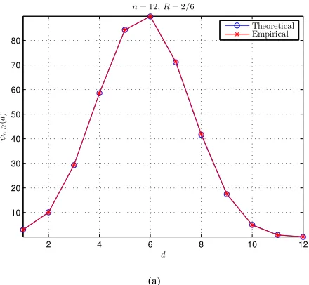
The aim of the first experiment is to verify the correctness of (46), which was achieved by comparing the theoretical values ofψn,R(d)with its empirical values. Some results for code lengthn= 12are presented in Fig. 4. Notice that since
ψn,R(0)≡1, it is not plotted in Fig. 4. We tested four different code rates:R= 2/6,3/6,4/6, and5/6, but only the results for
R= 2/6and5/6are included in Fig. 4 for conciseness. It can be seen that the theoretical values of ψn,R(d) coincide with its empirical values perfectly, which confirms the correctness of (46). Similar results are obtained for different values of n
andR.
In addition, we calculated the theoretical values ofΓnusing (15) and its empirical values by experiments. The results are listed in Tab. V, where the numerical values of R01f2(u)du,
which were obtained through the numerical algorithm in [23], are also included. It can be seen that the theoretical values of
Γn, the empirical values of Γn, and the numerical values of
R1 0 f
2(u)du are very close to each other. These findings also
confirm the correctness of (46).
B. Convergency of DAC HDS
The aim of the second experiment is to study the conver-gency of DAC HDS, which was achieved by trying different code lengths n ranged from 12 to 28. Both theoretical and empirical values ofψn,R(d)are plotted in Fig. 5. Considering the computational complexity, only the results of d = 1, 2, and 3 are included in Fig. 5. To show how code rate R
impacts the convergency of DAC HDS, two special code rates
R = 0.5 and log2[( √
5−1)/2] were tried. From Fig. 5, it can be seen that the theoretical values of ψn,R(d) coincide with its empirical values perfectly. Ford= 1and2,ψn,R(d) remains constant as code length n increases, i.e., ψn,R(d) converges asn goes to infinity. For d= 3, ψn,R(d)remains constant when code rate R = 0.5 while grows continuously when R = log2[(
√
5−1)/2] as n increases. Therefore, the convergency of ψn,R(d)for d≥3 depends on code rate: At some code rates,ψn,R(d)may tend to infinity as code length increases,i.e., does not converge. This property of DAC codes is very different from that of random codes because according to thelaw of large numbers (LLN), for any d <∞,ψn,R(d) of random codes will tend to0as code length goes to infinity.
C. Comparison of DAC Codes with Other Codes
2 4 6 8 10 12 10
20 30 40 50 60 70 80
d ψn
,R
(
d
)
n= 12,R= 2/6
Theoretical Empirical
(a)
2 4 6 8 10 12
0.1 0.2 0.3 0.4 0.5 0.6 0.7
d ψn
,R
(
d
)
n= 12,R= 5/6
Theoretical Empirical
[image:11.612.66.286.61.264.2](b)
Fig. 4. Correctness verification of (46) forn= 12. (a)R= 2/6. (b)R= 5/6.
12 14 16 18 20 22 24 26 28
1 1.5 2 2.5 3 3.5 4 4.5 5 5.5 6
n ψn
,R
(
d
)
R= 1/2
Theoretical,d= 1 Theoretical,d= 2 Theoretical,d= 3 Empirical,d= 1 Empirical,d= 2 Empirical,d= 3
(a)
12 14 16 18 20 22 24 26 28 0
1 2 3 4 5 6 7
n ψn
,R
(
d
)
R= log2[(
√5 −1)/2]
Theoretical,d= 1 Theoretical,d= 2 Theoretical,d= 3 Empirical,d= 1 Empirical,d= 2 Empirical,d= 3
[image:11.612.65.284.307.508.2](b)
Fig. 5. Convergency of DAC HDS. (a)R= 0.5. (b)R= log2[(√5−1)/2].
each codebook obey the binomial distribution, soψn,R(d)can be calculated by (56). It can be seen that at low rates, the HDS of DAC codes is similar to that of random codes, while at high rates, the HDS of DAC codes is different from that of random codes. Similar results are also obtained for different values of
n andR.
For turbo codes, the Fano algorithm was modified to com-pute the HDS in [28], where some examples of selected turbo codes with short interleaving were given. For a rate-0.5turbo code based on the (7,5) recursive systematic convolutional
(RSC) code with 8×8 nonuniform interleaving, the HDS is
w(8) = 0.34,w(9) = 1.5,w(10) = 0.63,w(11) = 0.12, and
w(12) = 1.71. Theminimum Hamming distance(MHD) is8.
For LDPC codes, the nearest nonzero codeword search
(NNCS) algorithm was proposed to find the MHD and multi-plicity in [29], where the results for some well-known LDPC
codes were reported. For the (3,6)-regular (504,252) and
(1008,504) MacKay codes [30], the MHDs are 20 and 34, and the multiplicities are2 and1, respectively. For thep-11
Margulis code [31], the MHD is40and the multiplicity is66. For the (13,5) and (17,5) Ramanujan-Margulis codes [32], the MHDs are14and24, and the multiplicities are2184and
204, respectively.
From the above results, we can find that compared to ran-dom codes, turbo codes, and LDPC codes, the main drawback of DAC codes is that the MHD is almost always1, regardless of code length n and rate R. This is because for d < ∞,
ψn,R(d)of DAC codes does not converge to0as code length
n goes to infinity (refer to Sect. VIII for the examples of
5 10 15 20 2000
4000 6000 8000 10000 12000 14000 16000
d ψn
,R
(
d
)
n= 24,R= 2/6
Random codes DAC codes
(a)
5 10 15 20
0 0.5 1 1.5 2 2.5
d ψn
,R
(
d
)
n= 24,R= 5/6
Random codes DAC codes
[image:12.612.61.542.61.266.2](b)
Fig. 6. Comparison of the HDS of DAC codes with that of random codes forn= 24. (a)R= 2/6. (b)R= 5/6.
to infinity because ψn,R(d) will tend to zero for anyd <∞ according to the LLN. In addition, it can be seen thatψn,R(d) of DAC codes is greater than that of random codes for smalld
while smaller than that of random codes for larged, implying that the HDS of DAC codes is inferior to that of random codes (especially at high rates). Based on these results, it can be concluded that the pureDAC codes (mapping all symbols of each sequence onto overlapped intervals) should be worse than random codes, turbo codes, and LDPC codes.
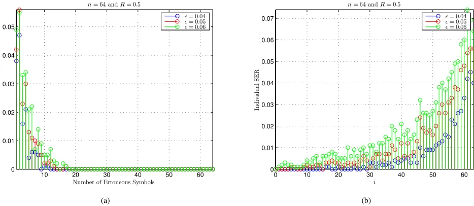
D. Properties of Decoding Errors
Let us first study the property of frame errors. In Fig. 7(a), we plot the occurrence rate of d-errors frames, wheren= 64
and R = 0.5. For clarity, the occurrence rate of error-free frames is not included in Fig. 7(a). It can be seen that most of erroneous frames include only very few erroneous symbols, implying that DAC decoding errors are caused mainly by closely-packed codewords within the same codebook.
Next we study the property of symbol errors. It is pointed out in Subsect. VII-B that the two codewords belonging to the same codebook differ mainly in the last few symbols, so symbol errors should happen mainly at the tail of each frame. To verify this point, we investigate how the error probability of each symbol is impacted by its position in a frame. For
n = 64 and R = 0.5, the individual SER of each symbol versus its index i is plotted in Fig. 7(b). It can be seen that symbol errors are not uniformly distributed over i∈ [0 : n)
and most of symbol errors do happen at the last few symbols of each frame, as reported in [15], [16].
The above phenomena inspire some improvements of DAC codes, e.g., permutating codewords in each codebook [24], mapping the last few symbols of each sequence onto non-overlapped intervals [15], [16], [27],etc.After these improve-ments, DAC codes may outperform LDPC codes and turbo codes, especially for short sequences [15], [16], [24], [27]. These improvements are all based on the principle of refining
the HDS of DAC codes by sparsifying the last few levels of DAC decoding trees. In such a way, closely-packed codewords in each codebook can be removed,i.e.,ψn,R(d)→0for small
d.
X. CONCLUSION
The analysis of DAC codes is an interesting and chal-lenging task. By extending our previous work, this paper makes another step forward. We define Hamming distance spectrumto describe how DAC codebooks are constructed and propose a method to calculate DAC HDS by the mathematical means. The correctness of the proposed method is verified by experiments. We also show how DAC codes can be improved from the viewpoint of HDS.
Despite the above advances, many important questions regarding DAC HDS,e.g., complexity, convergency,etc., still remain open. First, under which conditions will the HDS converge as code length increases? Second, if the HDS does converge as code length increases, can we find some way to calculate the HDS with linear or near-linear complexity? Third, if the HDS does not converge, how fast will it grow as code length increases? These difficult problems will be tackled in the future. Finally, another big challenge is the generalization of DAC HDS to nonuniform binary sources and even non-binary sources.
APPENDIX
A. Deduction of J(b)
1) Special Case ofb= 0d: In this case, sincej
d0 ≥d0 for alld0∈[1 :d], we have
ρj(b) =
d
X
d0=1
q−jd0 ≥q−jd+
d−1 X
d0=1
q−d0 !
10 20 30 40 50 60 0
0.01 0.02 0.03 0.04 0.05
Number of Erroneous Symbols
O
cc
u
rr
en
ce
R
a
te
n= 64 andR= 0.5
ǫ= 0.04 ǫ= 0.05 ǫ= 0.06
(a)
0 10 20 30 40 50 60 0
0.01 0.02 0.03 0.04 0.05 0.06 0.07
i
I
n
d
iv
id
u
a
l
S
E
R
n= 64 andR= 0.5
ǫ= 0.04
ǫ= 0.05
ǫ= 0.06
[image:13.612.72.539.63.266.2](b)
Fig. 7. Properties of DAC decoding errors, wheren= 64andR= 0.5. (a) Occurrence rate ofd-errors frames, wheredmeans the number of erroneous symbols in a recovered frame. (b) Individual SER versus symbol position.
A necessary condition for |ρj(b)|<(1−q)−1 is
q−jd < (1−q)−1−
d−1 X
d0=1
q−d0 !
= (2−q1−d)(1−q)−1, (64)
which is followed by jd<logq(1−q)−logq(2−q1−d).
2) Special Case of b = (0,1,0d−2): In this case, since jd0 ≥d0 for alld0 ∈[1 :d], we have
ρj(b) =
d
X
d0=1
q−jd0
!
−2q−jd−1
≥ q−jd−q−(jd−1)+
d−2 X
d0=1
q−d0
!
>0. (65)
A necessary condition for |ρj(b)|<(1−q)−1 is
q−jd(1−q) < (1−q)−1−
d−2 X
d0=1
q−d0 !
= (2−q2−d)(1−q)−1, (66)
which is followed by jd<2 logq(1−q)−logq(2−q2−d).
3) Special Case of b = (0a,1,0d−a−1) for a
≥ 2 and d ≥ 3: In this case, since jd0 ≥ d0 for all d0 ∈ [1 : d], we have
ρj(b) =
d
X
d0=1
q−jd0
!
−2q−jd−a
≥ q−jd+
d−1 X
d0=1
q−d0 !
−2qa−d>0. (67)
A necessary condition for |ρj(b)|<(1−q)−1 is
q−jd < (1−q)−1−
d−1 X
d0=1
q−d0 !
+ 2qa−d
= (2−q1−d)(1−q)−1+ 2qa−d, (68)
which is followed by jd <
−logq (2−q1−d)(1−q)−1+ 2qa−d
.
REFERENCES
[1] J. Rissanen, “Generalized Kraft inequality and arithmetic coding,”IBM J. Research & Development, vol. 20, no. 3, pp. 198–203, May 1976. [2] I. Witten, R. Neal, and J. Cleary, “Arithmetic coding for data
compres-sion,”Commun. of the ACM, vol. 30, no. 6, pp. 520–540, Jun. 1987. [3] P. Howard and J. Vitter, “Practical implementations of arithmetic
cod-ing,” in:Image and Text Compression, J. A. Storer, ed., pp. 85–112, Kluwer Academic Publishers, Boston, Mass, USA, 1992.
[4] C. Boyd, J. Cleary, S. Irvine, I. Rinsma-Melchert, and I. Witten, “Inte-grating error detection into arithmetic coding,”IEEE Trans. Commun., vol. 45, no. 1, pp. 1–3, Jan. 1997.
[5] B. Pettijohn, M. Hoffman, and K. Sayood, “Joint source/channel coding using arithmetic codes”,IEEE Trans. Commun., vol. 49, no. 5, pp. 826– 836, May 2001.
[6] T. Guionnet and C. Guillemot, “Soft and joint source-channel decoding of quasi-arithmetic codes,”EURASIP J. Applied Signal Process., no. 3, pp. 393–411, Mar. 2004.
[7] I. Sodagar, B. Chai, and J. Wus, “A new error resilience technique for image compression using arithmetic coding,” in:Proc. IEEE ICASSP, pp. 2127–2130, Istanbul, Turkey, Jun. 2000.
[8] T. Guionnet and C. Guillemot, “Soft decoding and synchronization of arithmetic codes: Application to image transmission over noisy channels,”IEEE Trans. Image Process., vol. 12, no. 12, pp. 1599–1609, Dec. 2003.
[9] S. Ben-Jamaa, C. Weidmann, and M. Kieffer, “Analytical tools for optimizing the error correction performance of arithmetic codes,”IEEE Trans. Commun., vol. 56, no. 9, pp. 1458–1468, Sep. 2008.
[10] D. Slepian and J. Wolf, “Noiseless coding of correlated information sources,” IEEE Trans. Inform. Theory, vol. 19, no. 4, pp. 471–480, Jul. 1973.
[11] J. Garcia-Frias and Y. Zhao, “Compression of correlated binary sources using turbo codes,” IEEE Commun. Lett., vol. 5, no. 10, pp. 417–419, Oct. 2001.
[12] A. Liveris, Z. Xiong, and C. Georghiades, “Compression of binary sources with side information at the decoder using LDPC codes,”IEEE Commun. Lett., vol. 6, no. 10, pp. 440–442, Oct. 2002.
[13] Y. Fang, “LDPC-based lossless compression of nonstationary binary sources using sliding-window belief propagation,” IEEE Trans. Com-mun., vol. 60, no. 11, pp. 3161–3166, Nov. 2012.
[14] Y. Fang, “Asymmetric Slepian-Wolf coding of nonstationarily-correlated
[15] M. Grangetto, E. Magli, and G. Olmo, “Distributed arithmetic coding,”
IEEE Commun. Lett., vol. 11, no. 11, pp. 883–885, Nov. 2007. [16] M. Grangetto, E. Magli, and G. Olmo, “Distributed arithmetic coding
for the Slepian-Wolf problem,” IEEE Trans. Signal Process., vol. 57, no. 6, pp. 2245–2257, Jun. 2009.
[17] X. Artigas, S. Malinowski, C. Guillemot, and L. Torres, “Overlapped quasi-arithmetic codes for distributed video coding,” in:Proc. IEEE ICIP, 2007, vol. II, pp. 9–12.
[18] S. Malinowski, X. Artigas, C. Guillemot, and L. Torres, “Distributed coding using punctured quasi-arithmetic codes for memory and mem-oryless sources,” IEEE Trans. Signal Process., vol. 57, no. 10, pp. 4154–4158, Oct. 2009.
[19] X. Chen and D. Taubman, “Distributed source coding based on punctured conditional arithmetic codes,” in:Proc. IEEE ICIP, pp. 3713– 3716, Sep. 2010.
[20] X. Chen and D. Taubman, “Coupled distributed arithmetic coding,” in:
Proc. IEEE ICIP, pp. 341–344, Sep. 2011.
[21] M. Grangetto, E. Magli, and G. Olmo, “Distributed joint source-channel arithmetic coding,” in:Proc. IEEE ICIP, 2010, pp. 3717–3720. [22] Y. Fang, “Distribution of distributed arithmetic codewords for
equiprob-able binary sources,” IEEE Signal Process. Lett., vol. 16, no. 12, pp. 1079–1082, Dec. 2009.
[23] Y. Fang, “DAC spectrum of binary sources with equally-likely symbols,”
IEEE Trans. Commun., vol. 61, no. 4, pp. 1584–1594, Apr. 2013. [24] Y. Fang and L. Chen, “Improved binary DAC codec with spectrum for
equiprobable sources,”IEEE Trans. Commun., vol. 62, no. 1, pp. 256– 268, Jan. 2014.
[25] J. Zhou, K. Wong, and J. Chen, “Distributed block arithmetic coding for equiprobable sources,” IEEE Sensors Journal, vol. 13, no. 7, pp. 2750–2756, Jul. 2013.
[26] A. Gamal and Y. Kim, “Network information theory,” Cambridge University Press, 2012.
[27] Y. Fang, V. Stankovic, S. Cheng, and E.-H. Yang, “Depth-first decoding of distributed arithmetic codes for uniform binary sources,” submitted toIEEE Trans. Commun.
[28] R. Podemski, W. Holubowicz, C. Berrou, and G Battail, “Hamming distance spectra of turbo-codes,” Annals of Telecommunications, vol. 50, no. 9–10, pp. 790–797, Sep.-Oct., 1995.
[29] X. Hu, M. Fossorier, and E. Eleftheriou, “On the computation of the minimum distance of low-density parity-check codes,” in:Proc. IEEE Int’l Conf. Commun., vol. 2, pp. 767–771, Jun. 2004.
[30] D. MacKay, “Good error-correcting codes based on very sparse matri-ces,”IEEE Trans. Inform. Theory, vol. 45, no. 3, pp. 399–431, Mar. 1999.
[31] G. Margulis, “Explicit constructions of graphs without short cycles and low density codes,”Combinatorica, vol. 2, no. 1, pp. 71–78, Jan. 1982. [32] J. Rosenthal and P. Vontobel, “Construction of LDPC codes based on Ramanujan graphs and ideas from Margulis,” in: Proc. 38th Annual Allerton Conf. Commun., Computing, and Control, Monticello, IL, Oct. 2000.
Yong Fangreceived his BEng, MEng, and PhD from Xidian University, Xi’an China, in 2000, 2003, and 2005, respectively, all in signal processing. Then, he was a post-doctoral fellow for one year with Northwestern Polytechnical University, Xi’an China. From 2007 to 2008, he joined Hanyang University, Seoul Korea, as a research professor. He is currently a full professor with Northwest A&F University, Shaanxi Yangling, China. He had long experiences in hardware system development,e.g., FPGA-based (Xilinx Vertex series) video codec design, DSP-based (TI C64 series) video surveilliance system, etc.. His research inter-ests include distributed source coding, joint source-channel coding, network information theory, and image/video coding, processing, and transmission.
Vladimir Stankovic(M03-SM10) received the Dr.-Ing. (Ph.D.) degree from the University of Leipzig, Leipzig, Germany in 2003. From 2003 to 2006, he was with Texas A&M University, College Station, first as Research Associate and then as a Research Assistant Professor. From 2006 to 2007 he was with Lancaster University. Since 2007, he has been with the Dept. Electronic and Electrical Engineering at University of Strathclyde, Glasgow, where he is cur-rently a Reader. He has co-authored 4 book chapters and over 160 peer-reviewed research papers. He was an IET TPN Vision and Imaging Executive Team member, Associate Editor of IEEE Communications Letters, member of IEEE Communications Review Board, and Technical Program Committee co-chair of Eusipco- 2012. Currently, he is Associate Editor of IEEE Transactions on Image Processing, IEEE Transactions on Communications, and Elsevier Signal Processing: Image Communication. His research interests include source/channel/network coding, user-experience driven image processing and communications and energy disaggregation.