An Examination of the Optimal Timing Strategy for a Slow Trader Investing in a High Frequency Trading Technology

An Examination of the Optimal Timing

Strategy for a Slow Trader Investing in a High

Frequency Trading Technology

Laura Delaney

July 6, 2015

Abstract

This paper examines, using a real options approach, the optimal time for

financial market investors to adopt a high frequency trading (HFT)

tech-nology. When the level of fast trading in the market is high, investors

should wait longer before adopting when the cost of the technology is

high, and vice versa. However, when the market is highly fragmented,

they should invest early (wait longer) when the cost of doing so is high

(low).

Furthermore, the equilibrium level of investment prescribed by the

model exceeds the socially optimal level, and investors should wait

longer (invest earlier) than the optimal time when the technology is

relatively cheap (expensive) in order to be more socially optimal.

∗_{Department of Economics, City University, Northampton Square, London, EC1V 0HB,}

Keywords: real options, high frequency trading, fragmented markets, welfare.

JEL Classification Numbers: C61, G1, G20, L1.

1

Introduction

This paper uses a real options approach to determine and analyse the

opti-mal time for financial market investors (referred to as “traders” hereafter) to

invest in a high frequency trading (HFT) technology. HFT is a type of

al-gorithmic trading that uses sophisticated computer algorithms to implement

vast amounts of trades in extremely small time intervals. The analysis is

mo-tivated by the fact that over the last decade, the state of financial markets

has changed considerably. In the first instance, markets have become highly

fragmented. There are now more than 50 trading venues for U.S. equities - 13

registered exchanges and 44 so called Alternative Trading Systems (see Biais

et al. [1] and O’Hara and Ye [14]). Hence, traders must search across many

markets for quotes and doing so can be costly as it may delay full execution

of their orders.

In response to the increase in market fragmentation, so called HFT

tech-nologies have been developed to reduce the associated costs borne by traders.

For example, traders can buy colocation rights (the placement of their

com-puters next to the exchange’s servers) which gives them fast access to the

ex-change’s data feed, they can invest in smart routers which can instantaneously

compare quotes across all trading venues and then allocate their orders

accord-ingly, or they can invest in high-speed connections to the exchanges via fiber

and so called pure-play HFT outlets are investing large sums of money into

such technologies in an effort to outpace the competition. Indeed, according

to Hoffmann [9], recent estimates suggest that HFTs are now responsible for

more than 50% of trading in U.S. equities.

In a recent paper, O’Hara [13] details the many ways in which market

mi-crostructure has changed over the past decade and calls for a new approach

to research in this area which “reflects the new realities of the high frequency

world”. Nevertheless, there has been a growth in the literature on HFT in

recent years, but much of this literature is empirical. On the whole, the

con-sensus has been that HFT improves liquidity (Hendershott et al. [8] and

Has-brouck and Saar [6]), is highly profitable (Menkveld [11]), and improves price

discovery (Hendershott and Riordan [7] and Brogaard et al. [2]).

The theoretical literature in this area is scant, but Biais et al. [1] develop a

model of HFT in a Glosten and Milgrom [4] type framework, which is the most

closely related model to the one in this paper. In particular, I incorporate the

HFT model of Biais et al. [1] into a real options framework such that the option

takes the shape of an exchange option where one payoff flow is exchanged for

another (see Smets [15] or Thijssen [16] for examples of “exchange-type” real

options models). This enables the optimal time for traders to invest in a HFT,

as a function of the level of HFT activity already accounted for in the market

as well as the degree of market fragmentation, to be determined analytically.

The analytical solution takes the form of a threshold policy: invest if the payoff

flow from adopting exceeds the threshold level, otherwise refrain from doing

so.

Since the seminal contribution by Myers [12], it has become quite standard

partially so) investment projects as real options. The main feature of real

options analysis is the recognition that the investor has the option to postpone

investing until some future date. Hence, the investor has some flexibility over

his investment decision which is not accounted for in classical Marshallian

investment evaluation. This flexibility has economic value (typically referred

to as the option value of waiting) owing to the irreversibility, and because the

payoff from investing is uncertain. Investing in the HFT technology is both an

irreversible and an uncertain investment, and can be entered into at any time.

Therefore, a real options approach is appropriate for evaluating this particular

investment decision. To the best of my knowledge, the approach has not been

previously applied in a HFT context, nor has the HFT issue been considered

from a timing perspective.

The novel contribution of the paper, from the real options perspective, is

the application of the methodology to the “new” market microstructure

envi-ronment of fragmented markets and HFTs. Hence, I restrict the examination

of the optimal policy to these two characteristics: When the cost of investing is

low, the threshold decreases in the level of HFT in the market and increases in

the level of market fragmentation. This is driven by the option value of waiting

which dominates the present value effect. However, when the cost of investing

is high, the present value effect dominates and the threshold increases in the

level of HFT and decreases in the degree of market fragmentation.

Finally, from a welfare perspective, adhering to the optimal policy

pre-scribed by the model yields an equilibrium level of HFT which always exceeds

that level which is socially optimal. Biais et al. [1] obtain a similar result in

their paper and analyse possible policy responses to this problem. For example,

on HFTs. The socially optimal level of HFT would be reached if the tax

im-posed is equal to the externalities generated by HFTs. Their analysis can be

implemented in the same way to this model by simply raising the total cost of

investing and the result would be the same. However, the model is solved from

an optimal timing perspective and this generates another response: in order

to be socially optimal, traders should wait longer before investing in the HFT

technology than the real options approach suggests when the cost of investing

is relatively low, and vice versa when this cost is high.

The remainder of this paper is organised as follows. The model is set up

and solved in the next section. Section 3 analyses the implications of the

model for investment timing and welfare, and Section 4 concludes. All figures

are placed in the appendix.

2

The Model

2.1

The Trading Environment

Consider a risk-neutral market trader contemplating investment in a HFT

tech-nology. Investing in the technology incurs a sunk costI >0. Before investing, the trader is a regular (slow) trader who trades in fragmented markets where

fast high frequency traders (HFTs) also trade. Hence, he is exposed to the

impact such traders have on the likelihood of his orders getting executed at

favourable prices. Once he invests, however, he becomes one of the HFTs.

I assume a similar market and trading environment to that of Biais et al. [1].

In particular, I capture a fragmented market where slow traders compete with

HFTs by assuming there is a size-one continuum of trading venues distributed

fractionλ <1 of the trading venues are “liquid”. In the context of this model, a trading venue is liquid if it allows the trader to fully execute his order at his

specified order price. At time t, the liquid venues are located on the circle in an interval of sizeλ, starting at a venuevtsuch thatvtis uniformly distributed

on the circle and i.i.d. across periods. Moreover, at any point in time there

are a continuum of traders in the market, some of which are HFTs and some

of which are slow. In order to execute his desired trade, a trader must find a

trading venue that is liquid. When a trader enters the market, he is uncertain

about which venues are liquid since he does not know vt.

HFTs have extremely fast connection speeds to the market and can observe

all venues instantaneously (Biais et al. [1]). Thus, they find a liquid one with

certainty upon arrival to the market. However, a slow trader must search for

liquid trading venues and finding one can take time. I assume that at each

point in time, a slow trader can only send orders to one trading venue on

the circle. His choice of venue is random and uniformly drawn from the unit

circle. Therefore, with probability λ the venue is liquid and the slow trader can execute his order. If it is not liquid, the trader cannot trade at t and with probability (1−ϕ) he will exit the market and not trade again. However, with probability ϕ, he waits and tries to trade again at the next time point t+dt. I denote byα (respectively 1−α) the mass of fast (resp. slow) institutions in the market at time t. Intuitively, and indeed is the case in the model of Biais et al. [1], an increase in the level of fast trading α reduces the expected gains of both fast and slow institutions. To capture this, I let the profit flow

dynamics from trading, (Xt)t≥0, for both a fast and a slow trader follow an arithmetic Brownian motion of the form

such that (Wt)_t≥0 is a standard Weiner process, and κ(α) ∈ (0,1) (for α ∈

(0,1)), κ′(α)<0 for all Xt≥0 and κ′(α)>0 for all Xt <0.

A fast trader is one who has already invested in the HFT technology and,

thus, all his orders are filled with certainty at the time of submission. Hence,

I assume that he earns a profit stream of (Xt)t≥0 with certainty.

A slow trader, however, must search for quotes and finding a liquid venue

can take time. For some arbitrary time t ≥ 0, he finds a liquid venue with probability λ((1−λ)ϕ)t. Thus, he obtains a profit of λ((1−λ)ϕ)tXt in each

period t.

If the current state of the profit flow process isx and the slow trader, who discounts profits at the rate r > 0, decides to adopt the HFT at the stopping time τ, then via the strong Markov property of diffusions, the value of this policy to the trader, denoted by V(x), is given by

V(x) =Ex

[∫ τ

0

λ((1−λ)ϕ)te−rtXtdt+

∫ _∞

τ

e−rtXtdt−e−rτI

]

=Ex

[∫ _∞

0

λ((1−λ)ϕ)te−rtXtdt

]

+Ex

[

e−rτF(Xτ)

]

,

= λκ(α)

r−ln((1−λ)ϕ)

(

x+ µ

r−ln((1−λ)ϕ)

)

+Ex

[

e−rτF(Xτ)

]

(2)

where

F(Xτ) =EXτ

[∫ _∞

0

(

1−λ((1−λ)ϕ)t)e−rtXtdt

]

−I

=κ(α)

r

(

Xτ +

µ r

)

− λκ(α)

r−ln((1−λ)ϕ)

(

Xτ +

µ

r−ln((1−λ)ϕ)

)

−I

(3)

is the trader’s payoff function from adoption, Ey denotes the expectation

that F(Xτ)>0.

The problem for the trader is to find a value functionV∗(x) and a stopping time τ∗ such that the following optimal stopping problem is solved:

V∗(x) :=Ex

[

e−rτ∗F(Xτ∗)

]

= sup

τ∈T

Ex

[

e−rτF(Xτ)

]

, (4)

for T the set of stopping times.

I show in the next subsection that there is a unique trigger X∗ such that adoption of the HFT is optimal as soon as X∗ is hit from below.

2.2

The Model Solution

Theorem 1. Let f :R→R be defined by

f(x) =e−β1x_F(x)

where β1 is the positive (real) root of the quadratic equation

Q(β)≡ 1

2(κ(α)) 2

σ2β2 +κ(α)µβ −r= 0. (5)

If f attains a unique maximum at X∗, then the optimal stopping problem (4)

is solved by

V∗(x) =

    

e−β1(X∗−x)_F(X∗_{) if x < X}∗

F(x) if x≥X∗.

(6)

Furthermore, the optimal stopping time is given by

Proof. Before I prove the theorem, I show that the function f :R → R has a maximiser which is unique.

f′(x) = 0⇐⇒F′(x) =β1F(x)

and x is a maximiser iff F′′(x) < β1F′(x). But, from (3), F′′(x) = 0 and

F′(x) > 0. Therefore, any solution to f′(x) = 0 is a maximiser since β1 > 0 also. Furthermore, since F(x) is linear in x, the solution to f′(x) = 0 has to be unique.

I next prove the result of the theorem using the conditions outlined in

Thijssen [17]. According to that paper, the conditions to be checked are as

follows:

1. The value function must dominate the payoff function; i.e., V∗ > F, 2. The value function is a smooth function; i.e., V∗ ∈C1_,

3.

LXV∗−rV∗ = 0

for all x < X∗. LX ∈C2 is the partial differential operator defined by

LXg(x) = lim t↓0

E[e−rt_g(X

t)]−g(x)

t

where g ∈C2_.

4. V∗ is superharmonic; i.e.,

LXV∗ −rV∗ ≤0

5. the family {V∗(Xτ)|τ ≤ τC} is uniformly integrable with respect to

(Px)x∈(−∞,∞), where τC = inf{t≥0|Xt ̸∈(−∞, X∗)}.

The conditions are verified as follows:

1. Let XN P V be such that F(XN P V) = 0. Since F′(x)>0 and F(X∗)>0

by assumption, it must be the case that X∗ > XN P V. For all x ∈

(−∞, XN P V], F(x)<0 and, thus, V∗(x)> F(x).

For all x∈[X∗,∞),V∗(x) = F(x).

Finally, for all x ∈ (XN P V, X∗), suppose V∗ < F. Then it must be the

case that

e−β1(X∗−x)_F(X∗_{)< F(x)}⇐⇒_e−β1X∗_F(X∗_{)< e}−β1x_F(x).

However, this condition cannot hold if X∗ is the unique maximiser of

f(x). Therefore, it must be the case that V∗ > F on (XN P V, X∗) also.

This proves that the value function dominates the payoff function.

2. It is clear that V∗ is continuous. Moreover, V∗ is differentiable at X∗

since

lim

x↑X∗V

∗_{(x) = lim}

x↑X∗β1e

−β1(X∗−x)_F(X∗₎

= lim

x↑X∗β1e

−β1(X∗−x)F

′_(X∗₎

β1

[from f′(X∗) = 0] =F′(X∗).

(8)

is equal to the partial differential operator

LXeg(x) = lim_t↓0

E[e−rt_g(X

t)]−g(x)

t =LXg(x)−rg(x)

=1

2(κ(α)) 2_σ2∂

2_g(x)

∂x2 +κ(α)µ

∂g(x)

∂x −rg(x).

For all x≤X∗,

∂V∗(x)

∂x =β1e

−β1(X∗−x)_F(X∗_{) and} ∂

2_V∗_(x)

∂x2 =β 2 1e−

β1(X∗−x)_F(X∗_),

then it follows from (5) that

LXeV∗(x) =

1

2(κ(α)) 2_σ2∂

2_V∗_(x)

∂x2 +κ(α)µ

∂V∗(x)

∂x −rV

∗_(x) =

(

1

2(κ(α)) 2_σ2_β2

1 +κ(α)µβ1−r

)

e−β1(X∗−x)_F(X∗₎

=0

(9)

as required.

4. For all x≥X∗

LXV∗−rV∗ =LXF −rF

=1 2(κ(α))

2

σ2F′′(x) +κ(α)µF′(x)−rF(x)

<

(

κ(α)µ− r β1

)

F′(x)

(10)

since F′′(x) = 0, and f′(x) < 0 and F(x) > 0 for x ≥ X∗. However, it is easy to check that (κ(α)µ−r/β1) < 0 and, since F′(x) >0, it must therefore be the case that LXV∗ −rV∗ < 0 for x ≥ X∗. Hence, V∗ is

superharmonic.

uniform integrability test function since g is increasing and con-vex in y and limy→∞g(y)/y = ∞ (see Thijssen [17]). Then the family

Y := {Yt ≤ YτC} is uniformly integrable with respect to (Py)y∈(−∞,∞) if sup_Yt∈YE[g(|Yt|)]<∞. Applying this to our function gives,

sup

t≤τC{

∫

g(|V∗(x)|)dPx}= sup x≤X(τC)

E[(V∗(x))2] = sup

x≤X(τC)

E[e−2β1(X∗−x)_](F(X∗₎₎2_]

≤(F(X∗))2 <∞

(11)

since X∗ > x for all t≤τC.

From the theorem, we get thatX∗ is given by

X∗ = 1

β1 −

Ψ(r, µ, λ, ϕ) + Φ(r, λ, ϕ, α)I, (12)

where

Ψ(r, µ, λ, ϕ) = µ

((1−λ)r−ln((1−λ)ϕ))

(

(r−ln((1−λ)ϕ))2_−λr2

r(r−ln((1−λ)ϕ))

)

and

Φ(r, λ, ϕ, α) = r(r−ln((1−λ)ϕ))

3

Model Implications

3.1

Investment Timing

Proposition 1. The more high frequency traders there are in the market,

the sooner a slow trader will invest in the HFT technology when the cost of

investing is low, but the longer he will wait when this cost is high.

To see this, consider the following equation:

∂X∗

∂α <0⇐⇒Φ(r, λ, ϕ, α)I <

1

β1

(13)

since X∗ >0 =⇒κ′(α)<0.

Proposition 1 says that an increase in the level of fast trading will lead

other slow traders to be more forthcoming with adopting the HFT technology

when the cost of doing so is relatively low. This result arises from the option

effect of waiting. When the cost of investing in the technology is relatively

low, the option effect dominates the present value effect (cf. equation (13)).

When α rises, the value of waiting decreases since a relatively low investment cost implies a high opportunity cost to waiting. Therefore, the slow traders

will be more forthcoming with investing. This result is depicted in Figure 1.

However, when the cost of investing is high, the present value effect

domi-nates the option effect and the condition given by (13) does not hold. A high

α reduces the present value from investing (arising from the assumption that high frequency traders reduce gains from trade) implying that the opportunity

cost of waiting is low and, hence, traders will be more reluctant to invest (see

To obtain an explanation for the observed results, I examine the relative

value of being fast. The relative value of being fast, denoted by ∆(α), is the amount by which the expected trading profits for high frequency traders,

denoted byVf_{(α), exceeds the expected trading profits for slow traders,V}s_(α):

∆(α) =Vf(α)−Vs(α) =Ex

[∫ _∞

0

(

1−λ((1−λ)ϕ)t)e−rtXtdt

]

−Ex

[∫ _∞

0

λ((1−λ)ϕ)te−rtXtdt

]

=κ(α)

r

(

x+µ

r

)

− 2λκ(α)

r−ln((1−λ)ϕ)

(

x+ µ

r−ln((1−λ)ϕ)

)

.

(14)

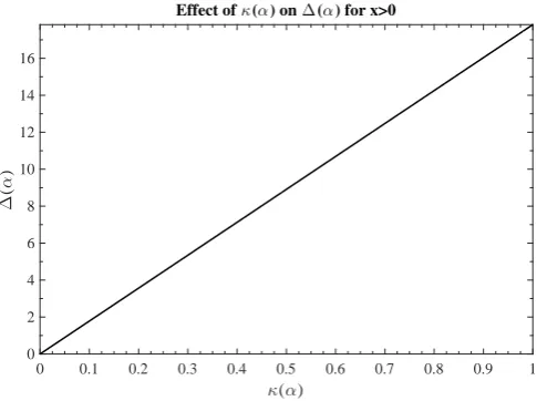
Since κ′(α) > 0 for all x < 0 and κ′(α) < 0 otherwise, the relative value of being fast decreases in α if and only if

∂∆(α)

∂κ(α) =

    

Positive if x≥0 Negative if x <0.

(15)

Indeed, from Figures 3 and 4, we see this is the case.

Therefore, an increase in the level of high frequency trading reduces the

relative value of being fast. When the cost of investing is low, the fall in the

value of waiting overshadows the effect of the fall in relative value of being

fast and traders are eager to avail of the low cost by adopting the technology

early. On the other hand, when this cost is high, the relative value of being

fast provides less compensation to the trader for incurring the high cost and,

moreover, this dominates the effect of a fall in the value of waiting. Therefore,

as we observe in Figure 2, the higher the level of fast trading, the more reluctant

is the trader to adopt the technology when the cost of doing so is high.

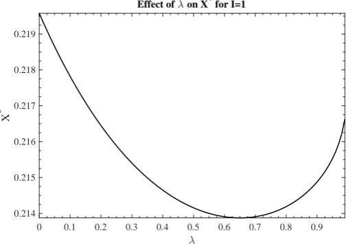
to the market fragmentation parameter λ. However, Figures 5 and 6 imply that X∗ is convex in λ when the cost of investment is low, and concave in λ

when the cost is high.

A high value of λ implies a low degree of market fragmentation and a relatively easier trading environment for a slow trader to find liquid venues.

Furthermore, the expected profitability of fast institutions increases in the

degree of market fragmentation,1 _{and so too does the relative value of being}

fast (this follows from equation (14)).

Accordingly, when the cost of investing in the technology is low, the option

effect on the optimal time to invest dominates the present value effect and an

increase in the level of market fragmentation will make the trader wait longer

before investing (see Figure 5) even though his expected profit from doing so

is higher. On the other hand, when the cost of investing is high, a higher level

of fragmentation actually speeds up investment. In this instance, the present

value effect dominates and, since the relative value of being fast is higher owing

to the more fragmented environment, this effect more than compensates the

trader for the high cost of investing implying he is willing to invest sooner and

incur the high cost. A possible explanation for this, as suggested by Biais et al.

[1] for a different but related effect in their model, is that the trader anticipates

that if it remains slow while others are fast, he will obtain very low profits as

the market gets more and more fragmented. Hence, the relative value of being

fast becomes more valuable and the sooner he will invest.

Furthermore, the convexity of the low cost effect implies that the more

fragmented the market becomes, the lesser is the positive impact on the value

of waiting since the marginal effect ofλon the optimal time to invest is positive.

The concavity of the high cost case, however, implies that the present value

effect is strengthened as the market becomes increasingly fragmented.

While I depict the impact ofαand λfor both high and low costs of invest-ment, the relatively high cost results are more pertinent because in practice,

trading firms invest massive amounts of money in high frequency technology.

For example, Laughlin et al. [10] estimate that achieving a 3-millisecond

de-crease in communication time between Chicago and New York markets costs

in the range of $500 million.

Finally, as shown in Theorem 1, the net present value threshold XN P V

asserts that investment in the high frequency technology should take place

earlier than the real options threshold suggests. This is one of the most widely

known and cited results in real options analysis and is typically driven by the

fact that the standard net present value theory of investment does not account

for uncertainty over future payoffs nor the fact that the investments are, at

least partially, irreversible (see, for example Dixit and Pindyck [3]). It also

assumes that investing is a now-or-never decision with no value of waiting.

The driving force in this model is the same as in standard models because,

since F(XN P V) = 0, whereF(x) is given by (3), it is easily verified that

X∗ −XN P V =

1

β1

,

and any term involvingβ1 pertains to the option effect, or the value of waiting. In the next subsection, I examine the welfare implications of adhering to

3.2

Welfare Implications of the Optimal Investment Time

So far, the level of fast trading in the marketαhas been exogeneous. However, in order to analyse the implications arising from the model for social welfare,

it is necessary to endogenise α. In order to do so, I assume in the customary way (see, for example, Grossman and Stiglitz [5], Hoffmann [9] and Biais et al.

[1]) that all traders are born slow but have the opportunity to become fast

at an exogeneously determined cost I > 0. Then, an interior equilibrium requires that traders are indifferent about being fast or slow; in other words,

that the relative value of being fast equals the cost of investing. Therefore, the

equilibrium level of fast trading α∗ is the value of α that solves

∆(α∗) =I.

Utilitarian welfare is equal to

W(α) = α(Vf(α)−I)+ (1−α)Vs(α)

and the socially optimal level of fast trading, denoted by α∗_SO, is the value of

α that maximises W(α). Thus α∗_SO solves

∆(α∗_SO)−I+α∗_SO∂V

f_(α)

∂α |α=α∗SO + (1−α

∗

S0)

∂Vs_(α)

∂α |α=α∗SO = 0. (16)

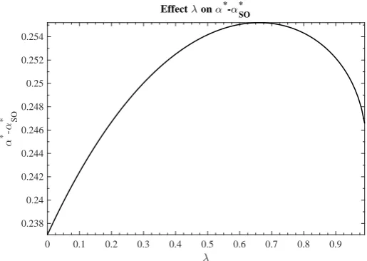
From Figure 7, it is clear that the equilibrium level of fast trading α∗, always exceeds the socially optimal level no matter how fragmented the market. This

is because the greater the level of high frequency trading in the market, the

lower the expected trading profit for slow traders and therefore, high frequency

internalise when making their investment decisions.

A similar result emerges from the models of Biais et al. [1] and Hoffmann

[9]. Since high frequency traders are a source of the negative externality,

both papers analyse possible policy responses to this problem. Hoffmann [9]

discusses the implications of imposing restrictions such as minimum resting

times for limit orders and undifferentiated limits to message traffic, while Biais

et al. [1] discuss the implications of imposing a ban on high frequency traders,

as well as providing an analysis of the effects a pigovian tax would have if

imposed on high frequency traders.

However, the optimal timing model in this paper provides a relatively more

straightforward response: in order to be socially optimal, traders should wait

longer before investing in the HFT technology than the real options approach

suggests when the cost of investing is relatively low, and vice versa when

this cost is high. This is because X∗ decreases (increases) in α when the cost of investing is low (high) owing to the option (present value) effect (cf.

Proposition 1).

4

Conclusion

In recent years, the state of market microstructure has changed considerably.

There are many ways in which these changes have come about (see O’Hara

[13] for a detailed description), but one of the biggest changes is that markets

have become highly fragmented. When markets are fragmented, traders must

search across many markets for venues which will execute their orders at their

specified prices. This can result in delayed or partial execution which is costly.

for speed by traders, and various types of expensive technologies have been

developed. Such technologies enable traders to compare all trading venue

instantaneously or obtain a glimpse of the true state of the market before

everyone else.

In this paper I derive a model, using techniques from real options analysis,

which provides insights into the optimal time traders should invest in high

frequency trading technologies. The model prescribes waiting longer when the

cost of the technology is very high and the level of high frequency trading

activity in the market is also high. On the other hand, when the cost is

relatively low, traders should adopt quickly when the level of fast trading is

high. Moreover, in a highly fragmented market environment, traders should

invest in the technology early when the cost of doing so is high, and vice versa

when this cost is low.

Finally, I show that the equilibrium level of investment prescribed by the

model is excessive from a social welfare perspective, and that in order to be

more socially optimal, traders should wait longer before investing in the HFT

technology than the model suggests when the cost of investing is relatively

low, and vice versa when this cost is high.

References

[1] B. Biais, T. Foucault, and S. Moinas. Equilibrium fast trading. Journal

of Financial Economics, forthcoming, 2015.

[2] J. Brogaard, T. Hendershott, and R. Riordan. High frequency trading

[3] A.K. Dixit and R.S. Pindyck. Investment under uncertainty. Princeton

University Press, Princeton, NJ, 1994.

[4] L. Glosten and P. Milgrom. Bid, ask, and transaction prices in a

special-ist market with heterogeneously informed traders. Journal of Financial

Economics, 14(1):71–100, 1985.

[5] S. Grossman and J. Stiglitz. On the impossibility of informationally

effi-cient markets. The American Economic Review, June:393–408, 1980.

[6] J. Hasbrouck and G. Saar. Low latency trading. available

at http://papers.ssrn.com/sol3/papers.cfm?abstract id=1695460,

2013.

[7] T. Hendershott and R. Riordan. Algorithmic trading and the market for

liquidity. Journal of Financial and Quantitative Analysis, 48(4):1001–

1024, 2013.

[8] T. Hendershott, C. Jones, and A. Menkveld. Does algorithmic trading

improve liquidity? Journal of Finance, 66(1):1–33, 2011.

[9] P. Hoffmann. A dynamic limit order market with fast and slow traders.

Unpublished working paper, European Central Bank, 2013.

[10] G. Laughlin, A. Aquirre, and J. Grundfest. Information

transmis-sion between financial markets in Chicago and New York. available at

https://economics.sas.upenn.edu/system/files/event papers/LAG final.pdf,

2014.

[11] A. Menkveld. High frequency trading and

http://papers.ssrn.com/sol3/papers.cfm?abstract id=1722924,

2013.

[12] S.C. Myers. Determinants of corporate borrowing. Journal of Financial

Economics, 5:147–176, 1977.

[13] M. O’Hara. High frequency market microstructure. Journal of Financial

Economics, In press, 2015.

[14] M. O’Hara and M. Ye. Is market fragmentation harming market quality?

Journal of Financial Economics, 100:459–474, 2011.

[15] F. Smets. Exporting versus FDI: The effect of uncertainty, irreversibilities

and stategic interactions. Unpublished working paper, Yale University,

1991.

[16] J.J.J. Thijssen. Premeption in a real option game with first mover

advan-tage and player-specific uncertainty. Journal of Economic Theory, 145:

2448–2462, 2010.

[17] J.J.J. Thijssen. An easy-to-use toolkit for solving optimal stopping

Appendix

A

Figures

α

0 0.1 0.2 0.3 0.4 0.5 0.6 0.7 0.8 0.9 1

X

*

0.05 0.1 0.15 0.2 0.25 0.3 0.35 0.4 0.45 0.5

Effect of α on X

*

for I=1

Figure 1: Parameter values: I = 1, ϕ = 0.5, λ = 0.5, κ(α) := 1 −0.75α,

α

0 0.1 0.2 0.3 0.4 0.5 0.6 0.7 0.8 0.9 1

X

*

1 1.1 1.2 1.3 1.4 1.5 1.6 1.7 1.8

Effect of α on X *

for I=10

Figure 2: Parameter values: I = 10, ϕ = 0.5, λ = 0.5, κ(α) := 1−0.75α,

σ = 0.2, r= 0.05, µ= 0.02.

κ(α)

0 0.1 0.2 0.3 0.4 0.5 0.6 0.7 0.8 0.9 1

∆

(

α

)

0 2 4 6 8 10 12 14 16

Effect of κ₍α_{) on} ∆₍α_{) for x>0}

Figure 3: Parameter values: x = 0.5, ϕ = 0.5, λ = 0.5, σ = 0.2, r = 0.05,

κ(α)

0 0.1 0.2 0.3 0.4 0.5 0.6 0.7 0.8 0.9 1

∆

(

α

)

-1.8 -1.6 -1.4 -1.2 -1 -0.8 -0.6 -0.4 -0.2 0

Effect of κ(α) on ∆(α) for x<0

Figure 4: Parameter values: x = −0.5, ϕ = 0.5, λ = 0.5, σ = 0.2, r = 0.05,

µ= 0.02.

λ

0 0.1 0.2 0.3 0.4 0.5 0.6 0.7 0.8 0.9

X

*

0.214 0.215 0.216 0.217 0.218 0.219

Effect of λ on X* for I=1

Figure 5: Parameter values: I = 1, ϕ = 0.5, α = 0.5, κ(α) := 1−0.75α,

λ

0 0.1 0.2 0.3 0.4 0.5 0.6 0.7 0.8 0.9

X

*

0.94 0.941 0.942 0.943 0.944 0.945 0.946 0.947

Effect of λ on X* for I=10

Figure 6: Parameter values: I = 10, ϕ = 0.5, α = 0.5, κ(α) := 1−0.75α,

σ = 0.2, r= 0.05, µ= 0.02.

λ

0 0.1 0.2 0.3 0.4 0.5 0.6 0.7 0.8 0.9

α

*

-α

* SO

0.238 0.24 0.242 0.244 0.246 0.248 0.25 0.252 0.254

Effect λ on α*-α* SO

Figure 7: The parameter values areI = 10,x= 0.5ϕ= 0.5,κ(α) := 1−0.75α,