Risk analysis of supply : comparative performance and short-term prediction

1 INTRODUCTION

1.1 Motivating industry problem

Our study has been driven by challenges facing sup-ply managers in several, similar manufacturing com-panies. The managers have responsibilities that span the life of a supplier, from procuring, developing, maintaining and/or exiting the relationship. The manufacturing companies are all responsible for the assembly of engineering systems for which the sub-assemblies and component parts are sourced from suppliers globally. The design authority for parts can reside with the manufacturer, the supplier or both.

The set of suppliers for the manufacturing compa-nies are continually in a state of change, with suppli-ers being exited and new ones being added. In addi-tion, the volume of work apportioned to each supplier changes over time depending on projects commissioned by end customers for bespoke engi-neering systems. The manufacturers produce highly complex products which are customised to varying degrees. The customisation together with limited holding space and resource implications means it is not possible to stock a spare of every type of part. Therefore, parts are ordered as needed.

On-time delivery of parts from suppliers to the re-quired functional and quality standard is necessary for the production of the final assembly so that the manufacturer meets end customer deadlines. How-ever problems such as production delays and disrup-tion arise when parts are delivered late or do not conform to requirement.

Heuristically the supply managers have an under-standing of the causes and modes of supplier failure to deliver parts to the correct specification at the right time. However, the managers do not have mod-els to support analysis that allows them to articulate and evidence the relationship between factors that drive supply risk and hence no reliable means of making prediction, even for relatively short-term planning horizons. The consequence is that there tends to be a reactive response to events that delay or disrupt supply. Our managers would like analytical models to provide them with predictions that would aid better risk management and provide evidence to inform their decisions.

1.2 Purpose of risk analysis

Our paper describes how we can use the empirical data about supplier characteristics and performance records typically held in enterprise resource systems to better understand and predict aspects of supplier risk. These data have been primarily recorded by the manufacturing companies to schedule production and manage operations. We show how such data might also be exploited to provide information to better manage risk in the supply process.

Our goal is to develop a modelling suite that sup-ports analysis of risk in different stages of supplier life so that managers with different levels of respon-sibilities can use the information appropriately. For example, the information gained from analysis could be used by supply managers: to predict late

deliver-Risk analysis of supply: comparative performance and short-term

prediction

L. Walls, J. Quigley, M. Parsa & E. Comrie

Department of Management Science, University of Strathclyde, Glasgow, Scotland

ies given loading and other factors affecting the sup-plier ability to deliver on time; to provide a robust comparative assessment of supplier performance for variables of interest, such as late delivery rates or non-conformance rates on past and ongoing projects; and to estimate how much it is worth investing in suppliers, new or established, through auditing and other activities to learn more about their capabilities to improve; predictions of the chance of being better off exiting a supplier compared with investing in their development to improve performance.

1.3 Distinctiveness of approach

Our modelling and analysis is distinctive in relation to the growing literature on supply chain risk man-agement. See, e.g. Sohdi and Tang (2012). This is because we ground our models in the theory and methods of stochastic processes, statistical inference and decision analysis to develop sound ways of mak-ing best use of typical operational data to directly address routine decisions of supply managers. In contrast, the wider literature on supply chain risk management can be classified as considering, for ex-ample: identification of the sources and classes of risk; forensic analysis of major historical supply risk events; mathematical modelling of problem abstrac-tions under assumpabstrac-tions that facilitate modelling but are not necessarily easily capable of instantiation with data in practice; and the use of simulation, both discrete event and system dynamics, to model sce-narios where the efficacy of mitigation and controls can be assessed in terms of potential risk reduction.

Our work relates to the wider literature on supply chain analytics and risk analysis. For example, Gal-lien et al. (2015) report the design and implementa-tion of a modelling system also designed to make use of enterprise resource planning data but with a different purpose – that of optimising production planning. Methodologically our models relate to methods for analysis of data generated from count-ing processes, e.g. Quigley et al. (2007).

In the remainder of this paper we shall describe our methodology, present examples of analysis using de-sensitised real data based on a study with one manufacturing company, and discuss the implica-tions for managing supply risk.

2 METHODOLOGICAL FRAMEWORK

2.1 Overview

Figure 1 illustrates our methodological process by articulating the relations between the data inputs, the modelling components, and the primary management decisions. Table 1 describes wider classes of deci-sions associated with each model as well as summa-rising the underpinning scientific methods. Figure 1 shows how models can be combined to support

dif-ferent types of decision and/or to use information gained from an earlier modelling stage. The three models within the framework are described in the following sub-sections.

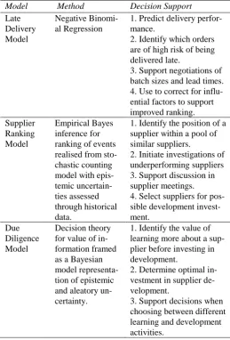
Table 1. Summary of modelling methods and decisions.

Model Method Decision Support

Late Delivery Model

Negative Binomi-al Regression

1. Predict delivery perfor-mance.

2. Identify which orders are of high risk of being delivered late.

3. Support negotiations of batch sizes and lead times. 4. Use to correct for influ-ential factors to support improved ranking. Supplier

Ranking Model

Empirical Bayes inference for ranking of events realised from sto-chastic counting model with epis-temic uncertain-ties assessed through historical data.

1. Identify the position of a supplier within a pool of similar suppliers.

2. Initiate investigations of underperforming suppliers 3. Support discussion in supplier meetings. 4. Select suppliers for pos-sible development invest-ment.

Due Diligence Model

Decision theory for value of in-formation framed as a Bayesian model representa-tion of epistemic and aleatory un-certainty.

1. Identify the value of learning more about a sup-plier before investing in development.

2. Determine optimal in-vestment in supplier de-velopment.

3. Support decisions when choosing between different learning and development activities.

2.2 Late delivery model

Late deliveries can cause severe impacts on produc-tion. Consequences can range from minor inconven-ience through to late penalty charges from the end customer. Delivery performance is a critical means for judging a supplier, but represents a highly com-plex relationship. It reflects not only the supplier, but the relationship between the supplier and manufac-turer and the manufacmanufac-turer’s ability to effectively manage the relationship. For manufacturers with global supply chains there are numerous variables believed to influence whether a delivery will arrive on time or be late. Consider the potential events which may cause a delivery to arrive late. Early in the relationship between a manufacturer and a sup-plier there may be issues associated with the inter-faces between the data management systems of ei-ther parties, or the manufacturer may be delayed in sending drawing specifications and so hold up pro-gress at the supplier. For the supplier, during produc-tion of parts, there may be machine failures, raw ma-terial problems, unanticipated rework, and scrappage due to newness of parts. During transportation of parts from supplier to manufacturer, a logistics com-pany may fail to pick up the part on time, shipment may be delayed due to weather, delays at customs may occur, and delays at goods received of the com-pany all may prevent items arriving on-time. For supply chain managers understanding the con-sequences of loading decisions is of key importance. Being able to formalise the relationships between, for example, production loading and delivery per-formance of a supplier is regarded as providing a useful tool. Understanding the associated degree of risk for different orders is required to allow supply managers to better formulate orders as well as to an-ticipate orders which are of high risk of arriving late. Data for delivery performance is recorded routine-ly in the manufacturing company and can be ob-tained from their enterprise planning system. Each record represents one delivery and contains associat-ed covariate information about the order, i.e. the number of parts ordered, lead time of part, supplier, date ordered, and so on. Naturally, for large manu-facturers there exists a large amount of records.

Given the nature of the target variable of interest (i.e. count of number of days or weeks a delivery is late), the suitability of count models are clear for this problem. Further, since we have a set of covariates driving lateness, as well as the large empirical data set that is constructed from delivery records, we adopt the well-established Negative Binomial re-gression modelling (Hilbe 2007) as the specific type of count model to predict lateness of orders. Count data has advantages in that it collapses the count of interest, in the context discussed here this is the late-ness of delivery which is measured as a non-negative integer value, and relates this to a set of covariates

(Hilbe 2007). Data for the covariates can also be taken from the enterprise resource planning system. 2.3 Supplier ranking model

Supply managers currently assess the relative per-formance of sets of suppliers, although this tends to be based upon simple statistical ratios. For example, late delivery rates given by the number of late deliv-eries relative to the number of orders for a given time window, or the non-conformance rate given by the number of non-conforming parts relative to the number of parts ordered for orders delivered over a given time horizon. However, as mentioned earlier, the patterns of orders and order sizes is highly varia-ble between different suppliers depending upon the nature of their part and also through time depending upon end customer orders. Methods are required that take into consideration this heterogeneity in the ex-posure of suppliers to risk.

We have developed an empirical Bayes method for ranking Poisson count data with heterogeneous exposure to risk; see Quigley et al. (in prep.a). Em-pirical Bayes is an established method of statistical inference and has been used in many risk and insur-ance applications especially where low frequency, or zero frequency events are the norm (e.g. Quigley et al. 2007). In our research, we have developed a nov-el means of ranking using empirical Bayes inference that allows us to compute point and interval esti-mates. The latter are particularly useful as they allow managers to distinguish between statistically differ-ent performances between suppliers. Interval esti-mates help us avoid the pitfalls of naïve over-interpretation of the rankings listed in a league table by allowing suppliers who are clearly in a class of their own to be differentiated from those that are in-distinguishable in terms of their performance.

2.4 Due diligence model

As well as taking decisions to maintain or to exit a relationship with an existing supplier with whom the manufacturer has empirical evidence of past perfor-mance, choices can be made about how much to in-vest in developing new suppliers in the interval be-tween their contract and first delivery. This interval may be of the order of several months and in some cases up to two years. For a new supplier evidence of anticipated performance will be based on data col-lected during the procurement process, including, for example, audits and parts production tests. Hence for all suppliers, new and established, evidence exists that allows uncertainties in performance to be articu-lated, although the nature of the data used and the degree of uncertainty may vary between suppliers. We propose a novel modelling approach to sup-port managers to decide the optimal level of invest-ment in supplier developinvest-ment under uncertainty about performance. This model is applicable for all suppliers. Further, we can provide managers with an assessment of the probability of gaining better per-formance by selecting a new supplier from the mar-ket rather than continuing to use an existing supplier. This can aid decisions concerned with exiting cur-rent suppliers, whether these choices are motivated by a poor supplier performance record or by pres-sures to switch to lower cost suppliers for which there will be uncertainty about performance.

We have developed a Poisson-Gamma probability model within a Bayesian framework, allowing us to represent both the epistemic (state-of-knowledge) and aleatory uncertainties in the event rates. Full mathematical details are given in Quigley et al. (in prep.b). Using this model we can obtain estimates to value a supplier development activity and to assess whether it is worth gaining more information, through, for example, further auditing, to reduce ep-istemic uncertainty. This model can be populated us-ing empirical data records on, for example, non-conformance frequencies to represent the aleatory uncertainty in the form of a Poisson counting pro-cess. The epistemic uncertainty in, say, the true non-conformance rate can be represented through the prior distribution. This prior distribution can be es-timated as an empirical prior using empirical Bayes inference if a suitable pool of suppliers can be se-lected and justified allowing their historical perfor-mance data to be used. Or, the prior distribution can be specified subjectively using methods of structured expert judgement. Other parameters required to pop-ulate the model include an assessment of the effec-tiveness of a supplier development activity as well as the financial value of lost production due to an unus-able or unavailunus-able part. Supply managers can be supported in expressing their judgements about the likely effectiveness of activities and sensitivity anal-ysis can be run to explore values across a range of effectiveness rate values. We have chosen to express

our model results as a function of the unit cost for lost production as this allows managers to insert val-ues for this unit costs and to scale up as appropriate. This also avoids requiring financially sensitive data to be required as a model input.

3 ANALYSIS OF SUPPLIER RISK 3.1 Overview

We now show a selection of analysis conducted us-ing de-sensitised data from a manufacturer that illus-trates the application of the modelling methods and discusses the choices made in data preparation. All analysis shown is “real” insofar as the supplier is-sues, the data and the results are based on an indus-try-based study. Note that the applications reported have only been undertaken after the methods them-selves (e.g. supplier ranking and due diligence mod-els) have been subject to extensive scientific evalua-tion theoretically and for simulated experiments. The analysis presented is a selection only and hence our examples draw upon different commodity groups and failure events to provide illustration.

3.2 Prediction of late deliveries

The data used are constructed from the delivery records for all suppliers in the commodity for a peri-od of one year. The variables which are available in the enterprise resource planning system are limited but new variables have been defined and constructed using existing records based on discussion with the supply chain managers. For example, covariates in-clude those capturing supplier loading such as order lines per week, number of parts ordered per week, whether order placed within the lead time and the nature of the logistics used to make delivery.

To give a sense of the data, historical perfor-mance data on the aspect of delivery failure is rec-orded individually. For each delivery received at the manufacturer, there is a record of the delivery. Each entry represents a delivery of a type of part. The en-try captures standard delivery details, including the supplier, the part type, lead time of the part, deliv-ered date and expected delivery date. Thus, we have records for every delivery made.

included. By comparing the observed count of late deliveries against the predicted count, Figure 2 shows that visually the model describes the actual performance variation well. It is apparent that the model oscillates between over- and under-predicting but there are no obvious discrepancies between pre-dicted and observed distributions.

Figure 2. Predicted and observed weeks late for commodity da-ta set under Negative Binomial regression model.

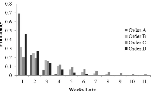
The model can be used to generate risk profiles for future order scenarios. Figure 3 compares the risk profiles of four order scenarios, labelled A-D. Each corresponds to different loading and logistic settings. The predicted probability distributions of number of late deliveries of different lengths of delay allow us to explore how different input scenarios are realised as risk profiles. Order scenario C decays slowest, showing more uncertainty and a relatively high chance of very late orders as indicated by the thick-est right tail. In contrast, order scenario A decays faster showing there is less chance of arriving late and has a lower expected mean number of days late. The results from such modelling can be presented visually as we have shown, but also numerically. Ei-ther way, the analysis allows the order characteristics to be examined before placing the order or prior to scheduled delivery so that action can be taken to avoid or at least mitigate the effects of late delivery on production.

3.3 Comparative assessment of suppliers

We show analysis for one commodity group com-prising 35 suppliers. Empirical data consists of his-torical delivery and non-conformance performance records which we have translated into counts of the number of late deliveries, numbers of orders, number of non-conformances and number of parts. For illus-tration we show analysis for overall performance of each supplier within one financial year. The methods of ranking can be applied to counts over any speci-fied time interval of interest to the managers. For ex-ample, the equivalent results can be obtained for counts of failure events over weekly, monthly, quar-terly or other time intervals and could also be updat-ed on a rolling basis since this type of analysis re-lates to regular operational management reviews. Figures 4 through 6 show different visual presen-tations of the data analysis. Figure 4 shows an ex-tract from a tabular display ranking the suppliers from best to worst performing in terms of late deliv-ery. The empirical Bayes (EB) late delivery rate is given for each supplier together with the raw data. The empirical Bayes delivery rate is a weighted av-erage of the estimated mean late delivery rate of the pool of 35 suppliers and the classical estimator of the late delivery rate for a given supplier. The mean rank and the 95% interval estimates for the mean rank can be computed. The point estimate of the mean rank naturally starts at 1 for the best perform-ing supplier on delivery and ends at 35 for the worst supplier. The range of the interval corresponds to the length of the bar. The width of the interval estimate can be interpreted as a statistical test to distinguish between those suppliers that are in class of their own (i.e. upper - lower = 0) or whether there are sub-sets of suppliers with similar performance and so “equiv-alent” ranks (i.e. upper – lower limit > 0). For exam-ple, in terms of late delivery performance, supplier S4 is the best, and suppliers S5, S18, S6, S10, S22, S2 are second best and statistically performing around the same level given that we adjust for their different exposures to risk. In contrast, supplier S35 is worst, S20 is second worst and S31 is third worst, while S11, S33, S32 are fourth worst.

Figure 5 shows boxplots of the distribution of ranks for the 35 suppliers for both late delivery and non-conformance. This visual shows the distribution of ranks, where the mean rank is denoted by a dia-mond and the quartiles by the box, with lines out to the minimum and maximum values. The mean ranks are those given numerically in column 4 of Figure 4. The boxplots provide information about the ex-pected ranks as well as the variation in the distribu-tion. The suppliers are given on the horizontal axis according to their supplier code (i.e. S1, S2,…, S35). For example, consider supplier S4 whose distribu-tions for both late deliveries and non-conformances indicate less variation than with, say, supplier 34 based on relative spreads of the distributions. Com-Figure 3. Predicted later delivery risk profiles under four

parison between the boxplots indicates that supplier S4 performs well on delivery given the mean and median rank position, but is one of the worst five suppliers in terms of non-conformance and so part quality. Hence, we can gain insight into the uncer-tainty about performance from the spread of the dis-tributions of ranks, we assess the positioning of a supplier relative to peers for a particular perfor-mance measure and we can compare perforperfor-mance across multiple measures for a given supplier.

Figure 6 shows the relationship between the mean rank of late deliveries against the mean rank of non-conformances for the pool of 35 suppliers. The im-mediate impression is of no clear pattern of relation-ship given the scatter of points, each representing a

supplier position. However, it is possible to identify the overall best and worst performing suppliers since these will be in the bottom left and top right of the scatter plot given we have defined rank = 1 to be the best. In this data set, supplier S6 is performing well in terms of delivery and quality performance, while the Pareto optimal set of suppliers S11, S32, S20 and S35 are performing poorly on both aspects of per-formance. Thus the supply managers have infor-mation about where to target effort to develop and also where lessons can be learnt from good suppliers through benchmarking.

3.4 Due diligence model

For suppliers identified as performing poorly the de-cision of whether to exit the supplier or to invest in them through a development activity must be made. Let us show how we may conduct such analysis by focussing on quality performance.

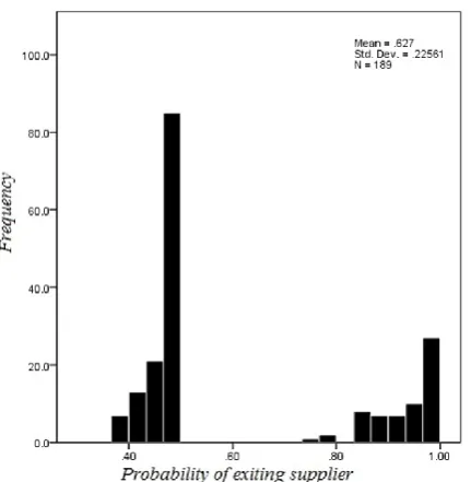
Figure 7 shows the probability of improving per-formance with respect to non-conper-formance by re-placing a supplier with a random selection from the market for a pool of 200 suppliers across multiple commodity groups. Two clusters of suppliers emerge. Taking 0.5 as natural division, there are a substantial number of suppliers with probabilities less than a 0.5 implying that these are not candidates for exit, but for development. There are around 60 suppliers for which it is more likely that the market will give a better supplier if performance remains at current levels since their probabilities exceed 0.5. A supply manager can determine an appropriate cut-off level with respect to the probability and determine a level which if a supplier is below triggers a flag for possible exit, meaning the supplier would not be contracted for future projects, or for development.

Figure 8 shows the prior distributions of the epis-temic uncertainty in the true non-conformance rate Figure 5. Box plots of distribution of ranks for late

deliver-ies (LD) and non-conformance (NC) for supplier pool.

Figure 6. Scatter plot of mean late delivery rank against mean non-conformance rank for pool of 35 suppliers, with Pareto frontiers (top right = worst, bottom left = best). Figure 4. Extract of late delivery ranks from best to worst

for a supplier of interest and of one randomly chosen from the market and so without any history with the manufacturer. As we gain experience with a suppli-er, over time the uncertainty will decrease, as depict-ed with the supplier of interest having much smaller variability. The question is, how much is it worth in-vesting to reduce our epistemic uncertainty about the supplier of interest by conducting developing activi-ties to learn more about their performance capabili-ties? That is, to reduce the variation of the prior dis-tribution. Also, should we invest to learn more or should we simply decide whether or not to directly invest in development activities?

Figure 9 shows a simple decision box that provides a visual representation to help answer these questions. The vertical axis represents the prior distribution for the true non-conformance rate and the horizontal ax-is represents the ratio of the added cost-benefit of a development activity, which is a function of the fi-nancial value of lost production, the effectiveness rate of an activity to learn or develop a supplier, and the anticipated reduction (or removal) of epistemic uncertainty due to supplier development. The scaling is such that the 450 line represents the decision rule that distinguishes between situations where it is worth investing and those where investment in sup-plier development would not be the optimal strategy. For example, in Figure 9, the prior mean of the sup-plier with the dashed distribution of epistemic uncer-tainty covers both grey and black zones and as such it may or may not be cost-effective to develop, so would be worth learning more about before deciding on whether to develop. The supplier represented by the solid line falls in the black zone and hence im-plies that learning more about this supplier will not change the decision, i.e. it is not worth investing in supplier development.

4 IMPLICATIONS AND CONCLUSIONS

The extracts from analysis presented has evolved through a longitudinal study with a manufacturer of bespoke variants of engineering systems assembled using parts sourced from a complex, global supply chain. By engaging over a period of two years, we have had continuous opportunity to learn more about the related issues that concern the supply managers, their desire to have evidence to support and chal-lenge their experience, their relative trust in empiri-cal data and their awareness of the under-utilisation of the information contained in operations databases. We have adopted an iterative approach to defining model purpose, developing methods with different degrees of scientific novelty, and evaluating applica-Figure 9. Decision box to support assessment of relative added cost-benefit of supplier development under different prior epis-temic uncertainty of true non-conformance rate.

tions within trial contexts using data from multiple commodity sets of suppliers over time horizons spanning several months to several years. To date, relatively more industry feedback has been gained through application of the late delivery prediction model and the supplier performance compared with the due diligence model. All models have been sub-ject to scientific validation, reported elsewhere, but all also require to be subject to further industry vali-dation. In summary, we consider our impact to date to be as follows.

We have shown how empirical records in data-bases and enterprise resource planning systems orig-inally collected for operations management, can be exploited to provide insights to better understanding of patterns and causal factors to help manage risk.

We have been able to provide statistical evidence through modelling that has been directly relevant to on-going supply management tasks, such as supplier performance ranking and late delivery predictions. The visual forms of evidence presentation has un-dergone several iterations, and will continue to be re-fined as we continue to learn about useful ways of presenting mathematical modelling in visual and management friendly ways.

We have scoped a road-map for analysis of sup-ply risk that is grounded in a coherent probability modelling framework and includes different model-ling purposes that align with decisions made at dif-ferent stages in the life of the supplier relationship with the manufacturer. Our models have been popu-lated with variables for which data, empirical and judgemental, are available. Although the general na-ture of the underlying methods allows for the inclu-sion of other variables, that are currently acknowl-edged as possibly influencing supply risk but have not been directly observable so far. We are consider-ing ways of measurconsider-ing such variables to increase the predictive capability of the late delivery model.

We have explored how forming appropriate pools of suppliers can support better inference and hence assessment of risk. This challenges the conception that suppliers should be pooled according to part type or commodity group only, which while useful for other reasons is not necessarily the most appro-priate for probabilistic analysis of risk. Although not shown, we can for example adjust the pools of sup-pliers to compensate for factors that statistically in-fluence performance through regression modelling.

We have gained a degree of acceptance by supply managers that their state of knowledge (epistemic) uncertainties can be represented in models as prior distributions, although to date we have mainly used empirical priors. Another piece of ongoing work re-lates to the elicitation of epistemic uncertainties.

We have developed algorithms to support compu-tational implementation of the methods in spread-sheets, which is the default general-purpose analysis tool in the manufacturing companies. Our initial

analysis has been conducted with more specialised software, such as the R package for the Negative Bi-nomial regression analysis and Maple for the suppli-er ranking and due diligence models. Exact infsuppli-erence can be mathematically challenging and computation-ally expensive in some instances. Hence research work has been undertaken to create and verify algo-rithms and approximations to validate them so that our models can be easily applied by practitioners.

Our future work will span industry validation studies of the methods developed and trialled to date and scientific research to extend modelling to in-clude decision models that capture suppliers, as well as the manufacturer, perspectives to inform strategic supply management decisions under uncertainty.

More generally, the methods presented have been explained and used in the context of supply risk management. However, the modelling methods are general and so can be used for risk analysis in other contexts where counts of events require to be mod-elled to support comparative performance analysis of different entities and estimating the value of invest-ing to improve performance and reduce risk.

REFERENCES

Hilbe, J.M. 2007. Negative binomial regression. Cambridge: Cambridge University Press.

Gallien, J., Mersereau, A., Novoa, M., Dapena, A., Garro, A. (2015). Initial shipment decisions for new products in Zara. Operations Research, Vol. 63.2, pp.269-286.

Quigley J., Bedford, T., Walls L. (2007). Using empirical Bayes to estimate the rate of occurrence of rare events. Re-liability Engineering and System Safety, Vol. 92, pp.619-627.

Quigley, J., Walls, L., Parsa. M. (in prep.a). A ranking method for Poisson count data with heterogeneous exposure: appli-cation to operational supply risk management.

Quigley, J., Walls, L., Demirel, G., Maccarthy, B., Parsa, M. (in prep.b). Is it worth developing a supplier? The value of information under uncertainty. European Journal of Opera-tional Research.

Sohdi, M.S. and Tang, C.S. (2012). Managing supply chain risk, Springer.

ACKNOWLEGEMENTS