The all-loop integrable spin-chain for strings on AdS3 × S 3 × T 4: The massive sector

      

City, University of London Institutional Repository

Citation

:

Borsato, R., Sax, O. O., Sfondrini, A., Stefanski, B. and Torrielli, A. (2013). The all-loop integrable spin-chain for strings on AdS3 × S 3 × T 4: The massive sector. Journal of High Energy Physics, 2013(8), doi: 10.1007/JHEP08(2013)043

This is the unspecified version of the paper.

This version of the publication may differ from the final published

version.

Permanent repository link:

http://openaccess.city.ac.uk/2776/

Link to published version

:

http://dx.doi.org/10.1007/JHEP08(2013)043

Copyright and reuse:

City Research Online aims to make research

outputs of City, University of London available to a wider audience.

Copyright and Moral Rights remain with the author(s) and/or copyright

holders. URLs from City Research Online may be freely distributed and

linked to.

arXiv:1303.5995v2 [hep-th] 3 May 2013

ITP-UU-13/08 SPIN-13/05 DMUS-MP-13/08

The all-loop integrable spin-chain for strings on

AdS

3

×

S

3

×

T

4

: the massive sector

Riccardo Borsato

1

, Olof Ohlsson Sax

1

, Alessandro Sfondrini

1

,

Bogdan Stefa´

nski, jr.

2

and Alessandro Torrielli

3

1. Institute for Theoretical Physics and Spinoza Institute, Utrecht University, Leuvenlaan 4, 3584 CE Utrecht, The Netherlands

2. Centre for Mathematical Science, City University London, Northampton Square, EC1V 0HB London, UK

3. Department of Mathematics, University of Surrey, Guildford, GU2 7XH, UK

R.Borsato@uu.nl, O.E.OlssonSax@uu.nl, A.Sfondrini@uu.nl, Bogdan.Stefanski.1@city.ac.uk, a.torrielli@surrey.ac.uk

Abstract

We bootstrap the all-loop dynamic S-matrix for the homogeneouspsu(1,1_|2)2 spin-chain believed to correspond to the discretization of the massive modes of string theory on AdS3 ×S3×T4. The S-matrix is the tensor product of two copies of

1

Introduction

The AdS/CFT correspondence [1] is a remarkable framework for relating quantum gauge and gravity theories. In certain, often highly (super-)symmetric settings, underlying the duality is an integrable structure.1 _{The presence of integrability gives a powerful tool}

for finding the mass spectrum of all perturbative states in the gauge/gravity dual pair in the planar limit. Initially, integrability was best understood in the case of N = 4 super-Yang-Mills (SYM) and its type IIB string dual on AdS5×S5 supported by RR fluxes, as

well as its orbifolds, orientifolds and deformations. Later, the integrability approach was extended to the so-called ABJM super-Chern-Simons theory and its type IIA string dual on AdS4×CP3. This provided a second class of examples of a gauge/string dual pair in

which the spectral problem is very well understood. The AdS4/CFT3 dual pair has less

supersymmetry than the original AdS5/CFT4,2 and has a number of new features, such

as Chern-Simons gauge fields, as well as scalars that transform in the bifundamental representation of the gauge group. It is a remarkable fact that much of the integrability machinery could be extended to this setting too.

Another interesting instance of the correspondence is the case of AdS3/CFT2, which

constitutes one of the earliest examples of holography, where the conformal symmetry algebra is infinite dimensional [3]. The maximally supersymmetric string backgrounds are AdS3 ×S3 ×T4 and AdS3 ×S3 ×S3×S1, both preserving 16 supercharges. Both

backgrounds can be supported by RR or NSNS fluxes. In the particular case of pure NSNS background it was possible to effectively describe the theories using the NSR formalism [4]. The CFT corresponding to the former background is expected to be a deformation of the SymN_(T4_{) orbifold theory, and have small N = (4,4)}

superconfor-mal symmetry [5]; the one corresponding to AdS3×S3×S3×S1 has large N = (4,4)

superconformal symmetry but is much less well understood [6]. Their finite dimensional sub-algebras are psu(1,1_|2)2 _{and d(2,1;α)}2 _{respectively, corresponding to the}

superi-sometries of each background.

The success of integrability in the more supersymmetric instances sparked new in-terest in the AdS3/CFT2 correspondence. Even if integrability in the CFT side remains

challenging [7], it has been shown that the RR string non-linear sigma model is clas-sically integrable [8, 9].3 _{As a result, one can make progress by discretising the string}

world-sheet and reducing the integrable system to a set of Bethe Ansatz equations [8, 11]. However, this procedure keeps track only of the excitations which remain massive in the BMN limit. Fully incorporating the massless modes remains an open issue.4

At weak coupling the Bethe equations yield the spectrum of an integrable spin-chain. The symmetry algebra preserving the vacuum of the spin-chain can be extended by three central charges [13, 8] and so one may attempt to construct an S-matrix generalising the bootstrap method presented in [14] for the S-matrix of fundamental particles of the AdS5/CFT4 correspondence. In [15], this approach was applied to the alternating

spin-chain related to string theory on AdS3×S3×S3×S1 constructed in [11], yielding a set

1_{For a recent review and an extensive list of references see [2].}

2_{The AdS}

5/CFT4and AdS4/CFT3 dual pairs have 32 and 24 real supercharges, respectively. 3_{This was later extended to backgrounds supported by a mixture of NSNS and RR fluxes, see [10].}

of all-loop Bethe equations [16].

One may be tempted to consider the AdS3×S3×T4 background as a limiting case

of the AdS3 × S3 ×S3 × S1 one, where one of the spheres blows up. While this is

certainly true for the gauge fixed string Hamiltonian, such a limit (which amounts to sendingα_→1) is quite subtle at the level of the symmetry algebra, of its representations, and therefore of the invariant S-matrix. In particular, the notion of fundamental and composite excitations is different in the two cases, so that one cannot simply send α_→1 in the S-matrix and Bethe ansatz of [15, 16]. Instead, one should repeat the bootstrap procedure from scratch for the psu(1,1|2)2 _{chain of [11]. This is the main aim of this}

work.

This paper is organised as follows. First, in section 2 we review thepsu(1,1_|2)2_chain,

discuss the symmetry algebra of its vacuum, and its central extension. Out of these symmetries we write down the all-loop S-matrix in section 3, where we also show that it solves the Yang-Baxter equation; the S-matrix is fixed up to two antisymmetric scalar factors, which we constrain by imposing crossing symmetry. In section 4 we diagonalise the S-matrix, write down the resulting Bethe ansatz, which describes the massive sector of the corresponding string theory, and discuss its weak and strong coupling limits. Finally, in section 5 we compare our results with perturbative calculations appeared in the literature, and section 6 is devoted to some concluding remarks. In appendix A we work out the dualities of the Bethe ansatz we found, and in the following two appendices we discuss how integrability for the AdS3/CFT2 correspondence can be framed in the

context of Hopf algebras and Yangians.

2

The

psu(1

,

1

|

2)

2

symmetric spin-chain

In this section we will review the psu(1,1|2)2 _{homogeneous spin-chain originally}

con-structed in [11]. The two copies of the superalgebra psu(1,1|2) describe the left- and right-moving sectors of string theory in AdS3 ×S3 ×T4. The weak coupling limit of

this spin-chain was analysed in [11]. In this limit, the left- and right-movers decouple. The spectrum is then described by two homogeneous spin-chains with the sites of each transforming in the representation (₋1

2; 1

2) ofpsu(1,1|2). At higher loops the two sectors

couple to each other through local interactions. The full spin-chain will be discussed in more detail below.

The algebra. The superalgebra psu(1,1_|2) has, in the relevant real form, a bosonic subalgebra sl(2)⊗su(2). The corresponding generators are denoted by S0,S± and L5, L±, respectively. Additionally, there are eight supercharges Q±±±. The commutation

relations of psu(1,1_|2) algebra read

[S0,S±] =±S±, [S+,S−] = 2S0, [S0,Q±ββ˙] =±

1

2Q±ββ˙, [S±,Q∓ββ˙] =Q±ββ˙, [L5,L±] =±L±, [L+,L−] = 2L5, [L5,Qb±β˙] =±

1

{Q±++,Q±−−}=±S±, {Q±+−,Q±−+}=∓S±, {Q+±±,Q−∓∓}=−S0±L5,

{Q+±+,Q−±−}=∓L±, {Q+±−,Q−±+}=±L±, {Q+±∓,Q−∓±}= +S0∓L5.

(2.1)

The psu(1,1|2) algebra admits au(1) automorphism generated byR8 and acting on the

supercharges as5

[R8,Qbβ±] =±

1

2Qbβ±, (2.2)

and commuting with the bosonic charges.

The full symmetry of the spin-chain is psu(1,1|2)×psu(1,1|2). When we need to distinguish the left- and right-moving copies of the algebra we will add an additional subscript, taking values L and R, to the generators.

Serre-Chevalley bases. For superalgebras there are in general several inequivalent Dynkin diagrams, corresponding to different choices of simple roots. Each such choice corresponds to a set of Cartan generators hi, and corresponding raising and lowering

operators ei and fi, where the index i takes values from 1 to the rank of the algebra,

which is 3 for psu(1,1|2). These generators satisfy an algebra of the form

[hi,hj] = 0, [ei,fj] =δijhj, [hi,ej] = +Aijej, [hi,fj] =−Aijfj, (2.3)

where Aij is the Cartan matrix.

In this paper we will mainly consider two gradings ofpsu(1,1_|2). In thesu(2) grading the simple roots are given by

h1 =₋S0₋L5, e1 = +Q+−−, f1 = +Q−++, h2 = +2L5, e2 = +L+, f2 = +L−, h3 =−S0−L5, e3 = +Q+−+, f3 =−Q−+−.

(2.4)

This leads to the Cartan matrix

  

0 −1 0

−1 +2 ₋1 0 ₋1 0

 

. (2.5)

The corresponding Dynkin diagram is shown in figure 1 (a). In the sl(2) grading we have

ˆ

h1 = +S0+L5, ˆe1 =₋Q−++, ˆf1 = +Q+−−,

ˆ

h2 =−2S0, ˆe2 = +S+, ˆf2 =−S−,

ˆ

h3 = +S0+L5, ˆe3 =−Q−+−, ˆf3 =−Q+−+,

(2.6)

with the Cartan matrix _

 

0 +1 0 +1 −2 +1

0 +1 0

 

. (2.7)

5_{We denote the automorphism byR}

+1

(a)

±1

(b)

−1

[image:6.595.104.516.488.625.2]

(c)

Figure 1: Three Dynkin diagrams forpsu(1,1|2).

The Dynkin diagram for the sl(2) grading is shown in figure 1 (c).

There are also fermionic gradings of psu(1,1_|2), in which all three raising operators

ei are odd. In particular we can choose them to be either

Q+−+, Q++−, Q−++, or Q−+−, Q−−+, Q+−−.

This leads to the Cartan matrices

  

0 +1 0 +1 0 ₋1

0 −1 0

 

, and

  

0 −1 0

−1 0 +1 0 +1 0

 

, (2.8)

respectively, corresponding to the Dynkin diagram in figure 1 (b).

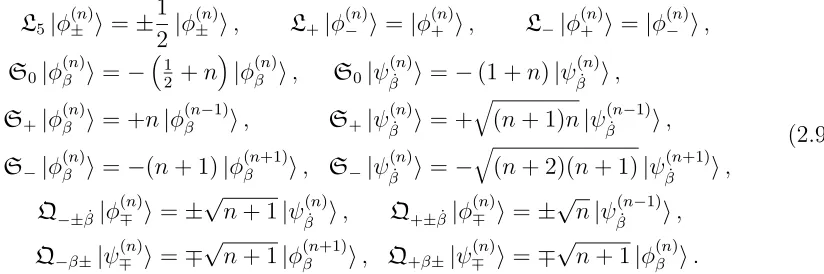
The spin-chain representation. The sites of thepsu(1,1_|2) spin-chain transform in the infinite dimensional representation (−1

2; 1

2), consisting of the bosonic su(2) doublet φ±(n) and the two fermionic su(2) singlets ψ±(n), where the index n indicates the sl(2)

quantum number. The action of the generators on these states is given by

L5|φ(±n)i=±

1 2|φ

(n)

± i, L+|φ(−n)i=|φ (n)

+ i, L−|φ(+n)i=|φ (n) − i,

S0|φ(βn)i=−

1 2 +n

|φ(_βn)_i, S0|ψ_β(˙n)i=−(1 +n)|ψ (n)

˙

β i,

S+|φ(βn)i= +n|φ

(n−1)

β i, S+|ψ_β(˙n)i= +

q

(n+ 1)n_|ψ_β(_˙n−1)_i,

S−|φ(βn)i=−(n+ 1)|φ

(n+1)

β i, S−|ψ_β(˙n)i=−

q

(n+ 2)(n+ 1)|ψ_β(˙n+1)i,

Q_−±β˙|φ(∓n)i=±

√

n+ 1_|ψ(_β˙n)_i, Q_+±β˙|φ(∓n)i=±

√

n_|ψ(_β˙n−1)_i,

Q−β±|ψ∓(n)i=∓

√

n+ 1|φ(_βn+1)i, Q+β±|ψ∓(n)i=∓

√

n+ 1|φ(_βn)i.

(2.9)

The highest weight state _|φ(0)+ i is annihilated by the su(2) grading raising operators Q+±±, as well as by the two generators Q−+±. Hence, the representation (−1₂;1₂) is a

short representation, satisfying the shortening conditions

The ground state. The states of the left- and right-moving spin-chains of length6 _L

transform in theL-fold tensor product of the above representation. The ground state of the full spin-chain is given by

|0_iL =(φ(0)+ )L

E

⊗(φ(0)+ )L

E

. (2.11)

This is the highest weight state of the short 1/2-BPS representation (−L

2;

L

2)⊗(−

L

2;

L

2)

of psu(1,1|2)×psu(1,1|2). In each sector this state is constructed from the spin-chain module discussed above. Hence, the ground state is preserved by eight supercharges QI

i

and SI

i, with i= 1,2 and I =L, R, as well as two central charges H

I

, which in terms of the psu(1,1|2) generators are given by

QI

1 = +Q I

−++, Q I

2 =−Q I

−+−, S I

1 = +Q I

+−−, S I

2 = +Q I +−+, HI

=−SI 0−L

I 5,

(2.12)

This forms two psu(1|1)2_{⋉u(1) algebras}

{QI

i,S

J

j}=δijδIJHI. (2.13)

The charges HL

and HR

are the left- and right-moving spin-chain Hamiltonians. It is useful to introduce the combinations

H=HL

+HR

, M=HL

−HR

. (2.14)

The HamiltonianH gives the energy of a spin-chain state, and depends on the momenta of the spin-chain excitations. The central charge Mmeasures the angular momentum in AdS3 and should be independent of the spin-chain momentum.

We can introduce two additionally generators B1 and B2 acting as outer

automor-phisms on the above algebra. These can be constructed from the psu(1,1_|2) generators

LI

5 and the automorphisms RI8,

B1 =−(R

L

8−R

R

8)−(L

L

5−L

R

5), B2 = +(R

L

8−R

R

8)−(L

L

5−L

R

5). (2.15)

The above linear combinations are chosen so that B1 commutes with QI2 and SI2, while B2 commutes with QI1 and SI1. The commutation relations involving the supercharges

then read

[Bi,Q

L

j] =−δijQ

L

i, [Bi,S

L

j] = +δijS

L

i,

[Bi,Q

R

j] = +δijQ

R

i, [Bi,S

R

j] =−δijS

R

i.

(2.16)

Taking the generatorsBi into account it is useful to regroup the symmetry algebra into

two copies of u(1)⋉su(1|1)2_{, with the generators given by}

n

QL

1,S

L

1,Q

R

1,S

R

1,H

L

,HR

,B1

o

, and nQL

2,S

L

2,Q

R

2,S

R

2,H

L

,HR

,B2

o

, (2.17)

respectively. Since the central charges HL

and HR

are shared between the two su(1_|1)2

algebras, the full symmetry preserving the ground state can be written as

h

u(1)⋉_psu(1|1)2i2⋉_u(1)2_{. (2.18)} 6_{The symbol L is used to denote the length and to denote left-moving generators and excitations.}

|φ(0)_{− i}

|ψ(0)₊ i − |ψ(0)₋ i

|φ(1)₊ i +Q1

+S1

+Q1

+S1

+Q2

+S2

[image:8.595.244.353.101.202.2]

−Q2 −S2

Figure 2: The action of the superchargesQiandSion the bi-fundamental representation (2.19).

Excitations. To construct excited spin-chain states we replace one or more of the ground state sites by any other state in the same module. We can classify these excita-tions by their eigenvalues under the left- and right-moving spin-chain Hamiltonians HL

andHR at zero coupling. Let us consider excitations in the left-moving sector. Replacing

one of the highest weight states φ(0)+ by the scalar φ−(n) orφ(+n) increases the eigenvalue of HL

by n or n+ 1, respectively. Similarly, insertion of a fermion ψ±(n) also adds n to the

energy. The lightest excitations are therefore

φ(0)− , ψ (0)

+ , ψ (0)

− , and φ

(1) + .

These states form a four-dimensional bi-fundamental representation of the left-moving

psu(1_|1)2 _{algebra (2.13), as illustrated in figure 2. To emphasize this we introduce the}

notation

Φ+ ˙+ = +φ(0)− , Φ− ˙

− _{= +φ}(1)

+ , Φ− ˙

+ _{= +ψ}(0)

+ , Φ+ ˙− =−ψ (0)

− . (2.19)

We also introduce the symbolsǫγ and ǫγ˙ to keep track of the grading

(₋1)ǫ± ₌

±1, (₋1)ǫ±˙ =±1. (2.20)

The excitation Φγγ˙ _{then has statistics (−1)}ǫγ+ǫγ˙_.

To make the bi-fundamental nature of the representation above more explicit, we introduce an auxiliary fundamental su(1_|1) representation with basis (φ_|ψ), and the generators Q, Sand Hacting as

Q_|φi=a|ψi, S_|ψi=b|φi, H_|φi=ab|φi, H_|ψi=ab|ψi. (2.21)

We can then identify

Φ+ ˙+=φ⊗φ, Φ+ ˙− =φ⊗ψ, Φ−+˙ =ψ⊗φ, Φ−−˙ =ψ⊗ψ. (2.22)

The supercharges QL

1 and S

L

1 only act on the first index of Φγγ˙, while Q

L

2 and S

L

2 act on

the second index. Hence the action on the tensor products (2.22) is given by

QL

1 =Q⊗1, S

L

1 =S⊗1, Q

L

2 = 1⊗Q, S

L

Note that we get a minus sign from commuting a supercharge through a fermion when we act with the charges of the second type on a state with a fermion in the first part of the tensor product. Hence, the left-moving generators act as

QL

1|Φ+ ˙+i= +a|Φ− ˙ +

i, QL

1|Φ+ ˙−i= +a|Φ− ˙ −

i, SL

1|Φ− ˙

+_{i= +b|Φ}+ ˙+_{i, S}L

1|Φ− ˙

−_{i= +b|Φ}+ ˙−_i,

QL

2|Φ+ ˙+i= +a|Φ+ ˙−i, Q

L

2|Φ− ˙

+_i=−a|Φ−−˙_i,

SL

2|Φ+ ˙−i= +b|Φ+ ˙+i, S

L

2|Φ− ˙

−_i=−b|Φ−+˙_i,

(2.24)

with the right-moving charges acting trivially. Comparing the above representation with (2.9) we find that the central charge HL

has eigenvalue ab= 1.

Similarly, we introduce the right-moving excitations ¯Φ±±˙_{, transforming in a}

bi-fundamental representation of the right-moving psu(1_|1)2 _algebra.

The centrally extended algebra. When we take quantum corrections into account, the spin-chain HamiltonianHshould depend on the coupling constant and on the momen-tum of the excitations. This requires the bi-fundamental representations discussed above to be deformed. However, this should be done in such a way that the angular momentum

M remains undeformed. This means that we need to consider a generalized symmetry algebra in which the right-moving generators act nontrivially on the left-moving exci-tations, and vice versa. Hence, we introduce two additional central charges P and P†

appearing in the anti-commutator between a left- and a right-moving supercharge

{QL

i,Q

R

j}=δijP, {S

L

i,S

R

j}=δijP†. (2.25)

Exactly like the central charges HL

and HR

, these charges are shared between the two copies of u(1)⋉_su(1|1)2_{. Hence, the extended algebra can be written as}7

h

u(1)⋉_psu(1|1)2i2⋉_u(1)4_{. (2.26)}

This is the maximal central extension of psu(1_|1)4_.

Since the charges in general are momentum dependent we will consider spin-chain states in which the excitations carry specific momenta. A one-excitation state can then be written as a plane wave

|Xpi=

L

X

n=1

eipn_|Zn−1_XZL−n_{i, (2.27)}

where X is any left- or right-moving excitation, and we have introduced the shorthand notation Z for a ground-state site. It is now straightforward to generalize this form to the case of multiple excitations. Note that we always consider asymptotic states, where

7_{The role of the central extensions for psu(1}

|1)2 _{was originally discussed in [17], in the context of}

the spin-chain is considered to be very long and the excitations are well separated. The interactions are then described by the S-matrix permuting the order of excitations along the chain.

In order to construct nontrivial representations of the extended algebra we need to allow the supercharges to have a length-changing action on the spin-chain excitations. We therefore introduce two additional symbolsZ± _{indicating the insertion or removal of}

a vacuum site next to an excitation. Writing out the plane waves we can commute these symbols through an excitation of momentum pby picking up an extra phase factor

|Z±Φβ_pβ˙i=e∓ip|Φβ_pβ˙Z±i (2.28)

Using these relations we can always shift any insertions of Z± _{through all excitations}

and collect them at the right end of the state.

A centrally extended su(1_|1)2 _{algebra with dynamic spin-chain representations was}

considered in [15]. The supercharges act on the left-moving excitations by

QL

|φpi=ap|ψpi, Q

L

|ψpi= 0,

SL

|φpi= 0, SL

|ψpi=bp|φpi,

QR

|φpi= 0, QR

|ψpi=cp|φpZ+i,

SR

|φpi=dp|ψpZ−i, S

R

|ψpi= 0.

(2.29)

The left-moving charges in the above expressions act in the same way as in (2.21). Hence, the bi-fundamental representations in (2.24) can be deformed to a representation of the centrally extended algebra (2.26) by considering a tensor product of the representation (2.29). We find that the left-moving generators act on the left-movers Φ±±˙ _{in the same}

way as in (2.24), but with the coefficients a and b depending on the momentum of the excitation. The action of the right-moving supercharges is given by

QR

1|Φ− ˙ −

p i= +cp|Φ+ ˙p−Z+i, Q

R

1|Φ− ˙ +

p i= +cp|Φ+ ˙p+Z+i,

SR

1|Φ+ ˙p+i= +dp|Φ−p+˙Z−i, S

R

1|Φ+ ˙p−i= +dp|Φ−p−˙Z−i,

QR

2|Φ− ˙ −

p i=−cp|Φp−+˙Z+i, Q

R

2|Φ+ ˙p−i= +cp|Φ+ ˙p+Z+i,

SR

2|Φ+ ˙p+i= +dp|Φ+ ˙p−Z−i, S

R

2|Φ− ˙ +

p i=−dp|Φ−p−˙Z−i.

(2.30)

Closure of the algebra requires the central charges to act on the left-movers as

HL

|Φ±p±˙i=apbp|Φ±p±˙i, P|Φ±

˙ ±

p i=apcp|Φ±p±˙Z+i,

HR

|Φ±_p±˙i=cpdp|Φ±p±˙i, P†|Φ±

˙ ±

p i=bpdp|Φ±p±˙Z−i.

(2.31)

The central chargesPandP† _{are not part of the symmetries of thepsu(1,1|2)}2

spin-chain. They therefore need to vanish on a physical state. Acting with Pon a spin-chain state with two left-moving excitations, we obtain

P_|Φβ_pβ˙Φγ_qγ˙_i= (e−iqapcp+aqcq)|Φβ

˙

β

p Φγqγ˙i. (2.32)

Setting

we find

e−iqapcp+aqcq=h(e−i(p+q)−1), (2.34)

which vanishes provided the excitations satisfy the momentum constraint ei(p+q) _{= 1.}

Similarly, requiring the charge P† to vanish on a physical state leads us to

bpdp =h(e+ip−1), (2.35)

We furthermore require that the generator M remains undeformed when the central excitations are turned on, which gives

apbp−cpdp = 1. (2.36)

The above conditions on the coefficients of the representation together uniquely deter-mines the dispersion relation

E(p) =apbp+cpdp =

r

1 + 16h2_sin2 p

2. (2.37)

To write down the explicit form of the coefficients ap, . . . , dp it is useful to introduce

the spectral parameters x± _{satisfying [14]}

x+

p

x−

p

=eip, x+_p + 1

x+

p

!

− x−_p + 1

x−

p

!

= i

h. (2.38)

The coefficients can then be written as

ap = + √

h ηp, bp = + √

h ηp, cp =− √

hiηp x+

p

, dp = + √

hiηp x−

p

, (2.39)

where

ηp =

q

i(x−

p −x+p). (2.40)

The above expressions are essentially the same as those given in [15], apart from a rescaling of the coupling constant h by a factor 2 and setting the parameter s labeling the representations there to s= 1 as appropriate in AdS3×S3×T4.

The right-movers again transform in a similar representation in which the roles of the left- and right-moving generators have been interchanged.

3

S-matrix

In order to derive the S-matrix_Sfor the excitations discussed above we will follow closely the procedure of [15]. We focus on the two-particle S-matrix,

|Yq(out)Xp(out)i=S |Xp(in)Yq(in)i. (3.1)

where S acts on the spin-chain state by permuting the excitations. First of all, we require that _S commutes with the whole centrally extended symmetry algebra, i.e., for any generatorJ

Furthermore, the S-matrix should satisfy the unitarity condition

S12S12 =1, (3.3)

and physical unitarity, which means that the S-matrix should be unitary as a matrix, so that if S _{is the matrix form of S on a basis of asymptotic two-particle states, we have}

S_{pq ·(}S_pq)† _{= (}S_pq)†_·S_{pq =1⊗1. (3.4)}

On top of this we will also require that there is aZ2 left-right symmetry, so that matrix elements that differ by interchanging left and right chiralities should be equal.

In this way we find two solutions, corresponding topure transmissionandpure reflec-tion of the “left” and “right” flavors. Consistence with the string theory results [20, 21] forces us to choose the pure transmission S-matrix, like in [15]. The similarity with those results is not accidental, and in fact much deeper, since the excitations of thepsu(1,1|2)2

chain transform under two copies of the centrally extended su(1_|1)2 _{algebra discussed}

in [15]. In fact this makes the whole S-matrix factorize into two copies of the su(1|1)2

invariant one,

S =_Ssu(1|1)2⊗ Sˆ _su(1|1)2, (3.5)

where the hat denotes a graded tensor product, so that in components we have

Skl_{mn ≡}SKK,L˙ L˙

MM ,N˙ N˙ = (−1)

ǫM˙ǫN+ǫK˙ǫL_S su(1|1)2

KL M N

S_su(1|1)2

_M˙_L˙ ˙

MN˙ , (3.6)

where the ǫ symbol is 0 for bosons and 1 for fermions. This tensor product structure is very similar to the one coming from the centrally extendedpsu(2|2)×psu(2|2) symmetry of [14].

It is convenient to rewrite here the explicit form of Ssu(1|1)2, in a slightly different

normalization with respect to [15]. We have

Ssu(1|1)2|φ_pφ_qi= ALL_pq|φ_qφ_pi, S_su(1|1)2|φ_pψ_qi= B_pqLL|ψ_qφ_pi+C_pqLL|φ_qψ_pi,

Ssu(1|1)2|ψ_pψqi= F_pqLL|ψ_qψpi, S_su(1|1)2|ψ_pφ_qi=DLL_pq|φ_qψ_pi+E_pqLL|ψ_qφ_pi,

(3.7)

where the coefficients take the form

ALL

pq =Spq, B

LL

pq =Spq

x+

q −x+p

x+

q −x−p

, CLL

pq =Spq

x+

q −x−q

x+

q −x−p

ηp

ηq

,

FLL

pq =−Spq

x−

q −x+p

x+

q −x−p

, DLL

pq =Spq

x−

q −x−p

x+

q −x−p

, ELL

pq =Spq

x+

p −x−p

x+

q −x−p

ηq

ηp

,

(3.8)

and Spq is an antisymmetric phase that cannot be fixed by symmetries and unitarity

alone. Then we have, e.g.,

S |Φ+ ˙_p+Φ+ ˙_q+_i=ALL

pqA

LL

pq|Φ+ ˙q+Φ+ ˙p+i, S |Φ+ ˙_p+Φ−_q−˙_i=BLL

pqB

LL

pq |Φ−

˙ −

q Φ+ ˙p+i+C

LL

pqC

LL

pq |Φ+ ˙q+Φ−

˙ −

p i

+BLL

pqC

LL

pq

|Φ−_q+˙Φ+ ˙_p−i − |Φ+ ˙_q−Φ−_p+˙i,

and so on.

In the LR-sector the scattering is reflectionless and we have

Ssu(1|1)2|φ_pφ¯_qi=ALR_pq |φ¯_qφ_pi+BLR_pq |ψ¯_qψ_pZ−i, S_su(1|1)2|φ_pψ¯_qi=C_pqLR|ψ¯_qφ_pi,

Ssu(1|1)2|ψ_pψ¯qi=E_pqLR|ψ¯_qψpi+F_pqLR|φ¯_qφ_pZ+i, S_su(1|1)2|ψ_pφ¯_qi=D_pqLR|φ¯_qψ_pi.

(3.10)

We normalize the S-matrix so that the elements are

ALR

pq = +τ

LR

pq

1_{− x}+1

px

−

q

1₋ 1

x−px

−

q

, BLR

pq =−τ

LR

pq

ηpηq

x−

px−q

1 1₋ 1

x−px

−

q

, CLR

pq =τ

LR

pq,

ELR

pq =−τ

LR

pq

1₋ 1

x−px+q

1− 1

x−px

−

q

, FLR

pq =−τ

LR

pq

ηpηq

x+

px+q

1 1− 1

x−px

−

q

, DLR

pq =τ

LR

pq

1₋ 1

x+px+q

1− 1

x−px

− q . (3.11) where τLR

pq =ζpqSepq, ζpq =

v u u u t1−

1

x−px−q

1− 1

x+px+q

, (3.12)

and Sepq is an undetermined antisymmetric phase. Using (3.5) it is easy to work out the

scattering in the LR-sector of the psu(1,1_|2)2 _{chain, finding,e.g.,}

S |Φ+ ˙_p+Φ¯+ ˙_q+_i=ALR

pqA

LR

pq |Φ¯+ ˙q+Φ+ ˙p+i −B

LR

pqB

LR

pq |Φ¯−

˙ −

q Φ−

˙ −

p Z−Z−i

+ALR

pqB

LR

pq

|Φ¯+ ˙_q−Φ+ ˙_p−Z−i+|Φ¯−_q+˙Φ−_p+˙Z−i,

S |Φ+ ˙_p+Φ¯−_q−˙_i=CLR

pqC

LR

pq |Φ¯−

˙ −

q Φ+ ˙p+i,

(3.13)

where we explicitly wrote down the length-changing effects.

Due to the discrete LR-symmetry, the S-matrix in the RL and RR sectors can be easily found from the previous expressions, again just like in [15]. Due to this symmetry, the only unknown scalar factors in the S-matrix are Spq and Sepq.

An early attempt of deriving the S-matrix for the AdS3 ×S3 ×T4 massive modes

was made in [22]. However, there the interaction between left- and right-moving sectors was not analyzed in full detail, and as a result the S-matrix contained only one dressing phase.

More recently another proposal was made for the AdS3×S3×T4 S-matrix [23]. This

has not used the central extensions we discussed in section 2 above. The resulting S-matrix and Bethe ansatz therefore differ from the ones presented here, in particular in the LR-sector.

3.1

The Yang-Baxter equation

For an integrable theory, an N-body scattering process can be broken down into a se-quence of two-body scattering events. The condition that ensures that this can be done in a consistent way is the Yang-Baxter equation, which amounts to requiring that the two ways in which a 3-body scattering can be decomposed are equivalent. In terms of the operator _S this reads

where we recall that _S permutes the excitations.

Our S-matrix satisfies the Yang-Baxter equation (3.14). However, to check this we must not forget that in our spin-chain picture S may add or remove vacuum sites after a two particle excitiation, as in (3.13). If we want to rewrite the Yang-Baxter equation on a basis of asymptotic excitations, we must take into account these vacuum sites by shifting them to the far right of the spin chain, as explained in section 2. This results in additional factors ofe±ip_{wherepis the momentum of the rightmost excitation. Therefore}

the Yang-Baxter equation reads, in matrix form,

1⊗S_{pq ·} F_qS_prF_q−1_{⊗1· 1⊗}S_{qr =}F_pS_qrF−_p1_{⊗1 · 1⊗}S_{pr ·} F_rS_pqF−_r1_{⊗1, (3.15)}

where the transformation F _{implements a twist depending on the momentum of the}

third excitation. It is convenient to introduce a new S-matrix Sb _{that, unlike}S_{, obeys the}

untwisted Yang-Baxter equation [24, 15]

1⊗Sb_{pq ·} Sb_{pr ⊗1 · 1⊗}Sb_{qr =}Sb_{qr⊗1 · 1⊗}Sb_{pr ·} bS_{pq ⊗1. (3.16)}

This can be done by means of a nonlocal transformation on the two-particle basis in terms of a twist operator U_{(p) defined as}

b

S_{pq =}U†_{(p)⊗1 ·} S_{pq ·} U_{(q)⊗1. (3.17)}

The factor F_{p in (3.15) is then related to}U_{(p) by}

F_{p =}U_(p)⊗U_{(p). (3.18)}

More specifically, if we let our one-particle basis be given by

Φ+ ˙+_,Φ+ ˙−_{, Φ}−+˙_,Φ−−˙_,Φ¯+ ˙+_{, Φ¯}+ ˙−_,Φ¯−+˙_{, Φ¯}−−˙_{, (3.19)}

the operator U_{(p) is given by}8

U_{(p) = diage}−i p_{, e}−i p/2_{, e}−i p/2_{, 1, e}−i p_{, e}−i p/2_{, e}−i p/2_{,1. (3.20)}

It is now easy to check that our spin chain S-matrixS_{satisfies (3.15) or equivalently that}

b

S_{, which is sometimes called the “string frame” S-matrix, satisfies (3.16). This points to}

the integrability of the underlying theory.

3.2

Crossing symmetry

The integrable S-matrix that we have found depends on two undetermined antisym-metric phases Spq and Sepq, which we now want to constrain. One way to do so is, as

in [15], to exploit the fact that there exists two-particle configurations (“singlets”) that are annihilated by the whole symmetry algebra,

J _|1pqi= 0. (3.21)

8_{We have fixed the twist matrix by requiring that also in the string frame it is true that bS =}

b

This feature was first noticed for AdS5 strings [14] and also there it can be employed to

find constraints on the S-matrix [25, 26]. In fact, since _|1pqi is completely neutral, its

scattering with any excitation should be trivial (see equation (3.24) below). This yields a constraint on the product of pairs of S-matrix elements. Furthermore, since_|1pqi should

have zero energy, it follows that either p or q cannot be physical. In fact it turns out that they must be related by crossing, that is in term of the Zhukovski variables

x±(p) =x±(¯q) = 1

x±_(q). (3.22)

As discussed in [25] for AdS5 strings, it is indeed possible to relate the triviality of

scattering by a singlet with the requirement of crossing symmetry. In what follows we will obtain the crossing equations for Spq and Sepq first by considering the scattering of

a singlet with an arbitrary excitation, and later by requiring crossing invariance for the (string frame) S-matrix.

Solving (3.21) yields two singlets, related to each other by LR-symmetry. These can be constructed by tensoring two copies of singlet discussed in [15]. They are9

|1LRpp¯ i=|Φp+ ˙¯+Φ¯+ ˙p+Z+Z+i+ Ξpp¯ |Φ−p¯+˙Φ¯− ˙ +

p Z+i+ Ξpp¯ |Φp+ ˙¯−Φ¯+ ˙p−Z+i −(Ξpp¯ )2|Φ−p¯−˙Φ¯− ˙ −

p i, |1RLpp¯ i=|Φ¯+ ˙p¯+Φ+ ˙p+Z+Z+i+ Ξpp¯ |Φ¯−p¯+˙Φ−

˙ +

p Z+i+ Ξpp¯ |Φ¯+ ˙p¯−Φp+ ˙¯−Z+i −(Ξpp¯ )2|Φ¯−p¯−˙Φ− ˙ −

p i,

where

Ξpp¯ =i x+p

η¯p

ηp

, x±_p¯ = 1

x±

p

. (3.23)

Requiring that the scattering with any excitation _|Xpi is trivial

S23S12|Xp1LRqq¯ i=|1LRqq¯ Xpi, S23S12|Xp1RLqq¯ i=|1RLqq¯ Xpi, (3.24)

gives the crossing equations.

In order for the S-matrices to have the standard su(2) andsl(2) form we rewrite the scalar factors as

S_pq−2 = x

+

p −x−q

x−

p −x+q

1_{− x}+1

px

−

q

1₋ 1

x−

px+q

σ2_pq, Se_pq−2 = 1−

1

x+px

−

q

1₋ 1

x−

px+q

e

σ_pq2 , (3.25)

where σ2

pq and σe2pq are two new phases, which we will refer to as the “dressing phases”.10

9_{In what follows we write them taking the momenta p, q to be in the physical region. Crossing is}

indicated by ¯p,q¯, which corresponds to a shift on the rapidity torus by half of its imaginary period [27]. Antisymmetry requires shift in the first and second variable to be performed in opposite directions, see appendix B, which leaves us with two seemingly equivalent prescriptions. The preferred choice can be fixed by comparing perturbative results with the dressing phases that solve the crossing equations [28].

10_{The appearance of two independent dressing phase factors was previously observed in [18] for the}

They satisfy the crossing equations

σ_pq2 σe_p2_q¯= x

+

p

x−

p

!2

(x−

p −x+q)2

(x−

p −x−q)(x+p −x+q)

1− 1

x−px+q

1₋ 1

x+px

−

q ,

σ_p2_q¯σe_pq2 = x

+ p x− p !2

1_{− x}−1

px

−

q 1− 1

x+px+q

1_{− x}+1

px

−

q

2

x−

p −x+q

x+

p −x−q

.

(3.26)

It is easy to check that, in both the finite-gap and near-BMN limits, these equations are satisfied if we take both phases to be equal to the AFS one [29] at leading order,

σ(p, q) = σAF S(p, q) +O

₁

h2

, σe(p, q) =σAF S(p, q) +O

₁

h2

, (3.27)

where

σAF S(xp, xq) =

 1−

1

x−px+q

1− 1

x+px

−

q

 

 1−

1

x+px

−

q

1− 1

x+px+q

1₋ 1

x−px+q

1− 1

x−px

−

q

 

ih(xp+1/xp−xq−1/xq)

. (3.28)

We plan to discuss an all-loop solution to these crossing equations in an upcoming publication [28].

The same set of equations can be found also by the usual field-theoretic consider-ations [25]. It is convenient to work in the string frame, and for this purpose let us transform the charges of the symmetry algebra as

b

J_{pq =}U†_q⊗1·J_pq·U_{q⊗1, (3.29)}

whereJ_{pq is the matrix representation of the generator}Jon a two-particle state andJb_{pq is}

its string frame counterpart. Then the action on a two-particle states can be understood in terms of a nontrivial coproduct

ˆ

J_{pq =}J_p⊗e±i q/2_{+ Σ⊗}J_{q, (3.30)}

where one should pick the positive sign in the exponent for the supercharges SI

i and the

negative one for QI

i, and Σ takes into account the fermion signs. In particular, in the

basis (3.19), we have

Σ = diag ( 1,−1,−1, 1, 1,−1,−1, 1). (3.31)

By taking the supertranspose of the charges J _{we find another representation related to}

the original one by charge conjugation as

C−1_·J_(z+ω)st_{·C =−e}∓i p/2J_{(z), (3.32)}

where C is the charge conjugation matrix which in our basis reads11

C = 0 −i

i 0 ! ⊗     

1 0 0 0

0 −1 0 0 0 0 ₋1 0 0 0 0 ₋1

   

. (3.33)

11_{There are more general solutions to (3.32). We fixed our choice by pickingC}

·C† _{= C}†

·C = 1

To simplify our notation it is useful to rewrite the S-matrix in terms of an operator that does not permute the excitations. To this end we introduce

R_{pq = Π·}S_{pq, (3.34)}

where Π is the permutation matrix. In terms of R_{pq the fundamental invariance}

prop-erty (3.2) becomes

R_pq·J_p⊗e±iq/2 _{+ Σ⊗}J_q=J_{p⊗Σ +e}±ip/2_⊗J_q·R_{pq. (3.35)}

We can now follow a standard route [25] to derive the crossing equations for R_{pq, taking}

the transpose of (3.35) with respect to either factor of the tensor product, and exploiting the charge conjugation (3.32).12 _{The crossing equations then read}

C−1⊗1·Rt1

¯

qp·C⊗1·Rqp=1⊗1, 1⊗C−1·Rtp2q¯·1⊗C·Rpq =1⊗1, (3.36)

where the superscript t1,2 denotes transposition in the first or second factor, or

ΣC−1_⊗1·Rt1

¯

qp·CΣ⊗1·Rqp=1⊗1, 1⊗ΣC−1·Rtp2q¯·1⊗CΣ·Rpq =1⊗1, (3.37)

depending on whether we shift down or up the first variable of the S-matrix under crossing, see footnote 9. We can take e.g. the second equation in (3.36) and evaluate it in terms of the S-matrix elements in the string frame finding that it is satisfied if, e.g.,

ApqAepq¯= 1, Bpq¯Cepq = 1, (3.38)

where

Apq =hΦ+ ˙_q+Φ+ ˙_p+|Sb_pq|Φ+ ˙_p+_Φ+ ˙_q+_{i, Apq}e _=hΦ¯+ ˙_q+_Φ+ ˙_p+_|Sb_pq|Φ+ ˙_p+_Φ¯+ ˙_q+_i,

Bpq =hΦ−_q−˙Φ+ ˙_p+|Sb_pq|Φ+ ˙_p+_Φ−_q−˙_{i, Cpq}e _=hΦ¯−_q−˙_Φ+ ˙_p+_|Sb_pq|Φ+ ˙_p+_Φ¯−_q−˙_i. (3.39)

Using the explicit form of the S-matrix elements yields (3.26). The first equation in (3.36) gives similar equations where the crossed momentum is in the first argument of the S-matrix; these can also be found from considering scattering with a singlet, but with a particle incoming from the right.

Let us remark that, up to a different choice of normalization, the crossing equations are the square of the ones found in [15] for _Ssu(1|1)2, see also appendix B. In section 4.4

we will discuss the solutions at strong coupling of these crossing equations and further constraints on the scalar factors.

It is also interesting to notice that the action of the charges on the two-particle states (3.30) takes the form of a nontrivial coproduct, similar to the one appearing in other instances of AdS/CFT integrability [30, 31]. This suggests an alternative route to obtain the all-loop S-matrix: rather than bootstrapping it out of its symmetries, and obtaining an integrable S-matrix as a result, we could have postulated the existence of an underlying Hopf algebra structure. This is yet another route to obtain the crossing equations (3.26), which we discuss in appendix B. Furthermore, and in contrast with what happens in the case of AdS5, here we could have in principle obtained the whole

S-matrix from a universal R-matrix (the one of gl(1|1)) by imposing Yangian symmetry. We refer the reader to appendix C for details on this construction.

12_{To this end it is useful to rewrite (3.32) asJ(z)}t₌

−e±ip/2_C

·J(z₋ω)_·C−1

4

S-matrix diagonalisation and Bethe ansatz

Since the all-loop S-matrix_Spq obtained in the previous section satisfies the Yang-Baxter

equation, we can use it to obtain the asymptotic Bethe ansatz for the spin chain.

4.1

Diagonalising the S-matrix

In this section we show how to construct asymptotic eigenstates of the spin-chain Hamil-tonian H. We will follow closely the procedure used in [16] to diagonalise the S-matrix of the d(2,1;α)2 _{spin-chain. This procedure is standard [32, 14, 33, 34] and we will only}

present the key steps.

We will construct asymptotic eigenstates (i.e. eigenstates for a chain of infinite length) out of the two-particle S-matrix. One such eigenstate containing K excitations will be of the form

|Ψi= X

π∈SK

Sπ|ΨiI, Sπ = Y

(k,l)∈π

Skl, (4.1)

where π _∈ SK is a permutation, |ΨiI is a wavefunction and we used the fact that the

scattering factorizes to write the K-body S-matrix as a product of two-body ones, which act by

Sπ|Ψi=Sπ|Ψiπ. (4.2)

Since not all of the quantum numbers scatter by pure transmission we need to employ the so-called nesting procedure to perform the diagonalisation.

The idea is to introduce a level-I vacuum |0iI, which is just given by |ZL_{i. Then,}

rather than considering all of its possible excitations at once, we restrict to the maximal set of excitations that scatter diagonally. This will give the level-II vacuum _|0_iII. The remaining fields are then considered as level-II excitations on top of such a vacuum. This will be enough to diagonalise the whole S-matrix in our case.

Level-I vacuum. The level-I vacuum is just _|0_iI _{≡ |}ZL_{i. The S-matrixS given in the}

previous section can be thought of as the level-I S-matrix, and we will call it _SI _{in this}

section.

Level-II vacuum. We need to choose a maximal set of excitations that scatter with pure transmission among each other. An N-particle state made out of only this kind of excitations will be automatically an eigenstate. From the structure of SI _{leads to four}

possible choices

V_AII ={Φ+ ˙+,Φ¯−−˙}, V_BII ={Φ−−˙,Φ¯+ ˙+}, VII

C ={Φ+ ˙−,Φ¯−

˙

+_{}, V}II

D ={Φ−

˙

+_,Φ¯+ ˙−_}. (4.3)

Each candidate level-II vacuum is composed of one left and one right excitation, that are either both bosonic or both fermionic.

In the following we will choose the set VII

A to construct the level-II vacuum. In

QL

1 Q

L

2 S

R

1 S

R

2

Φ+ ˙+ _Φ−+˙ _Φ+ ˙− _Φ−+˙_Z− _Φ+ ˙−_Z−

¯

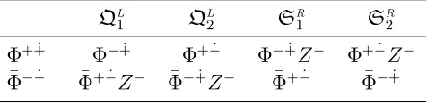
[image:19.595.180.418.98.157.2]

Φ−−˙ _Φ¯+ ˙−_Z− _Φ¯−+˙_Z− _Φ¯+ ˙− _Φ¯−+˙

Table 1: Action of the lowering operators on the states of the level-II vacuumVII

A.

Propagation. To consider also the other types of fields, we can view them as level-II excitations on the level-II vacuum. We have four supercharges at our disposal to create other types of fields, starting from the ones of VII

A (see table 1 for their explicit action).

Note that the fields Φ−−˙_,Φ¯+ ˙+ _{do not explicitly appear in the Bethe ansatz, since from}

that point of view they are considered as composite excitations (i.e., one can respectively create them by consecutively applying QL

1 and Q

L

2 on Φ+ ˙+ and S

R

1 and S

R

2 on ¯Φ− ˙ −_).

As in [16], we can derive the level-II S-matrix by requiring compatibility of the level-I S-matrix with the states in which we allow for one level-II excitation. In the following we consider two-particle states and we write the wave function that solves the compatibility condition with SI_{. The factorization of scattering allows us to extend these results to}

N-particle excitations, when one level-II excitation is allowed.

Starting from a level-II vacuum defined as|0iII22=|Φp+ ˙+Φ+ ˙q+i we can consider level-II

excitations created by the action of QL

1 as13

|YyiII(22) =f2(y, p)|Φ −+˙

p Φ+ ˙q+i+f2(y, q)S

II,I

22 (y, p)|Φ+ ˙p+Φ−

˙ +

q i, |YyiII(22),π =f2(y, q)|Φ

−+˙

q Φ+ ˙p+i+f2(y, p)S

II,I

22 (y, q)|Φ+ ˙q+Φ−

˙ +

p i.

(4.4)

The compatibility equation

SI

π|Yyi

II

(22) =A

LL

pqA

LL

pq|Yyi

II

(22),π (4.5)

is solved by

f2(y, p) =g2(y) ηp

h2(y)₋x+

p

, S22II,I(y, p) =

h2(y)₋x−

p

h2(y)₋x+

p

, (4.6)

where h1(y), g1(y) are arbitrary functions of y. Starting instead from a level-II vacuum defined as _|0_iII¯2¯2 = |Φ¯−

˙ −

p Φ¯−

˙ −

q i we can consider level-II excitations created by the action

of QL

1 as

|YyiII(¯2¯2) =f¯2(y, p)|Φ + ˙−

p Z+Φ−

˙ −

q i+f¯2(y, q)S_2¯¯II₂,I(y, p)|Φ− ˙ −

p Φ+ ˙q−i, |YyiII_(¯2¯2),π =f¯2(y, q)|Φ+ ˙q−Z+Φ−

˙ −

p i+f¯2(y, p)S_2¯¯II₂,I(y, q)|Φ− ˙ −

q Φ+ ˙p−i.

(4.7)

The compatibility equation

SπI|YyiII_(¯2¯2) =F

RR

pq F

RR

pq |YyiII_(¯2¯2),π (4.8)

13_{We use the index 2 when we consider level-II excitations on the field Φ}+ ˙+_{, while the index ¯2 for}

is solved by

f¯2(y, p) = − ig¯2(y)

x+

p

ηp

1₋ 1

h¯2(y) x

−

p

, S¯_2¯II₂,I(y, p) =

1_{− h} 1

¯ 2(y) x+p

1₋ 1

h¯2(y) x

−

p

. (4.9)

As beforeh¯2(y), g¯2(y) are generic functions ofy. The last step is to start from the level-II

vacuum _|0_iII_2¯2 =_|Φ+ ˙+

p Φ¯−

˙ −

q i. For the level-II excitation we can write

|YyiII(2¯2) =f2(y, p)|Φ −+˙

p Φ¯−

˙ −

q i+f¯2(y, q)S¯22II,I(y, p)|Φ + ˙+

p Φ¯+ ˙q−Z+i, |YyiII(2¯2),π =f¯2(y, q)|Φ¯q+ ˙−Z+Φ+ ˙p+i+f2(y, p)S

II,I

2¯2 (y, q)|Φ¯ −−˙

q Φ−

˙ +

p i.

(4.10)

and we can solve the equation

SπI|YyiII_(2¯2) =C

LR

pqC

LR

pq |YyiII_(2¯2),π (4.11)

by

h¯2(y) = h2(y)≡y, g¯2(y) =− g2(y)

h2(y),

S¯22II,I(y, p) = S II,I

22 (y, p), S2¯II2,I(y, p) =S II,I ¯

2¯2 (y, p).

(4.12)

These calculations are exactly equivalent to the ones already performed in [16]. This is not surprising, since in the diagonalisation procedure we have to consider doublets of

su(1_|1) (e.g. (Φ+ ˙+_|Φ−+˙_{) in the present case and (φ}1_|ψ1_{) in [16]). This makes clear that}

the diagonalisation procedure works in a similar way for the other level-II excitations.

Scattering. All the level-II excitations scatter trivially amongst each other. We show the explicit example in which we start from the level-II vacuum _|0_iII₂₂ = _|Φ+ ˙+

p Φ+ ˙q+i and

we create two level-II excitations by acting with the charge QL

1. The two-particle states

are

|Yy1Yy2i

II

(22) =f2(y1, p)f2(y2, q)S II,I

22 (y2, p)|Φ− ˙ +

p Φ−

˙ +

q i

+f2(y2, p)f2(y1, q)S₂₂II,I(y1, p)S₂₂II,II(y1, y2)_|Φ−_p+˙Φ−_q+˙_i,

|Yy1Yy2i

II

(22),π =f2(y1, q)f2(y2, p)S

II,I

22 (y2, q)|Φ− ˙ +

q Φ−

˙ +

p i

+f2(y2, q)f2(y1, p)S22II,I(y1, q)S22II,II(y1, y2)|Φ− ˙ +

q Φ−

˙ +

p i.

(4.13)

Requiring the equation

SI

π|Yy1Yy2i

II

(22) =A

LL

pqA

LL

pq|Yy1Yy2i

II

(22),π (4.14)

and using the previous results, we find that

S22II,II(y1, y2) =−1, (4.15)