Cross-Spectral Local Descriptors via Quadruplet Network

(1)

Cross-Spectral Local Descriptors via Quadruplet

Network

Cristhian A. Aguilera1,2,*, Angel D. Sappa1,3, Cristhian Aguilera4and Ricardo Toledo1,2

1 _{Computer Vision Center, Edifici O, Campus UAB, Bellaterra 08193, Barcelona, Spain;}

[email protected] (A.D.S.); [email protected] (R.T.)

2 _{Computer Science Department, Universitat Autònoma de Barcelona, Campus UAB, Bellaterra 08193,}

Barcelona, Spain

3 _{Facultad de Ingeniería en Electricidad y Computación, CIDIS, Escuela Superior Politécnica del Litoral,}

ESPOL, Campus Gustavo Galindo, Km 30.5 vía Perimetral, Guayaquil 09-01-5863, Ecuador

4 _{DIEE, University of Bío-Bío, Concepción 4051381, Concepción, Chile; [email protected]}

* Correspondence: [email protected]; Tel.: +56-9-30687318

Abstract: This paper presents a novel CNN-based architecture, referred to as Q-Net, to learn local feature descriptors that are useful for matching image patches from two different spectral bands. Given correctly matched and non-matching cross-spectral image pairs, a quadruplet network is trained to map input image patches to a common Euclidean space, regardless of the input spectral band. Our approach is inspired by the recent success of triplet networks in the visible spectrum, but adapted for cross-spectral scenarios, where for each matching pair there are always two possible non-matching patches; one for each spectrum. Experimental evaluations on a public cross-spectral VIS-NIR dataset shows that the proposed approach improves the state-of-the-art. Moreover, the proposed technique can also be used in mono-spectral settings, obtaining a similar performance to triplet network descriptors, but requiring less training data.

Keywords:cross-spectral; descriptor; infrared; CNN

1. Introduction

Over the last few years the number of consumer computer vision applications has increased dramatically. Today, computer vision solutions can be found in video game consoles [1], smartphone applications [2], and even in sports—just to name a few. Furthermore, safety-critical computer vision applications, such as autonomous driving systems, are not longer science fiction.

Ideally, we require the performance of those applications, particularly those that are safety-critical to remain constant under any external environment factor, such as changes in illumination or weather conditions. However, this is not always possible or very difficult to obtain solely using visible imagery, due to the inherent limitations of the images from that spectral band. For that reason, the use of images from different or multiple spectral bands is becoming more appealing. For example, the Microsoft Kinect 2 uses a near-infrared-camera to improve the detection performance in low light or no light conditions.

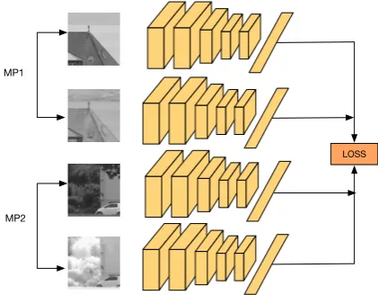
In this work we are particularly interested in cross-spectral applications, i.e., computer-vision applications that make use of two different spectral bands to provided a richer representation of a scene, that otherwise could not be obtained from just one spectral band. We present a novel CNN-based architecture, referred to as Q-Net, to learn local feature descriptors that are useful for matching image patches from two different spectral bands. Figure1 shows an illustration of our proposal. The training network consists of four copies of the same CNN, i.e., weights are shared, which accepts as input two different cross-spectral image matching pairs1. In the forward pass, the

1 _{A matching pair consists of two image patches that show the same scene, regardless of the spectral band of the patches.}

(2)

network computes severalL2 distances between the outputs of each CNN, obtaining the matching

pair with the biggestL2distance and the non-matching pair with the smallestL2distance that will be

later on used during the backpropagation step. This can be seen as always using the hardest cases of matching and non-matching pairs at each iteration. At testing, our network can be used as drop-in replacements for hand-made feature descriptors such as SIFT in various cross-spectral tasks such as stereo-vision, object detection and image registration. It is important to notice that during testing it is just necessary one of the four CNNs that were used during training. This CNN will act as a feature descriptor.

LOSS

MP1

MP2

Figure 1.The proposed network architecture. It consists of four copies of the same CNN that accepts

as input two different cross-spectral correctly matched image pairs (MP1 and MP2). The network

computes the loss based on multiplesL2 distance comparisons between the output of each CNN,

looking for the matching pair with biggestL2distance and the non-matching pair with the smallest

L2distance. Both cases are then used for backpropagation of the network. This can be seen as positive

and negative mining.

Our work is based on the recent success of the triplet network presented in [3], named PN-Net, but adapted to work with cross-spectral image pairs, where for each matching pair, there are two possible non-matching patches; one for each spectrum. Results show that our technique is useful for learning cross-spectral feature descriptors that can be used as drop-in replacements of SIFT-like features descriptors. Moreover, results also show that our network can be useful for learning local feature descriptors in the visible domain, with similar performance to PN-Net but requiring less training data.

In this article, we make the following contributions:

• We propose and evaluate three ways of using triplets for learning cross-spectral descriptors. Triplet networks were originally designed to work on visible imagery, so the performance on cross-spectral images is unknown.

• We propose a new training CNN-based architecture that outperforms the state-of-the-art in a public VIS-NIR cross-spectral image pair dataset. Additionally, our experiments show that our network is also useful for learning local feature descriptors in the visible domain.

• Fully trained networks and source code is publicly available athttp://github.com/ngunsu/ qnet.

(3)

(a) (b) (c)

Figure 2. VIS-NIR cross-spectral image pairs; top images are from the visible spectrum and bottom

images from the near-infrared spectrum

proposed technique, which are presented in section 4. Finally, in section 5 we show the validity of our proposal through several experiments, ending with the conclusions in section6.

2. Background and related work

This section briefly introduces the near-infrared spectral band and highlights similarities and differences between images from this spectrum with respect to the visible spectrum. Additionally, the VIS-NIR cross-spectral image dataset used as a case study through the different sections of this manuscript is also presented. Finally, the most important methods proposed in the literature to describe images from two different spectral bands are reviewed, together with current CNN-based descriptor approaches used to describe images in the visible spectrum.

2.1. Near-infrared band

The near-infrared band (NIR: 0.7-1.4µm) is one of the five sub-bands of the infrared spectrum (0.7-1000µm). It is the closest infrared sub-band to the visible spectrum and images from both spectral bands share several visual similarities; in Fig.2three pairs of VIS-NIR images are presented. It can be appreciated that images from both spectra are visually similar but with some notable differences. For example, red visible regions disappear in NIR images (see Fig.2(a)), the direction of the gradients can change (as in Fig.2(b)), and NIR images are more robust to different illumination settings (as in Fig.2(c)).

Recent advances in technology have made infrared imaging devices affordable for classical computer vision problems, from face recognition ([4]) to medical imaging ([5]). In some of these cases, infrared images are not used alone but in conjunction with images from other spectral bands (e.g., visible spectra). In these cases, infrared images need to be used in a framework that allows them to be handled in an efficient way in terms of the heterogeneity of the information ([6]), which is the main challenge to be solved and the motivation for current work.

2.2. Dataset

(4)

other half to non-matching pairs. Figure3 shows four samples of cross-spectral image pairs from the dataset.

(a) (b) (c) (d)

Figure 3. Image patches from the VIS-NIR training set. First row corresponds to grayscale images

from the visible spectrum; second row to NIR images. (a) and (b): non-matching pairs; (c) and (d): correctly matched pairs.

Table 1.Shows the number of cross-spectral image pairs per category on the VIS-NIR patch dataset

used to train and evaluate our work.

Category # Cross-spectral pairs

country 277504

field 240896

forest 376832

indoor 60672

mountain 151296

oldbuilding 101376

street 164608

urban 147712

water 143104

2.3. Cross-spectral descriptors

The description of two images from two different spectral bands in the same way is a challenging task that cannot always be solved with classical feature descriptors such as SIFT ([9]) or SURF ([10]), due to the non-linear intensity variations that may exist between images from two different spectral bands. Early efforts focused on modifying gradient-based descriptors to work between[0,π]instead of[0, 2π]to reduce the effect of changes in the gradient direction between images from two different spectral bands. For example, [11] and [12] applied this strategy to SIFT and HOG respectively, the first to match VIS-NIR local features and the second to compute the stereo disparity between a VIS and a thermal infrared camera. Although this strategy is simple, it improves the performance of those algorithms in cross-spectral scenarios.

(5)

rather than in image texture. In a similar way, [15] and [16] compute cross-spectral features using the EHD algorithm over the image patch response to different Log-Gabor filters.

In a more recent work, [7] tested different CNN-based networks to measure the similarity between images from the VIS-NIR and the VIS-LWIR spectra. In their experiments, they showed that CNN-based networks can outperform the state-of-the-art in terms of matching performance. However, with regard to speed, their networks are much slower than classical solutions, problem that we address in the current work, training a cross-spectral descriptor that can be used as a replacement of SIFT and many otherL2-based descriptors.

2.4. CNN-based feature descriptor approaches

During last decades carefullyhand-made feature descriptors, such as SIFT or SURF, have been popular in the computer vision community. However, in the last few years, such approaches have been started to be outperformed by CNN-based solutions in different feature descriptors benchmarks (e.g., [3,17,18]). [17] propose a max-margin criterion over a siamese network to compute the similarity between two different image patches. [18] follows a similar approach, but instead of using a metric network, it directly minimizes the L2 distance between the descriptor of two images in the loss

function, making their trained descriptor a drop-in replacement to SIFT-like descriptors. More importantly, it notices that after a few training epochs, most of the non-matching samples used to train the network were not giving new information, making it necessary to use mining strategies to improve the performance of the networks. In the same way, [3] propose a triplet network to mine negative samples with each input triplet, improving the performance of siamese networks.

The current works is strongly based on the triplet network proposed by [3], but adapted to be used in cross-spectral image pairs. We use quadruplet instead of triplet and we do not only mine non-matching samples but also correctly matched samples. In section3and4both architectures are detailed.

Notice that in this review, we only include CNN-based feature descriptors that can be used as a replacement for commonhand-madedescriptors, since they are useful for real-time applications. Other solutions have been proposed skipping the process of description and matching, doing everything with a CNN and trading matching performance for speed. For example, the 2ch network from [17], MatchNet from [19] and the siamese network from [20].

3. PN-Net (Triplet network)

In this section we describe the architecture of PN-Net ([3]); a state-of-the-art triplet network for learning local features descriptors. Although PN-Net was not intended to be used as a network for learning cross-spectral descriptors, we propose three ways to use PN-Net in such settings. In summary, this section objective is twofold:

• As previously stated, our network is similar to the triplet network but specifically designed to learn cross-spectral local feature descriptors. A brief description of this network will help to set the basis of our proposal in Section4.

• We explain the motivation behind our proposal through several experiments. After training PN-Net to learn cross-spectral feature descriptors, we discovered that the network performance improved when we randomly alternated between non-matching patches from both spectra.

3.1. PN-Net Architecture

(6)

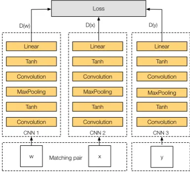
Finally, the output of eachtowerwill be a descriptorDof configurable size, that describes each input patch.

CNN 1 CNN 2 CNN 3

Convolution Tanh Linear

Convolution Tanh MaxPooling

Convolution Tanh MaxPooling Loss

Matching pair

D(w) D(x) D(y)

w x y

Figure 4.PN-Net training triplet architecture

3.2. PN-Net Loss

The loss function is described as follows:

Pm= e

∆+

emin(∆−1,∆−2)+e∆+

(1)

Pnm = e min(∆−

1,∆2−)

emin(∆−1,∆

−

2)+e∆+

(2)

Loss(Ti) =Pm2+ (Pnm−1)2 (3)

where, ∆+ corresponds to the L2 distance between the descriptors of the matching pair wand x,

||D(w),D(x)||2;∆−₁ corresponds to theL2distance between the descriptors of the non-matching pair

wandy,||D(w),D(y)||2; and∆−₂ corresponds to theL2distance between the descriptors of the second

non-matching pairxandy,||D(x),D(y)||₂.

In essence, the objective of the loss function is to penalize small L2 distances between

non-matching pairs, and largeL2distances between matching pairs. Ideally, we wantPmto be equal

to zero andPnm to be equal to one, i.e,∆+ <<min(∆−₁,∆−₂). Computing the minimumL2distances

between the non-matching pairs is a type of mining strategy, were the network always performs backpropagation using the hardest non-matching sample of each triplet T, i.e, the non-matching sample with the smallestL2distance. The mining strategy is used to avoid the problems described

in [18] and mentioned in section2. Finally, the MSE is used to penalize values ofPmdifferent of zero

and values ofPnmdifferent of one.

3.3. Cross-spectral PN-Net

(7)

Table 2.Average FPR95 for each category

Train seq. PN-Net Gray PN-Net NIR PN-Net Random

Country 11.79 11.63 10.65

Field 17.84 16.56 16.10

Forest 36.00 32.47 32.19

Indoor 48.21 47.26 46.48

Mountain 29.35 26.29 25.67

Oldbuilding 29.22 27.25 27.69

Street 18.23 16.71 16.73

Urban 32.78 36.61 33.35

Water 18.16 17.76 15.84

Average 26.84 25.84 25.08

We test each one of the aforementioned solutions in the dataset used in [7] and presented in section 2 . We train each network nine times, once per category and tested on the other eight categories. In Table 2, we present our results in terms of the false positive rate at 95% Recall (FPR95). In essence, we evaluate how well the descriptors can distinguish between correct and incorrect matches. Results show that randomly usingy between an NIR and RGB patch was better than the other two solutions. This give us a hint, that using images from both spectra to mine the network is better than using just from one, which we expected assuming that a balanced number of non-matching images from both spectra will help to produce better results.

CNN 1 CNN 2

Loss

Matching pair

D(w) D(x)

CNN 3 CNN 4

Matching pair

D(y) D(z)

w x y z

Non-matching pairs

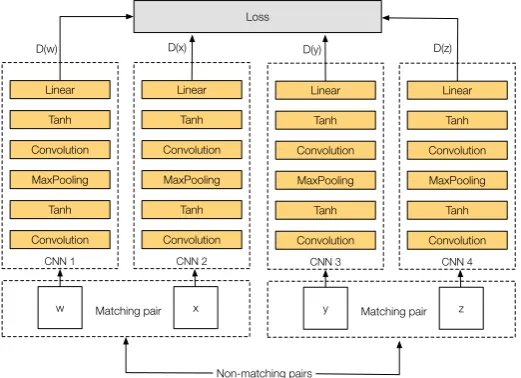
Figure 5.Q-Net training quadruplet architecture

4. Q-Net

(8)

4.1. Q-Net Architecture

The architecture of Q-Net is similar to PN-Net, but using four copies of the same network instead of three (see Figure5). The input is a tupleQ, with four different input patchesQ={w,x,y,z}, that is formed by two different cross-spectral matching pairs: (w, x), and (y, z), allowing the network to mine not just non-matching cross-spectral image pairs at each iteration, but also cross-spectral correctly matched pairs.

4.2. Q-Net Loss

Q-Net loss function extends the mining strategy from PN-Net presented in section 3.2. Specifically, we add two more distance comparisons toPnm, making the loss suitable for cross-spectral

scenarios, and we extend the mining strategy from the non-matching pairs to the correctly matched pairs. At each training step, the network uses the matching pair with larger L2 distance and the

non-matching pair with the smallestL2distance. The loss function is described as follows:

Pm= e

max(∆+₁,∆+₂)

emin(∆−1,∆−2,∆−3,∆−4)+emax(∆

+

1,∆

+

2)

(4)

Pnm = e

min(∆−

1,∆−2,∆3−,∆4−)

emin(∆−1,∆

−

2,∆

−

3,∆

−

4)+emax(∆

+

1,∆

+

2)

(5)

Loss(Qi) =Pm2 + (Pnm−1)2 (6)

where, ∆+₁ corresponds to the L2 distance between the descriptors of the matching pair wand x,

||D(w),D(x)||2; ∆+₂ corresponds to the L2distance between the descriptors of the matching pairy

andz,||D(y),D(z)||2;∆−₁ corresponds to theL2distance between the descriptors of the non-matching

pair w and y, ||D(w),D(y)||2; ∆−2 corresponds to the L2 distance between the descriptors of the

non-matching pairxandy,||D(x),D(y)||2;∆3−corresponds to theL2distance between the descriptors

of the non-matching pairwandz,||D(w),D(z)||2; and∆−₄ corresponds to the L2distance between

the descriptors of the non-matching pairxandz,||D(x),D(z)||2.

The proposed loss function takes into account all the possible non-matching combinations. For example, if we want to train a network to learn similarities between the VIS and the NIR spectral bands,Pnm will compare two VIS-NIR non-matching pairs, one VIS-VIS non-matching pair and one

NIR-NIR non-matching pair; instead of using a random function as we did with PN-Net. Moreover, since we are trying to learn a common representation between the NIR and the VIS, comparing VIS-VIS and NIR-NIR cases helps the network to have more training examples. Since it is necessary to have two cross-spectral matching pairs to computePnm, it was natural to extend the mining strategy

toPm, obtaining at each step the cross-spectral matching pair with the largerL2distance.

Our method allows to learn cross-spectral distances, mining positives and negatives samples at the same time. This approach can also be used in monospectral scenarios, providing a more efficient mining strategy than previous works. Results that support our claim are presented in the next section. More importantly, our method can be extended to other cross-spectral or cross-modality scenarios. Even more, it can be extended to other applications such as heterogeneous face recognition, where it is necessary to learn distance metrics between faces from different spectral bands.

5. Experimental evaluation

(9)

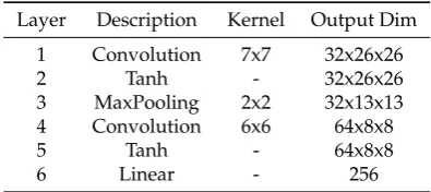
Table 3.Q-Net layer descriptions

Layer Description Kernel Output Dim

1 Convolution 7x7 32x26x26

2 Tanh - 32x26x26

3 MaxPooling 2x2 32x13x13

4 Convolution 6x6 64x8x8

5 Tanh - 64x8x8

6 Linear - 256

5.1. VIS-NIR scene dataset

In this section we evaluate the performance of our network on the VIS-NIR dataset presented in Section2. As in [7], we train on the country sequence and test in the remaining eight categories.

Training: Q-Net and PN-Net networks were trained using Stochastic Gradient Descent (SGD) with a learning rate of 1.1, weight decay of 0.0001, batch size of 128, momentum of 0.9 and learning rate decay of 0.000001. Trained data was shuffled at the beginning of each epoch and each input patch was normalized to its mean intensity. The trained data was split into two, where 95% of the data was used as training data and 5% as validation. Training was performed with and without data augmentation (DA), were the augmented data was obtained by flipping the images vertically and horizontally, and rotating the images by 90, 180 and 270 degrees. Each network was trained ten times to account for randomization effects in the initialization. Lastly, we used a grid search strategy to find the best parameters.

Model details: Model details are described in Table3. The layers and parameters are the same from [3], which after several experimental results showed to be suitable for describing cross-spectral patches. Notice that for feature description shallow models are suitable, since lower layers are more general than the upper ones.

Software and hardware:All the code was implemented using the Torch framework ([22]). The GPU consisted of an NVIDIA Titan X and the network was trained in between five and ten hours when we used data augmentation.

Results are shown in Table4. Firstly, we evaluated EHD ([14]) and LGHD ([16]), twohand-made descriptors that were used as a baseline in terms of matching performance. The performance of LGHD is under 10% and can be considered as state-of-art results—before the current work. Secondly, we test a siamese L2 network based on the work of [17] that performs better than EHD, but worst

than the state-of-art. Thirdly, PN-Net and its variant were tested, not being able to surpass the performance of LGHD without using data augmentation. On the other case, Q-Net showed to be better than the state-of-art even without data augmentation, showing the importance of mining on the non-matching and matching samples in cross-spectral scenarios. Additionally, we tested our model increasing the training data using the previously detailed data augmentation technique, improving the state-of-the-art by a 2.91%. For a more detailed comparison of the different feature descriptors evaluated in the current work, we provide the corresponding ROC curves in Fig.7.

In addition, we tested the performance when different descriptor sizes were used. Fig.6shows the results of our experiment. From the figure we can see that there is a gain in increasing the descriptor size until 256. Descriptor sizes bigger than 256 did not perform better.

5.2. Multi-view stereo correspondence dataset

Although the proposed approach has been motivated to tackle the cross-spectral problem, in this section we evaluate the proposed architecture when a visible spectrum dataset is considered. This is intended to evaluate the validity of the proposed approach in classical scenarios.

(10)

Table 4. FPR95 performance on the VIS-NIR scene dataset. Each network, i.e., siamese-L2, PN-Net and Q-Net, were trained in the country sequence and tested in the other eight sequences as in [7]. Smaller results indicate better performance. In brackets the standard deviation is provided.

Descriptor/Network Field Forest Indoor Mountain Oldbuilding Street Urban Water Mean

EHD 48.62 23.17 30.25 33.94 19.62 27.29 3.72 23.46 26.26

LGHD 18.80 3.73 8.16 11.34 8.17 6.66 7.39 13.90 9.77

Siamese-L2 38.47 12.46 7.94 22.36 15.70 16.85 11.06 29.18 15.50

PN-Net RGB 25.33

(1.08) (0.28)4.41 (0.32)7.00 (1.07)19.37 (0.32)7.31 (0.46)10.21 (0.27)5.00 (0.67)17.79 (0.40)12.05

PN-Net NIR 24.74

(0.98) (0.14)4.45 (0.25)6.54 (0.44)15.75 (0.19)7.78 (0.25)10.82 (0.14)4.66 (0.34)16.49 (0.15)11.40

PN-Net Random 24.56

(1.00) 3.91 (0.20) 6.56 (0.43) 15.99 (0.60) 6.84 (0.31) 9.51 (0.36) 4.407 (0.34) 15.62 (0.61) 10.92 (0.34)

Q-Net 2P-4N (ours) 20.80

(0.81) (0.20)3.12 (0.27)6.11 (0.49)12.32 (0.13)5.42 (0.40)6.57 (0.11)3.30 (0.50)11.24 (0.14)8.61

PN-Net Random DA 20.09

(0.65) (0.27)3.27 (0.14)6.36 (0.57)11.53 (0.20)5.19 (0.20)5.62 (0.28)3.31 (0.36)10.72 (0.24)8.26

Q-Net 2P-4N DA (ours) 17.01

(0.33) (0.17)2.70 (0.18)6.16 (0.38)9.61 (0.18)4.61 (0.09)3.99 (0.13)2.83 (0.14)8.44 (0.09)6.86

Fi el d Fo re st In do or Mo un ta in O ld bu ild in g St re et U rb an W at er 0 5 10 15 20 25 FPR 95

FPR95 performance of Q-Net 2P-4N for different descriptor sizes on the VIS-NIR scene dataset

(a) 64 (b) 128 (c) 256 (d) 512

Figure 6.FPR95 performance on the VIS-NIR scene dataset for Q-Net 2P-4N using different descriptor

sizes ((a) 64, (b) 128, (c) 256 and (d) 512). Shorter bars indicate better performances. On top of the bars standard deviation values are represented with segments.

[3,17–19]). The dataset contains more than 1.2 million patches of size 64x64 divided into three different sets: Liberty, Notredame and Yosemite, where each image patch was computed fromDifference of Gaussian (DOG) maxima. We followed the standard protocol of evaluation, training our network three times, one at each sequence, and testing the FPR95 in the remaining two sequences. In our evaluation, we compared our model against two other learnedL2descriptors, the first from [17] and

the second from [3]; which can be considered state-of-the-art.

Table 5. Matching results in themulti-view stereo correspondence dataset. Evaluations were made on

the 100K image pairs groundtruth recommended from the authors. Results correspond to FPR95. Smallest results indicates better performance.In brackets the standard deviation is provided.

Training Notredame Liberty Notredame Yosemite Yosemite Liberty

Testing Yosemite Liberty Notredame

Descriptor mean

Siamese-L2 15.15 20.09 12.46 8.38 18.83 6.04 13.49

PN-Net

size = 128, patches = 2560000 (8.470.20) (9.500.48) (9.170.17) 10.82(0.49) (4.470.18) (4.160.10) (7.770.17)

PN-Net

size = 128, patches = 3840000 (8.460.46) 8(0.23.77) (8.860.11) 10.78(0.57) (4.370.14) (3.980.10) (7.530.16)

Q-Net 2P-4N

size = 128, patches = 2560000 7

.69

(11)

0 0.05 0.1 0.15 0.2 0.25 0.3 False positive rate

0.6 0.65 0.7 0.75 0.8 0.85 0.9 0.95 1

True positive rate

Country -> Field

EHD LGHD PN-Net-Random-DA Q-Net-2p-4N-DA Siamese-L2

0.6 0.65 0.7 0.75 0.8 0.85 0.9 0.95 1

True positive rate

Country -> Forest

0.6 0.65 0.7 0.75 0.8 0.85 0.9 0.95 1

True positive rate

Country -> Indoor

0.6 0.65 0.7 0.75 0.8 0.85 0.9 0.95 1

True positive rate

Country -> Mountain

0.6 0.65 0.7 0.75 0.8 0.85 0.9 0.95 1

True positive rate

Country -> Oldbuilding

0.6 0.65 0.7 0.75 0.8 0.85 0.9 0.95 1

True positive rate

Country -> Street

0.6 0.65 0.7 0.75 0.8 0.85 0.9 0.95 1

True positive rate

Country -> Urban

0.6 0.65 0.7 0.75 0.8 0.85 0.9 0.95 1

True positive rate

Country -> Water

Figure 7. ROC curves for the different descriptors evaluated on the VIS-NIR dataset. For Q-Net and

PN-Net, we selected the network with the best performance.This figure is best viewed in color.

Training. Quadruplets networks were trained using Stochastic Gradient Descent (SGD) with a learning rate of 0.1, weight decay of 0.0001, batch size of 128, momentum of 0.9 and learning rate decay of 0.000001. Trained data was shuffled at the beginning of each epoch and each input patch was normalized using zero-mean and unit variance. We split up each training sequence into two sets, where 80% of the data was used as training data and the 20% left as validation data. We used the same software and hardware from the previous experiment. As in the previous experiment, Q-Net and PN-Net networks were trained ten times to account for randomization effects in the initialization. Table5 shows the results of our experiments. Q-Net and PN-Net performed better than the Siamese-L2 network proposed by [17], which is an expected result, since the siamese-L2 network was not optimized forL2comparison during training as the other two networks were. Q-Net performed

better than PN-Net by a small margin but using much less training data. When comparing both techniques with the same amount of data, the difference becomes bigger. Meaning that our network needs less data to train than PN-Net, i.e., Q-Net needs less training data than PN-Net and it converges more quickly.

(12)

6. Conclusions and future work

This paper presents a novel CNN-based architecture to learn cross-spectral local feature descriptors. Experimental results with a VIS-NIR dataset showed the validity of the proposed approach, improving the state-of-the-art by almost 3%. The experimental results showed that the proposed approach is also valid for training local feature descriptors in the visible spectrum, providing a network with similar performance to the state-of-the-art, but requiring less training data. Future work might consider using the same architecture for different cross-spectral applications such as heterogeneous face recognition.

Acknowledgments: This work has been partially supported by the Spanish Government under Project

TIN2014-56919-C3-2-R and the Chilean Government under project Fondef ID14I10364. Cristhian A. Aguilera has been supported by Universitat Autònoma de Barcelona.

Author Contributions:The work presented here was carried out in collaboration between all authors. Cristhian

A. Aguilera and Angel D. Sappa defined the research topic and implementation. Cristhian Aguilera provided resources to carry on the experiments and helped to edited the manuscript with Ricardo Toledo.

Conflicts of Interest:The authors declare no conflict of interest.

References

1. Zhang, Z. Microsoft Kinect Sensor and Its Effect. IEEE MultiMedia2012,19, 4–10.

2. You, C.W.; Lane, N.D.; Chen, F.; Wang, R.; Chen, Z.; Bao, T.J.; Montes-de Oca, M.; Cheng, Y.; Lin,

M.; Torresani, L.; others. CarSafe app: alerting drowsy and distracted drivers using dual cameras on smartphones. Proceeding of the 11th annual international conference on Mobile systems, applications, and services. ACM, 2013, pp. 13–26.

3. Balntas, V.; Johns, E.; Tang, L.; Mikolajczyk, K. PN-Net: Conjoined Triple Deep Network for Learning

Local Image Descriptors. CoRR2016,abs/1601.05030.

4. Yi, D.; Lei, Z.; Li, S.Z. Shared representation learning for heterogenous face recognition. Automatic Face

and Gesture Recognition (FG), 2015 11th IEEE International Conference and Workshops on. IEEE, 2015, Vol. 1, pp. 1–7.

5. Ring, E.; Ammer, K. The technique of infrared imaging in medicine. InInfrared Imaging; IOP Publishing,

2015.

6. Klare, B.F.; Jain, A.K. Heterogeneous face recognition using kernel prototype similarities. IEEE

transactions on pattern analysis and machine intelligence2013,35, 1410–1422.

7. Aguilera, C.A.; Aguilera, F.J.; Sappa, A.D.; Aguilera, C.; Toledo, R. Learning cross-spectral similarity

measures with deep convolutional neural networks. The IEEE Conference on Computer Vision and

Pattern Recognition (CVPR) Workshops. IEEE, 2016, p. 9.

8. Brown, M.; Susstrunk, S. Multi-spectral SIFT for scene category recognition. CVPR; , 2011; pp. 177–184.

9. Lowe, D.G. Distinctive Image Features from Scale-Invariant Keypoints. International Journal of Computer

Vision2004,60, 91–110.

10. Bay, H.; Tuytelaars, T.; Van Gool, L. Surf: Speeded up robust features. European conference on computer

vision. Springer, 2006, pp. 404–417.

11. Firmenichy, D.; Brown, M.; Süsstrunk, S. Multispectral interest points for RGB-NIR image registration.

ICIP; , 2011; pp. 181–184.

12. Pinggera, P.; Breckon, T.; Bischof, H. On Cross-Spectral Stereo Matching using Dense Gradient Features.

Proc. British Machine Vision Conference, 2012, pp. 526.1–526.12.

13. Morris, N.J.W.; Avidan, S.; Matusik, W.; Pfister, H. Statistics of Infrared Images. 2007 IEEE Conference on

Computer Vision and Pattern Recognition, 2007, pp. 1–7.

14. Aguilera, C.; Barrera, F.; Lumbreras, F.; Sappa, A.; Toledo, R. Multispectral image feature points. Sensors

2012,12, 12661–72.

15. Mouats, T.; Aouf, N.; Sappa, A.D.; Aguilera, C.; Toledo, R. Multispectral Stereo Odometry. IEEE

Transactions on Intelligent Transportation Systems2015,16, 1210–1224.

16. Aguilera, C.A.; Sappa, A.D.; Toledo, R. LGHD: A feature descriptor for matching across non-linear

(13)

17. Zagoruyko, S.; Komodakis, N. Learning to compare image patches via convolutional neural networks. 2015 IEEE Conference on Computer Vision and Pattern Recognition (CVPR), 2015, pp. 4353–4361.

18. Simo-Serra, E.; Trulls, E.; Ferraz, L.; Kokkinos, I.; Fua, P.; Moreno-Noguer, F. Discriminative Learning of

Deep Convolutional Feature Point Descriptors. Proceedings of the International Conference on Computer Vision (ICCV), 2015.

19. Han, X.; Leung, T.; Jia, Y.; Sukthankar, R.; Berg, A.C. MatchNet: Unifying Feature and Metric Learning

for Patch-Based Matching. CVPR, 2015.

20. Zbontar, J.; LeCun, Y. Stereo matching by training a convolutional neural network to compare image

patches. Journal of Machine Learning Research2016,17, 1–32.

21. Winder, S.; Hua, G.; Brown, M. Picking the best DAISY. Computer Vision and Pattern Recognition, 2009.

CVPR 2009. IEEE Conference on, 2009, pp. 178–185.

22. Collobert, R.; Kavukcuoglu, K.; Farabet, C. Torch7: A matlab-like environment for machine learning.

BigLearn, NIPS Workshop, 2011, number EPFL-CONF-192376.

c

2017 by the authors. LicenseePreprints, Basel, Switzerland. This article is an open access