Singular spectrum analysis : a note on data processing for Fourier transform hyperspectral imagers

Singular spectrum analysis: A note on data processing

for Fourier transform hyperspectral imagers

J. Bruce Rafert

, Jaime Zabalza

,

Stephen Marshall

, Jinchang Ren

1

Department of Physics, North Dakota State University, Fargo, ND, U.S.A. 2

Department of Electronic and Electrical Engineering, Strathclyde University, Glasgow, U.K. *Corresponding Author: [email protected]

Received XX Month XXXX; revised XX Month, XXXX; accepted XX Month XXXX; posted XX Month XXXX (Doc. ID XXXXX); published XX Month XXXX

Hyperspectral remote sensing is experiencing a dazzling proliferation of new sensors, platforms, systems, and applications with the introduction of novel, low cost, low weight sensors. Curiously, relatively little development is now occurring in the use of Fourier Transform (FT) systems, which have the potential to operate at extremely high throughput without use of a slit or reductions in both spatial and spectral resolution that thin film based mosaic sensors introduce. This study introduces a new physics-based analytical framework called Singular Spectrum Analysis (SSA) to process raw hyperspectral imagery collected with FT imagers that addresses some of the data processing issues associated with FT instruments including the need to remove low frequency variations in the interferogram that are introduced by the optical system, as well as high frequency variations that lay outside the detector band pass. Synthetic interferogram data is analyzed using SSA, which adaptively decomposes the original synthetic interferogram into several independent components associated with the signal, photon and system noise, and the field illumination pattern.

OCIS codes: (070.4790) Fourier optics and signal processing, spectrum analysis; (110.4234) Imaging systems, multispectral and hyperspectral imaging

While hyperspectral remote sensing has rapidly emerged as a mature field since the early 2000’s [1], relatively little attention has been placed on data reduction techniques for imaging Fourier transform spectrometers. Use of the inverse Fourier transform to reconstruct the spectrum from the interferogram uses a fixed basis of sine and cosine functions that less general than the use of other techniques which use an adaptive basis generated by the time series itself.

This study reports on Singular Spectrum Analysis (SSA), a modern method for time series analysis and forecasting, which has recently been used to analyze meteorological, climatic and geophysical time series [2], with further application in diverse areas such as economics or financial mathematics, oceanology, market research or social science [3], among others.

The SSA origins are normally associated with the publications [4-5] in 1986, attracting increasing interest from then on with remarkable progress reported in recent years [6-7], extending its use to varied fields such as image processing [8] or hyperspectral remote sensing [9-11].

- Trends and smoothing - Periodic components

- Complex trends and periodicities with varying amplitudes - Structures in short time series

- Envelopes of oscillating signals

The organization of the remainder of this paper is as follows: Section 2 introduces a general framework to link SSA to hyperspectral FT imagers. Section 3 presents details for the hyperspectral imager model program (HIMP) used to provide a physics based simulation complete with arbitrary sources of signal and noise. Section 4 presents our results, while section 5 discusses the results and concludes the study.

One of the most serious difficulties in processing hyperspectral imagery from FT-based sensor systems relates to the use of the inverse FT, which uses a fixed basis of sine and cosines. That approach not only restricts the recovery of frequency components to k/N, but also frequencies that lay outside the band pass of the sensor, such as the low frequency variation across the sensor by the optical system illumination function, are intertwined in the analysis unless arbitrary filtering is applied.

Consider an interferogram N

N

x x x

x)[ , , , ]

( 1 2 

I with N points. Let L (1LN)be some integer called the window length andKNL1, the 1-D interferogram signal is embedded into a trajectory matrix X as

               N L L K K x x x x x x x x x        1 1 3 2 2 1

X . (1)

This trajectory matrix is Hankel type, since it presents the same values along each anti-diagonal. In addition it also holds a symmetry property [2] making the implementation symmetric in two intervals. This simply means that 1LN/2in practical terms, where the selection of a particular Lwill lead to a different performance from the SSA method.

The next step consists of a Singular Value Decomposition (SVD) of the trajectory matrixX. An equivalent Eigen Value Decomposition (EVD) applied to the matrix SXXT can also achieve this step, obtaining Eigen Values









achieve individual components according to the definitions in

T i i

i u v

X  _i ,

i  i T i u X

v  , (2)

The addition of all the components results in the same original trajectory matrix asXX1X2XL.

Every matrix Xi is an elementary matrix, related to the collection







 (3)

At this stage, however, the individual components are in a matrix form, and an inverse procedure to the initial embedding has to be applied to each component so they can be expressed in 1-D terms. To this end, SSA implements a diagonal averaging. Considering zi as the 1-D signal from one componentXi,

expressed as

N i i i

i [z1,z2,,zN]

z (4)

The diagonal averaging, also known as Hankelization, is implemented by equations in (5), where aj,nj1

denotes the elements of the matrixXi.

                            







So finally, SSA decomposes the original interferogram signal N N

x x x

x)[ , , , ]

( 1 2 

I into several

independent components (6), to which a physical interpretation may be given.



( z z z z

I _{1 2}  (6)

In that sense, a reconstruction of the interferogram signal by some specific components zi can lead to

an enhanced signal with mitigated noisy content. A first step in the use of SSA is to identify the physical meaning of each of the L components by applying SSA to simulated hyperspectral data from a FT imager. We utilize the Hyperspectral Imager Model Program (HIMP) to provide physics-based data for simulation and analysis [12]. HIMP is an interactive, spreadsheet-based computer model, which has modelled performance for several Fourier transform hyperspectral imagers, including the Kestrel VFTHSI [13] and MightySat II.1 [14, 15]. HIMP includes parameters that allow the specification of numerous target, atmospheric, instrumental, geometrical, and detector characteristics, as well as a variety of graphical outputs. HIMP also models fringe visibility, the top hat function (fill factor was set to 50%), modulation transfer function, read noise, dark noise, and photon noise.

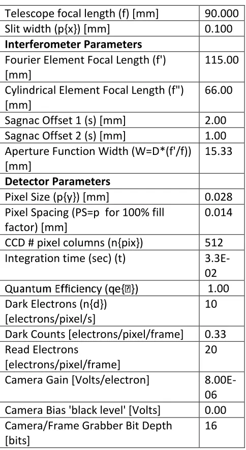
HIMP was used to simulate a 512-element CCD using transmitted source illumination (LOWTRAN) for a US 1976 Standard Atmosphere. The band pass was chosen to lay between 330nm and 1100nm. The major fore-optics, interferometer and detector parameters are in Table 1.

Table 1: HIMP parameters

Telescope focal length (f) [mm] 90.000

Slit width (p{x}) [mm] 0.100

Interferometer Parameters Fourier Element Focal Length (f')

[mm]

115.00

Cylindrical Element Focal Length (f") [mm]

66.00

Sagnac Offset 1 (s) [mm] 2.00 Sagnac Offset 2 (s) [mm] 1.00 Aperture Function Width (W=D*(f'/f))

[mm]

15.33

Detector Parameters

Pixel Size (p{y}) [mm] 0.028

Pixel Spacing (PS=p for 100% fill factor) [mm]

0.014

CCD # pixel columns (n{pix}) 512 Integration time (sec) (t)

3.3E-02 1.00 Dark Electrons (n{d})

[electrons/pixel/s]

10

Dark Counts [electrons/pixel/frame] 0.33 Read Electrons

[electrons/pixel/frame]

20

Camera Gain [Volts/electron] 8.00E-06 Camera Bias 'black level' [Volts] 0.00 Camera/Frame Grabber Bit Depth

[bits]

16

Figure 1. White light interferogram I(x) computed by HIMP. Note the low frequency variation due to the illumination pattern of the CCD by the optics. The centerburst was deliberately placed off center. The x-axis has units of pixels and the y-x-axis on this figure and others has units of total electrons plus noise adjusted for camera gain.

The interferogram I(x) created by HIMP is shown in Figure 1 follows from equation (7), where S(k) is the spectral radiance, I(k) the instrument response function, E(k) the instrument and interferometer

efficiency, V(k) the fringe visibility, s the optical path offset, and k wavenumber. The summation is adjustable within HIMP, typically in 20 wavenumber steps, over the spectral range of choice.

I(x) = ∑S(k)*E(k)*I(k)*(1+V(k)cos (2πks)) (7)

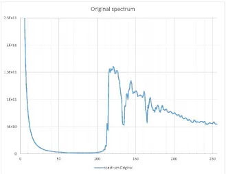
Figure 2. HIMP output spectrum from Figure 1 using FT and IMABS functions in Excel. Note the power distribution at low frenquncies.

Results for L=3 are shown in Figure 3, where the first component has an obvious physical meaning associated with the sensor illumination function of the optics, and where the second and third components correspond to the remainder of the original input signal and various sources of noise.

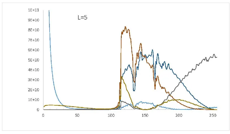
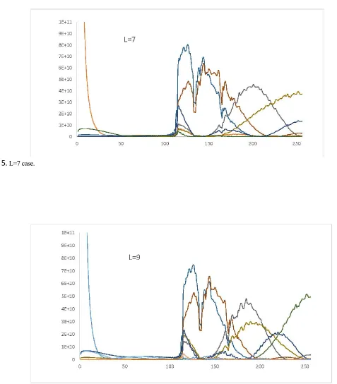
We then explored L=5, L=7 and L=9 cases to see if the increased number of SSA components would suggest association with the various sources of noise and/or sensor attributes introduced by the simulation (e.g., read noise dark noise, top hat sampling--band pass independent, and photon noise--band pass dependent).

The individual components for L=5, 7, 9 cases are shown in the Figures below which are coplotted with a common scale.

Figure 3. L=3 case. The 1st component is associated with the illumination function of the optics (low frequency), the 2nd and 3rd components with the input signal and various sources of noise.

Figure 4. L=5 case. The 1st component (light blue, leftmost) is associated with the optics illumination function. The 2nd and 3rd components (red and dark blue) contain information from the Lowtran input to HIMP.

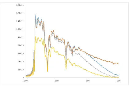
Figure 5. L=7 case.

Figure 6. L=9 case. Sucessive peaks correspond to higher frequency components.

The general pattern for L= (3, 5, 7, 9) is that SSA reproduces the original HIMP signal with the components of each series L, with successive components corresponding to regimes of higher frequency, although for small values of L various spectral features are accommodated by multiple components. In all cases, the low frequency variation contained in the HIMP output that was introduced by the optics illumination function is recovered by the 1st component. The remaining components then account for the remainder of the HIMP (signal+noise) as shown in Figure 2.

To explore how to utilize SSA to remove sources of system or sensor noise, we compared several systematic combination of components for each L to the original spectral distribution used by HIMP to generate the output interferogram (and spectra).

Figure 7. Lowtran input provided to HIMP.

Figure 8. Use of SSA to recover the input spectrum shown in Fig 7 for various values of L with L=3 at the bottom and L=9 at the top, plotted with excluded components (e.g., L=5 (1, 4) is plotted using only the 2nd, 3rd and 4th component of L=5).

SSA provides a physics-based analytical framework for FT interferogram hyperspectral image data that utilizes an adaptive basis, allowing removal of low frequency variations introduced by its optical system and sensor as well as high frequency variations that lay outside the band pass of the detector. SSA extracts a variety of sources of noise or patterns where each of the L-components are associated with specific frequency-specific sources or physical process. We plan future work into using SSA to analyze 2-D hyperspectral data (the second dimension being the single spatial dimension found on each image frame), further investigation of how noise distribution among various components for different values of L, and how the top hat function influences the recovery of both spatial and spectral information.

Acknowledgment. We thank Strathclyde University for hosting JBR during research leave in spring of 2015.

1. J. B. Rafert, Hyperspectral Imaging and Applications Conference, Coventry, U.K., (2014). 2. N. Golyandina, and A. Zhigljavsky, Singular Spectrum Analysis for Time Series, Springer, (2013). 3. N. Golyandina, V. Nekrutkin, and A. A. Zhigljavsky. Chapman-Hall/CRC, 2001.

4. D. S. Broomhead and G. P. King, Physica D, vol. 20, no. 2, (1986).

5. D. S. Broomhead and G. P. King, in Sarkar S (ed) Nonlinear Phenomena and Chaos. Adam Hilger, (Bristol, 1986).

6. N. Golyandina and D. Stepanov. in Proc. of the 5th St. Petersburg Workshop on Simulation, vol. 293, (2005). 7. N. Golyandina and K. D. Usevich, in Matrix Methods: Theory, Algorithms, Applications, (2010).

8. L. J. Rodríguez-Aragón and A. Zhigljavsky, Statistics and Its Interface, vol. 3, (2010).

9. J. Zabalza, J. Ren, Z. Wang, S. Marshall, and J. Wang, IEEE Geoscience and Remote Sensing Letters, 11(11), (2014).

10.J. Zabalza, J. Ren, J. Han, H. Zhao, S. Li, and S. Marshall, IEEE Transactions on Geoscience and Remote Sensing, (2015).

11.J. Zabalza, J. Ren, Z. Wang, H. Zhao, J. Wang, and S. Marshall, IEEE Journal of Selected Topics in Earth

Observation and Remote Sensing, (2014).

12.Bruce Rafert, R. Glenn Seller, Leonard J. Otten III, Proc. SPIE 2480, Imaging Spectroscopy, 410 (1995). 13.Andrew D. Meigs, Eugene W. Butler, Bernard A. Jones, Leonard John Otten III, R. Glenn Sellar, Bruce Rafert,

Proc. SPIE 2819, Imaging Spectrometry II, 278 (1996).

14.J. Bruce Rafert, Leonard J. Otten, Eugene W. Butler, Andrew D. Meigs, Laser Focus World, (2001).

Fig. 1. Figure 1. White light interferogram I(x) computed by HIMP. Note the low frequency variation due to the

illumination pattern of the CCD by the optics. The centerburst was deliberately placed off center. The x-axis has units of pixels and the y-axis on this figure and others has units of total electrons plus noise adjusted for camera gain.

Fig. 3. L=3 case. The 1st component is associated with the illumination function of the optics (low frequency), the

2nd and 3rd components with the input signal and various sources of noise.

Fig. 4. L=5 case. The 1st component (light blue, leftmost) is associated with the optics illumination

Fig. 5. L=7 case.

Fig. 7. Lowtran input provided to HIMP.