Multi-Domain Spectral Methods for Data Reduction in Numerical Relativity Simulations

Reduction in Numerical Relativity Simulations

Brian A. Caimano

[email protected]

Follow this and additional works at:http://scholarworks.rit.edu/theses

Recommended Citation

Multi-Domain Spectral Methods for Data

Reduction in Numerical Relativity

Simulations

by

Brian A Caimano

A Thesis Submitted in Partial Fulfillment of the Requirements for the Degree of Master of Science in Applied and Computational Mathematics

College of Science

School of Mathematical Sciences

Center for Computational Relativity and Gravitation

Rochester Institute of Technology Rochester, NY

Committee Approval:

Matthew J. Hoffman, Ph.D. Date

School of Mathematical Sciences Director of Graduate Programs, SMS

Joshua A. Faber, Ph.D. Date

School of Mathematical Sciences Thesis Advisor

Yosef Zlochower, Ph.D. Date

School of Mathematical Sciences Committee Member

Anthony A. Harkin, Ph.D. Date

Abstract

Contents

1 Introduction 1

2 Multi-Domain Grids 4

2.1 Inner Domain . . . 4

2.2 Intermediate Domains . . . 5

2.3 Infinite Domain . . . 6

3 Data Approximation 8

3.1 Cubic Interpolation . . . 8 3.2 Linear Interpolation . . . 10 3.3 Extrapolation . . . 10

4 Field Splitting 13

5 Multi-Domain Spectral Method 16

5.1 φ Expansion . . . 16 5.2 θ Expansion . . . 17 5.3 ξ Expansion . . . 18

6 Numerical Error 20

6.1 Single-Domain Error . . . 21

6.1.1 Interpolation Error . . . 21 6.1.2 Reconstruction Error . . . 23

6.1.3 Reconstruction Error of an Interpolated Data Set . . . 24

6.2 Two-Domain Error . . . 27

7 Results 29

List of Figures

2.1 Example of multi-domain grids. . . 7

3.1 Depiction of three-dimensional linear interpolation [12]. . . 10

4.1 Heat maps of three candidate splitting functions used for a

singularity located at (−10,0,0) with its binary partner located at (10,0,0) in _R3. . . 15

5.1 Examples of Chebyshev polynomials. . . 19

6.1 The interpolation error, εI, of a linear interpolating routine

as a function of grid spacing, h, over the interval [−10,10] on all axes. The multi-domain grid interpolated onto consists of three domains: an inner domain, an intermediate domain, and a compactified external domain that extends to spacial infinity. 22 6.2 The interpolation error, εI, of a cubic interpolating routine

as a function of grid spacing, h, over the interval [−10,10] on all axes. The multi-domain grid interpolated onto consists of three domains: an inner domain, an intermediate domain, and a compactified external domain that extends to spacial infinity. 23

6.3 The reconstruction error, εR, of the spectral expansion over

6.4 The total error, ε, introduced during the interpolation and subsequent spectral expansion as a function of grid-point spac-ing, h, over the interval [−10,10] in _R3_{. The multi-domain}

grid interpolated onto and then spectrally expanded consists of three domains: an inner domain, one intermediate domain, and a compactified external domain that extends to spacial infinity. The first data series (+) shows the error associated with a multi-domain grid consisting of 1,638 collocation points.

The second data series (×) shows the error associated with

a multi-domain grid consisting of 37,962 collocation points.

The third data series (∗) shows the error associated with a

multi-domain grid consisting of 170,190 collocation points.

The fourth data series () shows the error associated with a

multi-domain grid consisting of 460,530 collocation points.The upper plot utilized a linear interpolation routine and the lower plot utilized a cubic interpolation routine. . . 26

6.5 The total error, ε, introduced during the interpolation and

subsequent spectral expansion as a function of the number of collocation points, N, over the interval [−10,10] in _R3_.

The multi-domain grid interpolated onto and then spectrally expanded consists of three domains: an inner domain, one intermediate domain, and a compactified external domain that extends to spacial infinity. The first data series (+) shows the error associated with a Cartesian grid spacing h = 0.645161. The second data series (×) shows the error associated with a

Cartesian grid spacing h= 0.0660066. The third data series

(∗) shows the error associated with a Cartesian grid spacing

6.6 Results of testing to compare the candidate metric splitting functions effect on accuracy of the spectral expansion of a binary black hole system. The total error, ε, of the interpo-lation and subsequent reconstruction of the original field as

a function of the number of collocation points, N, over the

interval [−128,128] in_R3_{. Each multi-domain grid interpolated}

onto and then spectrally expanded consists of five domains: an inner domain, three intermediate domains, and a compactified external domain that extends to spacial infinity. A data set is plotted for each splitting function given by Equation (4.1) for

n∈ {1,2,4}. . . 28

7.1 Histogram of compressed file sizes (MB) for the three splitting functions tested as a function of the number of collocation points, N, in each multi-domain grid. Each set of collocation points is associated with Equation (4.1) where the left column is calculated with n = 1, the center column is calculated with

List of Tables

7.1 Summary of data compression achieved through multi-domain

spectral methods. The initial grid size consists of 201 points over the interval [−128,128] in _R3_{. . . . . 32}

Chapter 1

Introduction

We have recently passed the century mark for Einstein’s publication of his general theory of relativity [7]. This theory has provided us with the framework to model gravity on scales ranging from terrestrial to cosmological. To date, the general relativistic gravitational model has passed numerous test across multiple length scales. This theory has allowed modeling of large-scale cosmological structures, astrophysical objects such as black holes, neutron stars and other compact bodies, as well as more everyday applications such as GPS systems. Further evidence of the experimental accuracy of general relativity occurred in September 2015, a century after the fundamental predictions of Einstein and Schwarzschild, when the first direct detection of gravitational waves occured. This was the first direct observation of a binary black hole system merging to form a single black hole, in accordance with the predictions of general relativity for the nonlinear dynamics of highly disturbed black holes [1].

Numerical methods to find solutions for valid initial data in general relativity seek the solution of the Hamiltonian constraint [9]

∆ψ+ 1

8K

ab_K

abψ−7 = 0, (1.1)

with boundary conditions ψ → 1 and r → ∞ where the physical extrinsic

curvature, ˆKab_{, is scaled by a conformal factor, ψ, to produce the conformal}

extrinsic curvature, Kab, such that

Kab =ψ2Kˆab. (1.2)

A solution known to work for black hole spacetime configurations, the

Bowen-York solution to the momentum constraints, Kab, for two black holes, with

momentums P1 and P2, and spins S1 and S2, is given by

Kab =

2

X

k=1

3 2r2

k

P_kanb_k+P_kbna_k−(γab−na_knb_k)(Pknk)

+ 3

r3

k

(Sk×nk)anbk+ (Sk×nk)bnak

,

(1.3)

where

rk =

p

(x±b)2_+y2_+z2 _(1.4)

is the coordinate distance to black holes k ∈ {1,2} located at the points (±b,0,0), nk is the radial unit normal vector given by

nk= xa rk

(1.5)

and γ is the conformal three-metric.

refinement using a sequence of nested, logically rectangular meshes on which the partial differential equation is discretized [4]. This technique allows for the adaptation of precision for areas of the model that exhibit dynamic

and/or multi-scale behavior. For our work on initial data, we use Carpet,

an adaptive mesh refinement and multi-patch driver [14], via code found at

http://einsteintoolkit.org/ [10]. These types of problems have extreme data storage requirements since each level of refinement is often quite large, potentially including millions of grid cells, with up to 15 levels of refinement being called upon for the highest resolution simulations [11]. To combat this we look for methods to store data more efficiently, preserving the vast majority of the information content from a simulation while reducing the overall storage requirements.

Chapter 2

Multi-Domain Grids

Using the LORENE numerical libraries [8], we construct a multi-domain grid as described in [5], consisting of an inner spherical domain, intermediate annular domains, and an exterior domain extending to spatial infinity. We divide _R3

into N domains (Dl)0≤l≤N −1 whereN ≥2. Let us denote bySl the boundary

surface between the domains Dl and Dl+1. D0 is simply connected and its

boundary isS0; we call it the nucleus. For 1≤l ≤ N −2, the inner boundary

of Dl is Sl−1 and outer boundary Sl. The infinite domain, DN −1, has inner

boundary SN −2 and extends to spatial infinity [5]. See Figure 2.1 on page 7

for an example.

2.1

Inner Domain

We begin by constructing the mapping

[0,1]×[0, π]×[0,2π)→ D0, (ξ, θ0, φ0)7→(r, θ, φ), (2.1)

where ξ= 0 corresponds to the origin [5]. We take the form of mapping 2.1

to be

r =R0(ξ, θ0, φ0), (2.2)

θ =θ0, (2.3)

φ =φ0, (2.4)

whereR0(ξ, θ, φ) satisfies

R0(1, θ, φ) =S0(θ, φ) (2.5)

since the domain boundaries coincide with ξ= 1 [5]. So R0 is defined as

R0(ξ, θ, φ) =α0[ξ+A0(ξ)F0(θ, φ) +B0(ξ)G0(θ, φ)], (2.6)

where

A0(ξ) = 3ξ4−2ξ6, (2.7)

B0(ξ) = (5ξ3−3ξ5)/2, (2.8)

A0 being an even polynomial and B0 being an odd polynomial[5] and

α0 =S0(θ, φ). (2.9)

The functionsF0(θ, φ) andG0(θ, φ) allow the inner domain to be spheroidal

in geometry since it allows for variation in the radial functions A0(ξ) and

B0(ξ) with respect to the angular variables. We are using spherical mappings

so we take F0(θ, φ) =G0(θ, φ) = 0.

2.2

Intermediate Domains

Domains Dl, such that 1 ≤ l ≤ N −2, are intermediate domains and are

constructed with the mapping

[−1,1]×[0, π]×[0,2π)→ Dl, (ξ, θ0, φ0)7→(r, θ, φ) (2.10)

such that the form of mapping 2.10 is

r=Rl(ξ, θ0, φ0), (2.11)

θ =θ0, (2.12)

φ=φ0, (2.13)

whereRl(ξ, θ, φ) satisfies

Rl(−1, θ, φ) =Sl−1(θ, φ), (2.14)

Rl(1, θ, φ) =Sl(θ, φ), (2.15)

so that the inner (outer) boundary of Dl is defined by ξ =−1 (ξ = 1) [5]. Rl

is defined as

where

Al(ξ) = (ξ3−3ξ+ 2)/4, (2.17)

Bl(ξ) = (−ξ3+ 3ξ+ 2)/4 (2.18)

and

αl=

Sl+1(θ, φ)−Sl(θ, φ)

2 , (2.19)

βl=

Sl+1(θ, φ) +Sl(θ, φ)

2 (2.20)

are defined fromSl+1andSl[5]. As with the inner domain, we takeF0(θ, φ) =

G0(θ, φ) = 0.

2.3

Infinite Domain

The external domain, Dext ≡ DN −1, is the outermost domain with inner

boundary Sext ≡ SN −2, which extends to infinity and has the following

mapping:

[−1,1]×[0, π]×[0,2π)→ Dext, (ξ, θ0, φ0)7→(r, θ, φ) (2.21)

such that the form of mapping 2.21 is

r= 1

U(ξ, θ0_{, φ}0₎, (2.22)

θ=θ0, (2.23)

φ=φ0, (2.24)

where

U(ξ, θ, φ) =αext[ξ+Aext(ξ)Fext(θ, φ)−1] (2.25)

is a smooth function that satisfies

U(−1, θ, φ) =Sext(θ, φ)−1, (2.26)

Figure 2.1: Example of multi-domain grids.

and Aext(ξ)≡Al(ξ), as given in section 2.2 [5]. αext and Fext are

αext =

Sext(θ, φ)−1

−2 +Fext(θ, φ)

, (2.28)

Fext(θ, φ)≤0. (2.29)

Chapter 3

Data Approximation

We approximate metric data from a finite Cartesian grid generated by the

Cactus routines within theEinsteinToolkitto the newly constructed multi-domain grid. We utilize trilinear and tricubic approximation routines and then compare the resultant error data to expected error trends.

3.1

Cubic Interpolation

We first define the distance from the target coordinate, (x, y, z), to the next smaller coordinate with known data, (x0, y0, z0), along each axis, so we have

xd=

(x−x0)

(x1−x0)

, (3.1)

yd=

(y−y0)

(y1−y0)

, (3.2)

zd=

(z−z0)

(z1 −z0)

. (3.3)

Let V[xi, yj, zk] be the function value at (xi, yj, zk) for i, j, k∈[−1,2].

Inter-polating first along the x-axis, we have

cjk =V(x−1, yj, zk)

xd(xd−1)(xd−2) −6

+V(x0, yj, zk)

(xd+ 1)(xd−1)(xd−2)

2

+V(x1, yj, zk)

(xd+ 1)xd(xd−2) −2

+V(x2, yj, zk)

(xd+ 1)xd(xd−1)

6 ,

(3.4)

wherej, k ∈[−1,2]. Next we interpolate along the y-axis

ci =c−1,i

yd(yd−1)(yd−2) −6

+c0,i

(yd+ 1)(yd−1)(yd−2)

2

+c1,i

(yd+ 1)yd(yd−2) −2

+c2,i

(yd+ 1)yd(yd−1)

6 ,

(3.5)

for i∈[−1,2]. We then interpolate along the z-axis

c=c−1

zd(zd−1)(zd−2) −6

+c0

(zd+ 1)(zd−1)(zd−2)

2

+c1

(zd+ 1)zd(zd−2) −2

+c2

(zd+ 1)zd(zd−1)

6 ,

(3.6)

3.2

Linear Interpolation

We again define the distance from the target coordinate, (x, y, z), to the next smaller coordinate with known data, (x0, y0, z0), along each axis, so we have

xd=

(x−x0)

(x1−x0)

, (3.7)

yd=

(y−y0)

(y1−y0)

, (3.8)

zd=

(z−z0)

(z1 −z0)

. (3.9)

Let V[xi, yj, zk] be the function value at (xi, yj, zk) for i, j, k ∈[0,1].

Interpo-lating first along the x-axis, we have

cjk =V[x0, yj, zk](1−xd) +V[x1, yj, zk]xd, (3.10)

wherej, k ∈[0,1]. Next we interpolate along the y-axis,

ci =c0,i(1−yd) +c1,iyd. (3.11)

We then interpolate along the z-axis,

c=c0(1−zd) +c1zd, (3.12)

wherec is the approximate function value at the target coordinate.

Figure 3.1: Depiction of three-dimensional linear interpolation [12].

3.3

Extrapolation

coordinate origin, well beyond the extent of the rectangular grid used by the EinsteinToolkit, to perform the original numerical simulation. Thus, we require a method to take data from the finite-volume Cartesian grid and extrapolate it to arbitrary distances. In doing so, we can take advantage of the fact that all general relativistic field quantities under consideration have known power law fall-off behavior proprtional with distance. Below, we describe our method for fields that exhibit a 1/r fall-off behavior, with obvious generalizations for other power law indices.

For target coordinates falling outside the rectangular grid of original numerical simulation data, V, which we assume is centered at the origin, we calculate the ratios

xratio=

x ∂Vx , (3.13)

yratio =

y ∂vy , (3.14)

zratio =

z ∂Vz , (3.15)

where∂V is the boundary of V and∂Vx,∂Vx, and ∂Vx are the boundaries of V in each axis.

We map a new set of target coordinates, (x0, y0, z0), onto ∂V along the line segment connecting the points (0,0,0) and (x0, y0, z0) defined by

x=x0ζ, (3.16)

y=y0ζ, (3.17)

z =z0ζ, (3.18)

whereζ ∈[0,1].

Solving the line equations for the point (x0, y0, z0) we letζ = _α1, so we have

x0 = x0

α, (3.19)

y0 = y0

α, (3.20)

z0 = z0

α, (3.21)

We interpolate the new target coordinate, (x0, y0, z0), in the same manner as given in Section 3.2. We then scale the resultant approximation, c0, to obtain the approximated function value at the original target coordinate

c= c 0

α, (3.22)

wherec is the approximate function value at the target coordinate. This scaling gives us the desired metric behaviour

lim

Chapter 4

Field Splitting

It is possible to generate a valid spacetime solution for multiple black holes using superposition for their respective extrinsic curvatures, given the linear nature of the momentum constraint. One may then solve for the conformal factor numerically. Given this breakdown, it is natural to view every field quantity, including the metric components, as representing superpositions of terms taking their source as each of the two black holes, respectively. In

this picture, we can decompose every metric quantity into the form F =

fbkgrd+f1+f2, where fbkgrd describes the asymptotic behavior of the field,

and f1 and f2 describe the local structure of spacetime around each black

hole. Splitting the black hole metrics into two spherical domains allows us to utilize spectral methods on the system when reconstruction of the metrics is desired, but this requires us to choose how we will determine the respective

values of f1 and f2 at a given point. To achieve this, we have to pick an

appropriate function, which we call the splitting function, to scale the metric values at each collocation point such that it that minimizes the error of the reconstructed metrics. The function has to account for the mass of, and distance from, each sigularity, thus adjusting the weight given to each point on the multi-domain grids.

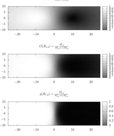
The splitting function candidates we investigate are

g(Ri,j) =

(Mi,jRi,j)n

(Mi,jRi,j) n

+_Mi,jRi,j1

n (4.1)

mi and mj is

Mi,j = mi mj

(4.2)

and the ratio of distances from the point in the multi-domain grid to each singularity is

Ri,j = rj ri

. (4.3)

The candidate function must have some particular properties to establish an accurate metric split. First, to ensure each singularity contributes one-hundred percent of the system’s metric at its origin, F =fi withfj = 0 for i6=j, we have

g(R)→1 as R → ∞ (4.4)

and

g(R)→0 as R →0. (4.5)

This means that we will limit our binary pairs to singularities where g(0) = 1 for both singularities. Second, since we are using an infinte compactified external domain in order to represent all of space, we must have that

g(R)→ 1

2 as R→1 (4.6)

in order to achieve an equal split at the limits of the domain.

This leaves us with the following local values of the metric components:

f1 =g(R1,2)·(F −fbkgrd) (4.7)

and

f2 =g(R2,1)·(F −fbkgrd) (4.8)

G(R1,2) =

R1,2

R1,2+1/R1,2

G(R1,2) =

R21,2

R2

1,2+1/R21,2

g(R1,2) =

R41,2

R4

1,2+1/R14,2

−20 −10 0 10 20

−10 −5 0 5 10 0 0.1 0.2 0.3 0.4 0.5 0.6 0.7 0.8 0.9 1

−20 −10 0 10 20

−10 −5 0 5 10 0 0.1 0.2 0.3 0.4 0.5 0.6 0.7 0.8 0.9 1

−20 −10 0 10 20

−10 −5 0 5 10 0 0.2 0.4 0.6 0.8 1

Chapter 5

Multi-Domain Spectral Method

The goal of utilizing a multi-domain spectral scheme is to expand each domain as a finite sum. Any singular function can be represented in terms of a Taylor series by

f(x, y, z) = X

i,j,k

ci,j,kxiyjzk. (5.1)

By the usual coordinate transformation we have

f(r, θ, φ) =

M

X

m=−M L

X

`=|m|

r`T(r2) sin|m|θP`−|m|(cosθ)eimφ, (5.2)

whereL and M are positive integers, L > M, P`−|m| is some polynomial of degree `− |m|and T(r2_{) is some even polynomial.}

The spectral expansion will be with repect to (ξ, θ, φ) instead of the

physical coordinates (r, θ, φ). The basis functions are chosen such that they may be put in the form X(ξ)Θ(θ)Φ(φ).

5.1

φ

Expansion

Since φ is periodic, the Fourier series is chosen as the basis functions

Φk(φ) =eikφ,

−Nφ

2 ≤k≤

Nφ

2 , (5.3)

whereNφ is the number of degrees of freedom inφ [5]. The collocation points

are defined as

φk =

2πk Nφ

, k = 0, . . . , Nφ−1 (5.4)

and are equally spaced in [0,2π)[6]. So we have the approximation formula

for the φ expansion

INφfφ(φ) = Nφ/2

X

k=−Nφ/2

akΦk(φ), (5.5)

where

ak =

1

Nφ Nφ−1

X

k=0

fφ(φk)e−ikφk (5.6)

are the discrete Fourier coefficients [6].

5.2

θ

Expansion

In θ we take the basis functions as

Θkj(θ) =

(

cos(jθ), 0≤j ≤Nθ −1 for m even

sin(jθ), 0≤j ≤Nθ −1 for m odd

, (5.7)

whereNθ is the number of degrees of freedom in θ [5]. The collocation points

are defined as

θj = πj Nθ−1

, j = 0, . . . , Nθ−1 (5.8)

and are equally spaced in [0, π] [6]. So we have the approximation formula for the θ expansion

INθfθ(θ) = Nθ−1

X

j=0

ajΘj(θ), (5.9)

where

a0 =

1

Nθ

fθ(θ0) (5.10)

and

aj =

2

Nθ Nθ−1

X

j=1

fθ(θj)e−ijθj (5.11)

5.3

ξ

Expansion

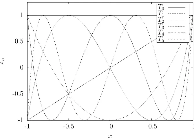
For the nucleus of the multi-domain grids we use the basis functions

Xkji =

(

T2i(ξ), 0≤i≤Nr−1 for j even T2i+1(ξ), 0≤i≤Nr−2 for j odd

, (5.12)

where Nr is the number of degrees of freedom in r, and Tn is the nth degree

Chebyshev polynomial [5]. The collocation points are defined as

ξi = sin

π

2

i Nr−1

, i= 0, . . . , Nr−1 (5.13)

and are spaced to minimize the Runge phenomenon [6]. For the intermediate and external domains we use

Xkji =Ti(ξ) (5.14)

as basis functions, and the collocation points

ξi =−cos

πi Nr−1

, i= 0, . . . , Nr−1. (5.15)

This leaves us with the radial approximation formula

INrfr(ξ) = Nr−1

X

i=0

aiXkji(ξ), (5.16)

where

a0 =

1

Nr

fr(ξ0)T0(ξ0) (5.17)

and

ai =

2

Nr Nr−1

X

i=1

fr(ξi)Ti(ξi) (5.18)

-1 -0.5 0 0.5 1

-1 -0.5 0 0.5 1

Tn

x

T0

T1

T2

T3

T4

T5

Chapter 6

Numerical Error

Error is introduced in two places using this method. The first is when data is interpolated onto the LORENE grids via cubic and linear interpolating routines, and the second is when the field is reconstructed using spectral expansions. The reconstruction error consists of error from the difference between the exact function and the interpolant, as well as truncation error caused by cutting off higher order modes of the series expansion. We look at the error introduced and verify that it follows expected fall-offs based on grid size and interpolation technique.

We compare the error introduced when data is approximated at the collocation points over multiple Cartesian grid sizes. The error calculated is the root-mean-square deviation (RMSD) and represents the difference between approximated values and exact values.

RM SD =

r Pn

k=1(ˆx−x)2

n , (6.1)

where ˆx is the approximated value, xis the exact value, and n is the sample size.

To test the error introduced, we use the function

f(r, θ, φ) =

r2

√

1 +r6

cos(θ) sin(θ)[sin(φ) + cos(φ)] (6.2)

which is exactly representable by the spectral expansion methods used.

6.1

Single-Domain Error

We begin by generating Cartesian grids of varying densities to investigate the expected interpolation error introduced as data is transferred from the Carte-sian grid to the multi-domain grids generated from the LORENE routines. Next, we feed the exact values of Equation (6.2) into the collocation points of the multi-domain grid and compare it to the spectral expansion generated by the LORENE routines at the same points, looking for minimal error, which signifies that the expansion routines work as designed. Finally, we combine both interpolation and spectral expansion and look at the error produced when a Cartesian grid of data generated from Equation (6.2) is interpolated onto a multi-domain grid, spectrally expanded, and then calculated at the original Cartesian grid points to determine the error of a fully reconstructed field. In all cases, the RMSD is then calculated in the standard way using Equation (6.1).

6.1.1

Interpolation Error

Interpolating data onto the LORENE grid will introduce error. We aim to quantify how much is introduced using different Cartesian grid densities. We utilize two interpolation routines: linear and cubic. We expect the linear routine to produce error fall-off approximately ∝h2, and the cubic routine to produce error fall-off approximately ∝h4_.

Figures 6.1 and 6.2 show the interpolation error, εI, as a function of

Cartesian grid point spacing, h, associated with linear and cubic interpolation routines, respectively. We see that the error approximately follows a power

law convergence εI ∝ h−β, as seen by the tracking curve plotted in each

figure, as expected. The Cartesian grids are in the interval [−10,10] and have a varying grid spacing of h= 2.22222 to h= 2×10−8_{. Note that only}

the points in each grid needed for the interpolation are loaded into memory, thus reducing the computational overhead. The multi-domain grid extends to spacial infinity due to the exterior domain compactification. The x-axis is the rectangular grid spacing h, and they-axis is the interpolation error εI. Both

routine may be compared properly over the same domain. From the graph we can see both the linear and cubic interpolation routines exhibit power law fall-off, as expected. We see that saturation begins to occur at approximately

h= 1×10−8 _{in the linear case and occurs at approximately h= 1×10}−4 _in

the cubic case.

10−16 10−14

10−12

10−10

10−8

10−6 10−4 10−2

100

10−8

10−7

10−6

10−5

10−4

10−3

10−2

10−1

100

101

In

terp

olation

Error,

εI

Grid Spacing, h

h2

Figure 6.1: The interpolation error, εI, of a linear interpolating routine as

10−16 10−14

10−12

10−10

10−8

10−6 10−4 10−2

100

10−8

10−7

10−6

10−5

10−4

10−3

10−2

10−1

100

101

Reconstruction

Error,

εR

Grid Spacing, h

h4

Figure 6.2: The interpolation error, εI, of a cubic interpolating routine as

a function of grid spacing, h, over the interval [−10,10] on all axes. The multi-domain grid interpolated onto consists of three domains: an inner domain, an intermediate domain, and a compactified external domain that extends to spacial infinity.

6.1.2

Reconstruction Error

When reconstructing the field with a spectral expansion, we expect error to be introduced into the data. The error is the result of a difference in the exact function and that function’s interpolant, as well as truncation error caused by cutting off higher order modes of the series expansion. We expect the error will become evanescent when a large number of collocation points is used in the multi-domain grid. We verify an exactly representable function in (r, θ, φ) inputted onto the LORENE spectral expansion routine can be extracted as an approximated function with negligible error introduced, confirming the spectral routines work as expected.

As we can see from the results in Figure 6.3, reconstruction error, εR,

routine is provided an exactly representable function. Saturation occurs at approximately 3.5×105 collocation points. After the saturation point, further refinement of the multi-domain grid will not yield better accuracy and will only add to the computational overhead of the routine.

10−18

10−16 10−14

10−12 10−10

10−8

10−6 10−4

103 ₁₀4 ₁₀5 ₁₀6

Reconstruction

Error,

εR

Number of collocation points, N

Figure 6.3: The reconstruction error, εR, of the spectral expansion over an

exactly representable function, as a function of the number of collocation

points, N, in the multi-domain grid. The multi-domain grid used for the

spectral expansion consists of four domains: an inner domain, two intermediate domains, and a compactified external domain that extends to spacial infinity.

6.1.3

Reconstruction Error of an Interpolated Data

Set

from the LORENE routines and approximate the values of the metric at the coordinates in the Cartesian grids in order to compare the original values to the spectrally expanded values. Due to the high number of points needed to calculate the error, we use a reduced sample set.

10−7 10−6

10−5

10−4 10−3 10−2

10−3

10−2

10−1

100 101 T otal Error, ε

Grid Spacing, h

10−10 10−9

10−8

10−7 10−6

10−5

10−4 10−3

10−3

10−2

10−1

100 101 T otal Error, ε

Grid Spacing, h

Figure 6.4: The total error, ε, introduced during the interpolation and

subsequent spectral expansion as a function of grid-point spacing, h, over

the interval [−10,10] in _R3. The multi-domain grid interpolated onto and then spectrally expanded consists of three domains: an inner domain, one intermediate domain, and a compactified external domain that extends to spacial infinity. The first data series (+) shows the error associated with a

multi-domain grid consisting of 1,638 collocation points. The second data

series (×) shows the error associated with a multi-domain grid consisting of 37,962 collocation points. The third data series (∗) shows the error associated with a multi-domain grid consisting of 170,190 collocation points. The fourth data series () shows the error associated with a multi-domain grid consisting of 460,530 collocation points.The upper plot utilized a linear interpolation routine and the lower plot utilized a cubic interpolation routine.

10−7 10−6

10−5

10−4 10−3 10−2

103 ₁₀4 ₁₀5 ₁₀6

T

otal

Error,

ε

Number of Collocation Points, N

10−10 10−9

10−8

10−7 10−6

10−5

10−4 10−3

103 ₁₀4 ₁₀5 ₁₀6

T

otal

Error,

ε

Number of Collocation Points, N

Figure 6.5: The total error, ε, introduced during the interpolation and

subsequent spectral expansion as a function of the number of collocation points,

N, over the interval [−10,10] in_R3. The multi-domain grid interpolated onto and then spectrally expanded consists of three domains: an inner domain, one intermediate domain, and a compactified external domain that extends to spacial infinity. The first data series (+) shows the error associated with

a Cartesian grid spacing h = 0.645161. The second data series (×) shows

the error associated with a Cartesian grid spacing h= 0.0660066. The third

data series (∗) shows the error associated with a Cartesian grid spacing

h = 0.00666001. The upper plot utilized a linear interpolation routine and the lower plot utilized a cubic interpolation routine.

6.2

Two-Domain Error

error of the spectral expansion.

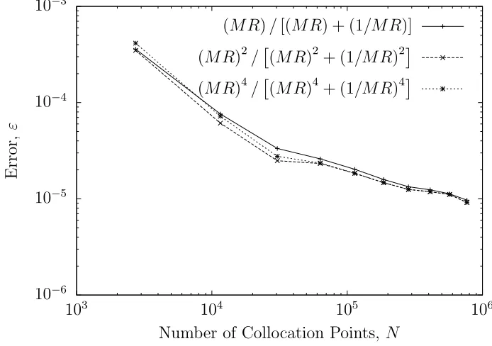
Figure 6.6 shows the total error, ε, from each of the candidate splitting functions, defined in Section 4, as a function of the number of collocation points, N, used in the calculation. The original field was given by Equation

(6.2) over the domain [−128,128] in _R3 with the black holes centered at

(±10,0,0). We see each splitting function resulting in approximately equal error.

10−6

10−5

10−4

10−3

103 ₁₀4 ₁₀5 ₁₀6

Error,

ε

Number of Collocation Points, N

(M R)/[(M R) + (1/M R)]

(M R)2/

(M R)2+ (1/M R)2

(M R)4/

(M R)4+ (1/M R)4

Figure 6.6: Results of testing to compare the candidate metric splitting functions effect on accuracy of the spectral expansion of a binary black hole system. The total error,ε, of the interpolation and subsequent reconstruction of the original field as a function of the number of collocation points, N, over the interval [−128,128] in _R3_{. Each multi-domain grid interpolated onto and}

Chapter 7

Results

Our goal was to minimize the storage requirements of general relativistic evolution simulations and, at the same time, minimize the error introduced by the compression routine. In order to do this we needed to consider both the initial Cartesian grid density used for the interpolation, and the multi-domain grid density used for the spectral expansion.

In terms of the optimal grid density for our interpolation routines, we are looking for a Cartesian grid density that achieves maximum accuracy. For the cubic interpolation routine, this occurs below the grid spacing h= 1×10−4_,

keeping in mind that the outer voxels utilize a linear interpolation routine, and saturation occurs below h = 1×10−8 in this case. If the outer voxels contain relatively smooth data then the saturation density of the cubic routine should suffice, otherwise the linear saturation density should be considered, although the computational overhead will be greater.

To reconstruct the metrics with suitable accuracy, the spectral expansion should utilize grid densities that, like in the case of the optimal interpolation grid densities, minimize error and computational requirements. This occurs at approximately 3.5×105 _{collocation points in our test cases. Some variabililty}

can occur here due to the number of domains used in the reconstruction and the interval of each domain. Optimally, the highest density of collocation points will occur where the data is most dynamic (e.g. in the immediate area of the singularity, near an accretion disk, etc...).

In order to optimize accuracy, we tested multiple functions to decouple the black holes’ metric fields. The different functions assigned differing amounts of the combined metric F to each isolated metric f1 and f2.

equal error. No one function stands out as more accurate, though at higher collocation point counts, greater than approximately 105 points per grid, the three functions error converges to the same value. From a computational perspective, choosing the function

g(Ri,j) =

(Mi,jRi,j)

(Mi,jRi,j) +

1

Mi,jRi,j

(7.1)

will lower the computational overhead required since fewer exponents are used, though the savings would be negligible.

Figure 7.1 shows the relative compressed file sizes for the three splitting functions defined in Section 4 over varying multi-domain grid densities. No appreciable difference in file storage size can be distinguished between different splitting functions, which is to be expected since the storage requirements are a function of total data points, not the value of the data itself.

Now, when comparing the compressed data to the original data in terms of storage space, we have a significant reduction in storage requirements. Table 7.1 summarizes the data compression achieved by our routines. This level of compression allows an immense amount of data storage. A metric field could be stored for future work and, due to the nature of the spectral

expansion, can be reconstructed in any desired configuration. It is not

necessary to reconstruct the original field, as the expansion can accept any arbitrary coordinate (r, θ, φ). In addition, the use of multiple domains allows this method to be utilized in not only black hole calculations, where the field is smooth everywhere but at the singularity, but also in calculations involving objects where the surface is non-differentiable. By aligning the boundary surface, S0, of the nucleus, D0, we avoid the issues associated with

0 2 4 6 8 10 12 14

1638 6930 _{18270 37962 68310}

113850 186030 283650 410550 570570

File

Size,

MB

Number of Collocation Points, N

Figure 7.1: Histogram of compressed file sizes (MB) for the three splitting functions tested as a function of the number of collocation points, N, in each multi-domain grid. Each set of collocation points is associated with Equation

(4.1) where the left column is calculated with n = 1, the center column is

Collocation Points Size (MB) Original Size (MB) % Reduction Error 2730 0.052680

568.6

99.99% 0.000359739 11550 0.235448 99.96% 7.61397e-05 30450 0.638737 99.89% 3.33353e-05 63270 1.345334 99.76% 2.59806e-05 113850 2.447111 99.57% 2.0246e-05 186030 4.023237 99.29% 1.58614e-05 283650 6.163660 98.92% 1.33373e-05 410550 8.959538 98.42% 1.24144e-05 570570 12.491530 97.80% 1.12602e-05 767550 16.847986 97.04% 9.67996e-06

References

T. Chalermsongsak, S. J. Chamberlin, M. Chan, S. Chao, P. Charlton, E. Chassande-Mottin, H. Y. Chen, Y. Chen, C. Cheng, A. Chincarini, A. Chiummo, H. S. Cho, M. Cho, J. H. Chow, N. Christensen, Q. Chu, S. Chua, S. Chung, G. Ciani, F. Clara, J. A. Clark, F. Cleva, E. Coccia, P.-F. Cohadon, A. Colla, C. G. Collette, L. Cominsky, M. Constan-cio, A. Conte, L. Conti, D. Cook, T. R. Corbitt, N. Cornish, A. Corsi, S. Cortese, C. A. Costa, M. W. Coughlin, S. B. Coughlin, J.-P. Coulon, S. T. Countryman, P. Couvares, E. E. Cowan, D. M. Coward, M. J. Cow-art, D. C. Coyne, R. Coyne, K. Craig, J. D. E. Creighton, T. D. Creighton, J. Cripe, S. G. Crowder, A. M. Cruise, A. Cumming, L. Cunningham, E. Cuoco, T. D. Canton, S. L. Danilishin, S. D’Antonio, K. Danzmann, N. S. Darman, C. F. Da Silva Costa, V. Dattilo, I. Dave, H. P. Dav-eloza, M. Davier, G. S. Davies, E. J. Daw, R. Day, S. De, D. DeBra, G. Debreczeni, J. Degallaix, M. De Laurentis, S. Del´eglise, W. Del Pozzo, T. Denker, T. Dent, H. Dereli, V. Dergachev, R. T. DeRosa, R. De Rosa, R. DeSalvo, S. Dhurandhar, M. C. D´ıaz, L. Di Fiore, M. Di Giovanni, A. Di Lieto, S. Di Pace, I. Di Palma, A. Di Virgilio, G. Dojcinoski, V. Dolique, F. Donovan, K. L. Dooley, S. Doravari, R. Douglas, T. P. Downes, M. Drago, R. W. P. Drever, J. C. Driggers, Z. Du, M. Ducrot, S. E. Dwyer, T. B. Edo, M. C. Edwards, A. Effler, H.-B. Eggenstein, P. Ehrens, J. Eichholz, S. S. Eikenberry, W. Engels, R. C. Essick, T. Etzel, M. Evans, T. M. Evans, R. Everett, M. Factourovich, V. Fafone, H. Fair, S. Fairhurst, X. Fan, Q. Fang, S. Farinon, B. Farr, W. M. Farr, M. Favata, M. Fays, H. Fehrmann, M. M. Fejer, D. Feldbaum, I. Ferrante, E. C. Ferreira, F. Ferrini, F. Fidecaro, L. S. Finn, I. Fiori, D. Fiorucci, R. P. Fisher, R. Flaminio, M. Fletcher, H. Fong, J.-D. Fournier, S. Franco, S. Frasca, F. Frasconi, M. Frede, Z. Frei, A. Freise, R. Frey, V. Frey, T. T. Fricke, P. Fritschel, V. V. Frolov, P. Fulda, M. Fyffe, H. A. G. Gabbard, J. R. Gair, L. Gammaitoni, S. G. Gaonkar, F. Garufi, A. Gatto, G. Gaur, N. Gehrels, G. Gemme, B. Gendre, E. Genin, A. Gennai, J. George, L. Gergely, V. Germain, A. Ghosh, A. Ghosh, S. Ghosh, J. A. Giaime, K. D. Giardina, A. Giazotto, K. Gill, A. Glaefke, J. R. Gleason, E. Goetz,

R. Goetz, L. Gondan, G. Gonz´alez, J. M. G. Castro, A. Gopakumar,

Ham-mond, M. Haney, M. M. Hanke, J. Hanks, C. Hanna, M. D. Hannam, J. Hanson, T. Hardwick, J. Harms, G. M. Harry, I. W. Harry, M. J. Hart, M. T. Hartman, C.-J. Haster, K. Haughian, J. Healy, J. Heefner, A. Heidmann, M. C. Heintze, G. Heinzel, H. Heitmann, P. Hello, G. Hem-ming, M. Hendry, I. S. Heng, J. Hennig, A. W. Heptonstall, M. Heurs, S. Hild, D. Hoak, K. A. Hodge, D. Hofman, S. E. Hollitt, K. Holt, D. E. Holz, P. Hopkins, D. J. Hosken, J. Hough, E. A. Houston, E. J. Howell, Y. M. Hu, S. Huang, E. A. Huerta, D. Huet, B. Hughey, S. Husa, S. H. Huttner, T. Huynh-Dinh, A. Idrisy, N. Indik, D. R. Ingram, R. Inta, H. N. Isa, J.-M. Isac, M. Isi, G. Islas, T. Isogai, B. R. Iyer, K. Izumi, M. B. Jacobson, T. Jacqmin, H. Jang, K. Jani, P. Jaranowski, S. Jawahar, F. Jim´enez-Forteza, W. W. Johnson, N. K. Johnson-McDaniel, D. I. Jones, R. Jones, R. J. G. Jonker, L. Ju, K. Haris, C. V. Kalaghatgi, V. Kalogera, S. Kandhasamy, G. Kang, J. B. Kanner, S. Karki, M. Kasprzack, E. Kat-savounidis, W. Katzman, S. Kaufer, T. Kaur, K. Kawabe, F. Kawazoe, F. K´ef´elian, M. S. Kehl, D. Keitel, D. B. Kelley, W. Kells, R. Kennedy, D. G. Keppel, J. S. Key, A. Khalaidovski, F. Y. Khalili, I. Khan, S. Khan, Z. Khan, E. A. Khazanov, N. Kijbunchoo, C. Kim, J. Kim, K. Kim, N.-G. Kim, N. Kim, Y.-M. Kim, E. J. King, P. J. King, D. L. Kinzel, J. S. Kissel, L. Kleybolte, S. Klimenko, S. M. Koehlenbeck, K. Kokeyama, S. Koley, V. Kondrashov, A. Kontos, S. Koranda, M. Korobko, W. Z.

Korth, I. Kowalska, D. B. Kozak, V. Kringel, B. Krishnan, A. Kr´olak,

C. Krueger, G. Kuehn, P. Kumar, R. Kumar, L. Kuo, A. Kutynia, P. Kwee, B. D. Lackey, M. Landry, J. Lange, B. Lantz, P. D. Lasky, A. Lazzarini, C. Lazzaro, P. Leaci, S. Leavey, E. O. Lebigot, C. H. Lee, H. K. Lee, H. M. Lee, K. Lee, A. Lenon, M. Leonardi, J. R. Leong, N. Leroy, N. Letendre, Y. Levin, B. M. Levine, T. G. F. Li, A. Libson, T. B. Littenberg, N. A. Lockerbie, J. Logue, A. L. Lombardi, L. T. London, J. E. Lord, M. Lorenzini, V. Loriette, M. Lormand, G. Lo-surdo, J. D. Lough, C. O. Lousto, G. Lovelace, H. L¨uck, A. P. Lundgren, J. Luo, R. Lynch, Y. Ma, T. MacDonald, B. Machenschalk, M. MacInnis,

D. M. Macleod, F. Maga˜na Sandoval, R. M. Magee, M. Mageswaran,

McClelland, S. McCormick, S. C. McGuire, G. McIntyre, J. McIver, D. J. McManus, S. T. McWilliams, D. Meacher, G. D. Meadors, J. Meidam, A. Melatos, G. Mendell, D. Mendoza-Gandara, R. A. Mercer, E. Merilh, M. Merzougui, S. Meshkov, C. Messenger, C. Messick, P. M. Meyers, F. Mezzani, H. Miao, C. Michel, H. Middleton, E. E. Mikhailov, L. Mi-lano, J. Miller, M. Millhouse, Y. Minenkov, J. Ming, S. Mirshekari, C. Mishra, S. Mitra, V. P. Mitrofanov, G. Mitselmakher, R. Mittleman, A. Moggi, M. Mohan, S. R. P. Mohapatra, M. Montani, B. C. Moore, C. J. Moore, D. Moraru, G. Moreno, S. R. Morriss, K. Mossavi, B. Mours, C. M. Mow-Lowry, C. L. Mueller, G. Mueller, A. W. Muir, A. Mukherjee, D. Mukherjee, S. Mukherjee, N. Mukund, A. Mullavey, J. Munch, D. J. Murphy, P. G. Murray, A. Mytidis, I. Nardecchia, L. Naticchioni, R. K. Nayak, V. Necula, K. Nedkova, G. Nelemans, M. Neri, A. Neunzert, G. Newton, T. T. Nguyen, A. B. Nielsen, S. Nissanke, A. Nitz, F. Nocera, D. Nolting, M. E. N. Normandin, L. K. Nuttall, J. Oberling, E. Ochsner, J. O’Dell, E. Oelker, G. H. Ogin, J. J. Oh, S. H. Oh, F. Ohme, M. Oliver, P. Oppermann, R. J. Oram, B. O’Reilly, R. O’Shaughnessy, C. D. Ott, D. J. Ottaway, R. S. Ottens, H. Overmier, B. J. Owen, A. Pai, S. A. Pai, J. R. Palamos, O. Palashov, C. Palomba, A. Pal-Singh, H. Pan, Y. Pan, C. Pankow, F. Pannarale, B. C. Pant, F. Paoletti, A. Paoli, M. A. Papa, H. R. Paris, W. Parker, D. Pascucci, A. Pasqualetti, R. Passaquieti, D. Passuello, B. Patricelli, Z. Patrick, B. L. Pearlstone, M. Pedraza, R. Pedurand, L. Pekowsky, A. Pele, S. Penn, A. Perreca, H. P. Pfeif-fer, M. Phelps, O. Piccinni, M. Pichot, M. Pickenpack, F. Piergiovanni, V. Pierro, G. Pillant, L. Pinard, I. M. Pinto, M. Pitkin, J. H. Poeld, R. Poggiani, P. Popolizio, A. Post, J. Powell, J. Prasad, V. Predoi, S. S. Premachandra, T. Prestegard, L. R. Price, M. Prijatelj, M. Principe, S. Privitera, R. Prix, G. A. Prodi, L. Prokhorov, O. Puncken, M. Pun-turo, P. Puppo, M. P¨urrer, H. Qi, J. Qin, V. Quetschke, E. A. Quintero, R. Quitzow-James, F. J. Raab, D. S. Rabeling, H. Radkins, P. Raffai, S. Raja, M. Rakhmanov, C. R. Ramet, P. Rapagnani, V. Raymond, M. Razzano, V. Re, J. Read, C. M. Reed, T. Regimbau, L. Rei, S. Reid, D. H. Reitze, H. Rew, S. D. Reyes, F. Ricci, K. Riles, N. A. Robertson, R. Robie, F. Robinet, A. Rocchi, L. Rolland, J. G. Rollins, V. J. Roma,

J. D. Romano, R. Romano, G. Romanov, J. H. Romie, D. Rosi´nska,

S. Rowan, A. R¨udiger, P. Ruggi, K. Ryan, S. Sachdev, T. Sadecki,

Sanders, J. R. Sanders, B. Sassolas, B. S. Sathyaprakash, P. R. Saulson, O. Sauter, R. L. Savage, A. Sawadsky, P. Schale, R. Schilling, J. Schmidt, P. Schmidt, R. Schnabel, R. M. S. Schofield, A. Sch¨onbeck, E. Schreiber, D. Schuette, B. F. Schutz, J. Scott, S. M. Scott, D. Sellers, A. S. Sengupta, D. Sentenac, V. Sequino, A. Sergeev, G. Serna, Y. Setyawati, A. Sevigny, D. A. Shaddock, T. Shaffer, S. Shah, M. S. Shahriar, M. Shaltev, Z. Shao, B. Shapiro, P. Shawhan, A. Sheperd, D. H. Shoemaker, D. M. Shoemaker, K. Siellez, X. Siemens, D. Sigg, A. D. Silva, D. Simakov, A. Singer, L. P. Singer, A. Singh, R. Singh, A. Singhal, A. M. Sintes, B. J. J. Slagmolen, J. R. Smith, M. R. Smith, N. D. Smith, R. J. E. Smith, E. J. Son, B. So-razu, F. Sorrentino, T. Souradeep, A. K. Srivastava, A. Staley, M. Steinke, J. Steinlechner, S. Steinlechner, D. Steinmeyer, B. C. Stephens, S. P. Stevenson, R. Stone, K. A. Strain, N. Straniero, G. Stratta, N. A. Strauss, S. Strigin, R. Sturani, A. L. Stuver, T. Z. Summerscales, L. Sun, P. J. Sutton, B. L. Swinkels, M. J. Szczepa´nczyk, M. Tacca, D. Talukder, D. B.

Tanner, M. T´apai, S. P. Tarabrin, A. Taracchini, R. Taylor, T. Theeg,

M. P. Thirugnanasambandam, E. G. Thomas, M. Thomas, P. Thomas, K. A. Thorne, K. S. Thorne, E. Thrane, S. Tiwari, V. Tiwari, K. V. Tokmakov, C. Tomlinson, M. Tonelli, C. V. Torres, C. I. Torrie, D. T¨oyr¨a, F. Travasso, G. Traylor, D. Trifir`o, M. C. Tringali, L. Trozzo, M. Tse, M. Turconi, D. Tuyenbayev, D. Ugolini, C. S. Unnikrishnan, A. L. Urban, S. A. Usman, H. Vahlbruch, G. Vajente, G. Valdes, M. Vallisneri, N. van Bakel, M. van Beuzekom, J. F. J. van den Brand, C. Van Den Broeck, D. C. Vander-Hyde, L. van der Schaaf, J. V. van Heijningen, A. A. van

Veggel, M. Vardaro, S. Vass, M. Vas´uth, R. Vaulin, A. Vecchio, G.

Ve-dovato, J. Veitch, P. J. Veitch, K. Venkateswara, D. Verkindt, F. Vetrano,

A. Vicer´e, S. Vinciguerra, D. J. Vine, J.-Y. Vinet, S. Vitale, T. Vo,

M. Zanolin, J.-P. Zendri, M. Zevin, F. Zhang, L. Zhang, M. Zhang, Y. Zhang, C. Zhao, M. Zhou, Z. Zhou, X. J. Zhu, M. E. Zucker, S. E. Zuraw, and J. Zweizig. Observation of gravitational waves from a binary black hole merger. Phys. Rev. Lett., 116:061102, Feb 2016.

[2] R. Arnowitt, S. Deser, and C. W. Misner. The dynamics of general

relativity. Gravitation: An Introduction to Current Research, pages

227–265, 1962.

[3] T. W. Baumgarte and S. L. Shapiro. On the numerical integration of Einstein’s field equations. Phys. Rev., D59:024007, 1999.

[4] M. J. Berger and P. Colella. Local adaptive mesh refinement for shock

hydrodynamics. Journal of Computational Physics, 82:64–84, May 1989.

[5] S. Bonazzola, E. Gourgoulhon, and J.-A. Marck. Numerical approach for high precision 3d relativistic star models. Phys. Rev. D, 58:104020, Oct 1998.

[6] C. Canuto, M. Hussaini, A. Quarteroni, and T. Zang. Spectral Methods:

Evolution to Complex Geometries and Application to Fluid Dynamics.

Springer Berlin Heidelburg New York, 2007.

[7] A. Einstein. Die Grundlage der allgemeinen Relativit¨atstheorie. Annalen der Physik, 354:769–822, 1916.

[8] E. Gourgoulhon, P. Grandcl´ement, J.-A. Marck, J. Novak, and

K. Taniguchi. LORENE: Spectral methods differential equations solver. Astrophysics Source Code Library, Aug. 2016.

[9] B. James. Initial Data for a Binary Black Hole System. Unpublished Thesis, 2013.

[10] F. L¨offler, J. Faber, E. Bentivegna, T. Bode, P. Diener, R. Haas, I. Hinder, B. C. Mundim, C. D. Ott, E. Schnetter, G. Allen, M. Campanelli, and P. Laguna. The Einstein Toolkit: A Community Computational

Infrastructure for Relativistic Astrophysics. Class. Quantum Grav.,

29(11):115001, 2012.

[12] Marmelad, 2008. http://creativecommons.org/licenses/by-sa/3.0/deed.en.

[13] S. C. Noble, J. H. Krolik, and J. F. Hawley. Direct calculation of

the radiative efficiency of an accretion disk around a black hole. The

Astrophysical Journal, 692(1):411, 2009.

[14] E. Schnetter, 2011. http://www.carpetcode.org/.

[15] M. Shibata and T. Nakamura. Evolution of three-dimensional

gravita-tional waves: Harmonic slicing case. Phys. Rev. D, 52:5428–5444, Nov