Internet Traffic Modeling and Future Technology
Implications
Moshe Zukerman , Timothy D. Neame
†and Ronald G. Addie
‡,† ARC Special Research Centre for Ultra-Broadband Information Networks (CUBIN), Department of Electrical and Electronic Engineering,
The University of Melbourne, Victoria 3010, Australia Email:
m.zukerman, t.neame @ee.mu.oz.au
Moshe Zukerman is visiting the Department of Electronic Engineering, City University of Hong Kong, between November 2002 and July 2003.
‡Department of Mathematics and Computing, University of Southern Queensland
Email: [email protected]
Abstract— This paper presents the Poisson Pareto burst
pro-cess (PPBP) as a simple but accurate model for Internet traffic. It presents formulae relating the parameters of the PPBP to measurable traffic statistics, and describes a technique for fitting the PPBP to a given traffic stream. The PPBP is shown to accurately predict the queueing performance of a sample trace of aggregated Internet traffic. Using the traffic model, we predict that in few years, efficient statistical multiplexing will lead to efficient optical Internet.
I. INTRODUCTION
For over a quarter of a century researchers have been looking for a stochastic process which could be used as an 1 accurate and simple model for traffic in packet switched networks. The criteria for such a stochastic process are:
(i) It is defined by a small number of parameters.
(ii) If these parameters are fitted using measurable statistics of an actual traffic stream the following will be achieved:
1) the first and second order statistics including the autoco-variance function of the stochastic process (the model) will match those of the actual traffic stream, and 2) if fed through a single server queue (SSQ), performance
results for the model will accurately predict those of the real traffic stream fed into an identical SSQ. This must be true for a wide range of buffer sizes as well as for a wide range of service rates.
(iii) It is amenable to analysis.
If the process also parallels the nature of the traffic that is being modeled, this will give maximum confidence in its usefulness.
In this paper we examine the Poisson Pareto burst process (PPBP) and demonstrate that this model meets these challeng-ing criteria. To the best of our knowledge, this makes the PPBP the first model which has been demonstrated to meet all of these criteria.
The PPBP is a process based on multiple overlapping bursts, where the burst lengths follow a heavy-tailed distribution. It
1Test
has been shown that the burst lengths of WAN file transfers are heavy-tailed [9]. Thus, the PPBP appears to reflect the basic properties of at least some aggregated data traffic. The PPBP is based on the models described in [15], [26], [27], [28], and is also closely related to the M/G/∞ models used in [22], [25]. The PPBP can be viewed as a specific case of the general Poisson burst process discussed in [24] and is also referred to as an M/Pareto process in [2].
Previous work has focussed on the derivation by analytic means of bounds on the queueing performance of SSQs fed by M/G/∞ processes (see especially [22], [26], [27], [28]). The evaluation of the PPBP requires accurate estimates of queueing performance for the PPBP SSQ. In this paper, we use a new analytical approximation given in [3] as a part of the process of fitting the PPBP to a real traffic stream, but our evaluation of the how well the PPBP predicts the queueing performance of realistic traffic streams is carried out via computer simulation. We show that for short to moderate buffer sizes, our simulations provide more useful estimates of the queueing performance of an SSQ fed by a PPBP than the bounds derived in [28].
traffic stream. We also show that if λ is adequately set, both the marginal distribution and the autocovariance function of the real trace are closely matched with that of the model.
In Section II we define the queueing framework used throughout this paper in evaluating our models. We describe the PPBP in Section III, and give some key relationships which we utilize to fit the model to given traffic statistics. In Section IV we explain how we create multiple PPBPs all having the same mean, variance and Hurst parameter. We also describe the techniques used to obtain the simulation results given in later sections of the paper. In Section V we consider multiple PPBPs all of which have the same mean, variance and Hurst parameter, but which have differing levels of aggregation, and show that they yield different queueing results. We also show that as the level of aggregation increases, the PPBP exhibits behaviour more and more like that of a long range dependent (LRD) Gaussian process. Section VI provides an analytic estimate for the performance of the PPBP SSQ.
In Section VII we describe an analytical method for match-ing the aggregation parameterλ. Using this method, we choose the PPBP which best predicts the queueing performance of a given traffic trace, from a family of processes with the same mean, variance and Hurst parameter, but with different
λ values. Section VIII present results showing that the PPBP can accurately model the queueing performance of measured Internet traffic streams.
The results given in Section VIII show that the model gives a good matching to the queueing performance of SSQs fed by real traffic, for a fixed service rate and a range of buffer thresholds. We also demonstrate that the model can also be used to give good estimates of the performance results obtained by feeding the measured traffic through SSQs with fixed buffer threshold but a range of service rates. In Section IX we examine the correspondence between the marginal distribution and autocovariance function of an IP byte stream and those of a PPBP fitted to that stream.
Having identified the PPBP as an appropriate model for Internet traffic, we use it in Section X as a part of our evaluation of future Internet trends.
Historically, packet switching networks have been designed in the 60s, 70s and 80s to cope efficiently with bursty data traffic. During these early years, because of the low volume of bursty data traffic, it was justified to queue and delay packets. Under such traffic conditions, queueing and delaying packets can significantly improve link utilization. The packet switching paradigm was then justified. During the 90s and the beginning of the third millennium, the number of hosts using the Internet (as well as the traffic volume) has more than doubled every year. During the same time period, transmission rate and switching capacity have grown at a similar rate. The increase in the number of hosts (from around 20 million in 1997 to over 100 million in 2001) leads to a situation whereby traffic on major links is heavily multiplexed. This by itself brings about a situation where links can be heavily utilized without the need for packet loss and delay. The multiplexing level will keep increasing in coming years, and we show in
Section X that if the current trend continues, it is expected that towards the end of this decade, it will be possible to achieve over 70% link utilization in optical networks and still to provide acceptable Quality of Service. Therefore, the fact that the optical Internet does not support buffering is not at all a predicament. In fact, it will lead to low latency, which is a desired feature.
II. MODELING ATRAFFICSTREAM
A traffic model is a stochastic process which can be used to predict the behaviour of a real traffic stream. Ideally, the traffic model should accurately represent all of the relevant statistical properties of the original traffic, but such a model may become overly complex. A major application of traffic models is in predicting the behaviour of the traffic as it passes through a network. In this context, the response of individual network elements in the traditional Internet can be modeled using one or more SSQs. Hence a useful model for network traffic modeling applications is one which accurately predicts queueing performance in an SSQ. Matching the first and second order statistics provides us with confidence that such a performance matching is not just a lucky coincidence.
In order to keep our modeling parsimonious, we try to typify a given traffic stream using as few parameters as possible. Our model is not based on an exact matching of either the autocorrelation function or the marginal distribution of the measured stream. Instead we use a random process, in our case the PPBP, which is adjusted so as to match the key statistics of the measured stream. We define these characteristics to be the mean, variance and Hurst parameter; and the model will be fitted so as to produce the same values of mean, variance and Hurst parameter as the measured stream.
Having matched the key statistics, we then measure the accuracy of our model by evaluating the ability of this matched process to accurately predict the queueing performance of the original stream for a wide range of buffer sizes and service rates. In our evaluations we consider a discrete time queueing model. In particular, we consider a FIFO single server queue with an infinite buffer and consider time to be divided into fixed length sampling intervals. We let An be a continuous random variable representing the amount of work entering the system during the nth sampling interval. The process
An is
assumed to be stationary and ergodic. We define C to be the constant service rate of the server. We assume that the service takes place at the end of the interval. The mean of the amount of work arriving during an interval is denoted µ EAn
and the variance of Anis denoted byσ2.
Let Qn be the unfinished work at the beginning of the
nth sampling interval. Using the above notation, the system
unfinished work process, for the case of an infinite buffer, satisfies Lindley’s recurrence equation:
Qn 1
Qn
An C
n 0
where Q0 0 and where X
max0
X. Our measure of queueing performance is the steady state queue length distribution, PrQ x
PrQ∞ x
one which matches the steady state queue length distribution of the real traffic for a wide range of values of the queue size,
x
and for a wide range of service rates, C.
We evaluate our model by comparing queueing performance curves. If we consider an infinite buffer SSQ with given arrival process, then the queueing performance curve is a plot of the complementary queue length distribution, PrQ
x, against buffer threshold, x. For each buffer threshold, the corresponding point on the complementary queue length distribution curve gives the proportion of time that the amount of work in the queue exceeds the threshold.
III. THEPOISSONPARETOBURSTPROCESS(PPBP) A number of studies [6], [14], [23], [30] have shown that a range of bursty traffic sources supply a significant part of the traffic carried on broadband networks. In [30] it was shown that one possible source of this burstiness was in the aggregation of independent on-off sources with heavy tailed on and/or off time distributions. In [15] it was shown that a process such as the PPBP could be considered a limiting case for the multiplexing of a large number of such independent heavy-tailed on-off sources. Thus the PPBP appears a natu-ral candidate for the modeling of bursty packet data traffic streams.
Let us denote by Z
the set of non-negative integers, R the real numbers, and R
the non-negative real numbers. We consider a continuous time process
Bt: Bt Z
t 0 which represents the number of active bursts contributing work to the traffic stream at time t. We define a series of arrival times
αi :αi R
i 0
1
2
and a series of departure times
ωi:ωi R
i 0
1
2
. The value of Bt increases by one at time t αiand decreases by one at time t ωi. We define
ωi αi
diand label di(di R
) the duration of the ith burst. We assume
αi is a non-decreasing series, i.e. αi αi 1 for i 0
1
2
, but we do not restrict di (apart from the requirement that the burst duration is positive) and so
ωi is not ordered. The value of Bt is given by
Bt
∞
∑
i 0 1tαi
ωi
where
1X
1
if X is True, 0
otherwise.
The arrival of bursts is a Poisson process with rate λ so the intervals between adjacent burst arrival times, αi αi
1, are negative exponentially distributed with mean 1 λ
and the mean number of new bursts arriving during a time interval of length T is Poisson distributed with meanλT . It is well known that if the bursts arrivals are a Poisson process, the value of
Bt is Poisson-distributed, with mean λ times the mean burst duration (e.g., [8]).
In the PPBP, the burst durations, di
are independent and identically distributed Pareto random variables, having the same distribution as random variable d. Using Pareto dis-tributed burst durations allows the significant long bursts
that characterize LRD traffic to occur in the model. The complementary distribution function of d is
Prd x
x δ γ
x δ,
1
otherwise, (1)
δ 0. For 1 ! γ ! 2, we have that Ed
δγ γ 1 and the variance of d is infinite.
For the burst process to be stationary, the system is initial-ized with b0 initial sessions, where b0 is a Poisson random variable with mean EBt
. The durations of these bursts are independent and identically distributed random variables. Their common distribution is the same as a random variableω which is the forward recurrence time of the Pareto distribution. Thusαi 0 for i
1
b0 andωivalues for i
1
b0
are drawn from
Prω x
#" 1 γ x δ 1 γ
x δ,
γ 1 γ
1 δx
1
γ
otherwise. (2)
We then consider a related process, ˆAt
the continuous time process representing the total amount of work contributed by all sessions in the period 0
t$. We consider the case where all sessions contribute work at a constant rate r. Thus
ˆ
At r%
t
0
Btdt
This gives a mean of
E ˆ At λtrδγ γ 1
Cases in which the sessions do not all contribute equal rate, or in which the work rate from a given session may vary as a function of time, are not considered here. Results regarding the properties of processes in which r is not necessarily constant or the same for all sessions are presented in [27].
In [24] the term “Poisson burst process” was used to refer to processes such as ˆAt, where i.i.d. bursts of fixed rate start according to a Poisson process. For a Poisson burst process the variance function is given by repeatedly integrating the complementary distribution function of the burst distribution:
Var&Aˆt$' 2λr
2 % t 0 dt% u 0 du% ∞ v
dx Prd x
Calculating for Pareto distributed burst durations gives
Var&Aˆt$')(*
* * + * * *,
2r2λt2- δγ
2γ 1
t 6.
0 t δ
2r2λ/ δ3γ
6
3 γ δ2tγ
2
2 γ
t30 γδγ
1 γ
2 γ
3 γ21
t δ
(3)
A full derivation of the variance function for a PPBP is given in [19].
Examining the expression for the variance given in Equa-tion (3), we see that for large t, the dominant term is 2r2λ δγt30 γ
1 γ
2 γ
3 γ
. If we define H 33 γ
proportional to t2H. This implies that this process is
asymp-totically4 self similar with Hurst parameter
H
3 γ
2
(4)
The conditions under which M/G/∞processes are self-similar are examined in more depth in [29].
Note that in simulations we will consider a discrete time version of ˆAt, where time is divided into fixed length intervals called time-slots. We choose an arbitrary value, τ
to be our time-slot size and define our discrete time process to be
An Aˆ
n 1τ ˆ
Anτ r%
n 1τ
nτ
Bsds
(5)
The time-slot size, τmay take on any positive value, but our usual choice isτ 1
We will use µ EAn andσ
2
Var&An$ to denote the statistics of this discrete time process. The process Anhas mean
µ EAn
λrδγ
γ 1
(6)
and variance
σ2
)(*
*
*
+
*
*
*,
2r2λ- δγ
2γ 1
1 6.
δ
1
2r2λ/ δ3γ
6
3 γ δ2γ
2
2 γ δγ
1 γ
2 γ
3 γ 1
δ
! 1
(7)
This discrete time process differs slightly from the processes considered in [13], [22], and also from the processes analyzed in [26], [27], [28], in that the processes considered in those works sample the value of Bt
not the value of ˆAt as we do. Samples drawn from Btcan take on only discrete values, while our process is a continuous-valued, discrete-time process. Notice that if a burst starts in the middle of a time-slot and continues beyond the end of that time-slot, its contribution to the work arriving in that time-slot is τr 2
which is not necessarily integer. In limiting cases for low λ and/or high Ed
our process will behave in a very similar fashion to these discrete-valued processes.
In our modeling we choose to extend this PPBP by adding a CBR component,κ, representing a constant additional amount of work which arrives every interval. The case of κ ! 0 is also permitted. This gives us increased flexibility in fitting real traffic streams. This CBR component has no impact on the variance or the Hurst parameter of the total traffic stream. The overall mean of the PPBP with a CBR component is
µ
λrδγ
γ 1
κ
(8)
Finally, a comment on the meaning of the burst arrival rate
λ. The superposition of two independent PPBPs with identical burst length distributions will itself be a PPBP with Poisson arrival rate equal to the sum of the arrival rates of the two constituent processes. Thus, increasing λ can represent an increase in the number of sources contributing to an aggregated stream modeled by a PPBP. We label the parameterλthe level
of aggregation in the stream. A stream with λ 100 can be
considered to be generated by multiplexing 100 independent streams each with λ 1. In [15] it was shown that a model of this type could be considered a limiting case for the multiplexing of a large number of independent on-off sources with heavy tailed on and/or off time distributions. However no direct mapping between the number of individual on-off sources contributing to the stream and the value of λ in the multiplexed stream has been found.
IV. USING THEPPBP
Using the relationships developed in the previous section, (Equations (4), (7) and (8)) we can create a PPBP which will produce a given set of values for the mean, variance and Hurst parameter. In fact, we can create not just one, but a whole family of PPBPs which will have mean, variance and Hurst parameter values identical to those of the measured stream. The PPBP we use has five parameters: the Poisson arrival rate,
λ; the arrival rate of work within a session, r; the starting point of the Pareto tail,δ; the rate of decay of the Pareto tail,γ; and the rate of the CBR component,κ. The parameterδdefines the minimum allowable burst length, and we setδ 1 to ensure that all bursts last for at least one full time-slot.
In fitting a given traffic stream, we assign the remaining four parameters so as to yield given values of the mean arrival rate,
µ EAn
; the varianceσ
2; and the Hurst parameter, H. This means that one of the parameters of the PPBP will be set arbitrarily. This freedom of choice is important as it allows us to create a whole family of PPBPs with identical values of µ, σ2 and H but which differ in other ways. We shall see that the members of such a family of PPBPs produce differing queueing performance results when fed into identical SSQs.
We consider a family of PPBPs which yield identical values of µ,σ2and H but which have differing levels of multiplexing. We do this by increasing the value of λ. We have seen in Section III thatλ may be considered to represent the level of multiplexing in the PPBP. To increase the level of multiplexing we increase the value ofλand then scale the other parameters in the process so that the values of µ,σ2 and H are unaltered by the transformation.
In order to maintain a constant value for the variance, we utilize the relationship given in Equation (7), and so if λ is multiplied by a factor n, then the transmission rate for each session is reduced by dividing r by5 n. Making these changes toλand r gives a process in which not only the variance, but the entire ACF is unchanged from that of the original process. Note that we do not fit the entire ACF of the PPBP to that of the given traffic stream, except via the fitting ofσ2 and H.
the Pareto holding time distribution is not altered, the Hurst parameter of the PPBP is unaffected by altering λ. Thus we can produce a PPBP with an arbitrary value of λ which also matches a given set of values for µ, σ2 and H
In Section V we will show that the different members of this family of PPBPs can produce very different queueing performance results. Evidently if we are to achieve our goal of accurately modeling a real traffic stream, we will need to choose λ correctly. In Section VII we present a technique by which we can choose the value of λ which gives the PPBP which best fits a given traffic trace.
It may be argued that the PPBP is nothing special, and that many models could be fitted in this way and still yield accurate performance results. Even in an M/M/1 queueing system we can set the mean to fit any loss probability. However if the service rate changes, or the buffer size changes, this fitted mean will not predict performance accurately. What we achieve when the PPBP is correctly fitted is that the first and second order statistics of the given stream will be matched and accurate results will be obtained for a wide range of different service rates and buffer sizes.
Unless otherwise labeled, all PPBP results shown in figures in the following sections are obtained through repeated sim-ulation. The improved simulation techniques discussed in [3] are used to improve the reliability of the simulation results. Performance results for each value of λ are generated from a set of 60 independent simulations, each containing the same number of of samples. The number of samples per simulation is chosen according to Equation (12) of [3] so as to ensure that the probability of a large number of initial long bursts creating a simulation which is permanently in an unstable state is less than 10 7
.
Confidence intervals are calculated for each point and the values shown in figures are 95% confidence intervals, based on the assumption that the values are taken from a Normal distribution. Analysis of the simulation results, using the Lilliefors test for normality [16] has shown that the values of PrQ x
for PPBP input are most likely not drawn from a Normal distribution, so the confidence intervals shown should be used only as a guide to the amount of variability in the results obtained. Confidence intervals are omitted from some simulation values in order to avoid obscuring the information being presented.
V. CONVERGENCE TOGAUSSIAN
In recent years a number of researchers have investigated the usefulness of Gaussian processes in representing a variety of traffic types [5], [7], [12], [17], [18], [20]. Analytic expres-sions have been developed for the queueing performance of both LRD and non-LRD Gaussian processes [5], [20]. The existence of such expressions makes the Gaussian process an attractive model, where it is applicable. In this section we will show one reason why the Gaussian model may not be universally applicable, and suggest that as the level of multiplexing increases on larger networks, the Gaussian process may find more applications in the future.
In Section III we saw that the arrival rate of bursts in the PPBP, λ, can be related to the number of traffic sources contributing to an aggregated traffic flow. In [4] it was suggested that, by the central limit theorem, as the number of independent sources contributing to an aggregate flow increases, the traffic tends, in the sense of weak convergence, towards a Gaussian stochastic process, and by the continuity of the queueing process, the queueing behaviour will tend to that of the corresponding Gaussian process also. We would therefore expect that asλincreases, the behaviour of the PPBP should approach that of a Gaussian process.
Note that the Gaussian process to which a family of PPBPs converges will have the same correlation structure as the PPBP family. This means that it will be an asymptotically self-similar process, and not the purely self-similar Fractional Brownian Motion for which authors such as Narayan [18] and Norros [20] have derived theoretical results.
Fortunately, analytic results for the queueing performance of a Gaussian process with an arbitrary variance function have been given in [5]. For a Gaussian process with mean µ and variance function σ2t
fed into an infinite buffer queue with service rate C the buffer overflow probability is
PrQ x 76 exp
8
2C µ
2σ2
t9
x:
C µ
σ
2
<; t9
x: C
µ
2 =
(9)
whereσ
2
;
t
is used to denote the derivative of the variance function σ2t
evaluated at t, under the assumption that the derivative exists at that point. The relevant point at which the function must be evaluated is given by t9
x:
C µ
where t9
y is the solution to
2σ2t
σ
2
>; t
t y
(10)
for a given normalized buffer size y
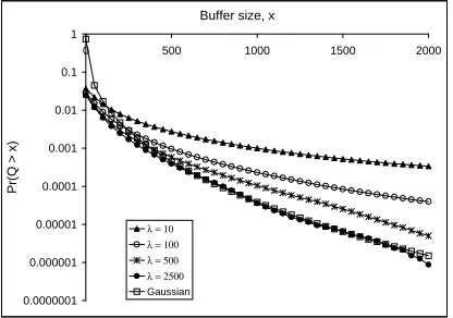
Figure 1 shows an example in which this Gaussian con-vergence occurs. In the figure we see a family of PPBPs, all with µ EAn
100, σ
2
14400 and H 0
8 but with differing levels of aggregation, which are fed into SSQs with service rate C 350
The infinite buffer overflow probabilities for each process are evaluated by simulation. As the value of
λ increases the queueing performance improves, until a rea-sonable approximation of Gaussian performance is achieved. Along the way, however, lower values ofλ produce different queueing performance results for PPBPs with the same values of EAn
, σ
2 and H. In this figure, the Gaussian results are generated by applying Equation (9) to calculate the queueing performance of a Gaussian process having the same variance function as the family of PPBPs considered. We note that in [5] this expression was found to over-estimate the probability of overflow for smaller queue lengths, but the tail behaviour for larger queue lengths corresponds well with that observed in a simulated Gaussian process.
straight-0.0000001 0.000001 0.00001 0.0001 0.001 0.01 0.1 1
0 500 1000 1500 2000
Buffer size, x
Pr(Q > x)
[image:6.595.72.280.60.206.2]λ = 10 λ = 100 λ = 500 λ = 2500 Gaussian
Fig. 1. Convergence of PPBP to Gaussian.
forward Gaussian analytic techniques. In this section we examine more accurate analytic techniques.
An approximation for the queueing performance of the PPBP which is labelled the quasi-stationary approximation was introduced in [3]. Whereas the bounds given above are valid as x? ∞, the quasi-stationary estimate gives an estimate which is valid for λ? ∞. This estimate is more useful for lower values of the buffer threshold x, and has been shown in [3] to give accurate estimates of the infinite buffer queue length distribution for the PPBP SSQ.
The quasi-stationary approximation is based on dividing the PPBP into slowly moving and quickly moving parts. The combined effect of these two components will give the overall queueing performance.
If we consider the PPBP over any such interval of length
W , i.e., the period &t
t W
$, for arbitrary t, then any of the initial bursts which last for the entire time period we label as
long bursts. All other bursts are called short bursts. The short
bursts include: (1) those bursts that start at or before t and end before t W , (2) those bursts that start after t and finish at or after t W and (3) those bursts that start after t and finish at or before t W . Considering these long and short bursts, we will divide the PPBP into two independent processes: (1) the long
bursts process and (2) the short bursts process. The long bursts
process is a stationary but non-ergodic process containing only the long bursts. The short bursts process contains all the remaining bursts, and is stationary on the interval &0
W$ (see
[3]).
By definition, the long bursts process will have constant rate over the interval of length W . This constant rate will be given by nr, where n is the number of long bursts, and r is the rate per burst. The number of long bursts, n, is Poisson distributed with meanλEd
Pr
ω W
where Pr ω x
is the complementary distribution function of the forward recurrence time of the Pareto burst distribution, and is given by Equation (2).
For a given W , we can use known techniques for SRD processes (e.g. the techniques given in [5] or [11]) to calculate the performance of the short bursts process in a queue with
service rate C nr. We then calculate an estimate of the
performance of the PPBP in a queue with service rate C by summing these estimates, weighted by the probability that the long bursts process will contain n bursts.
There are various ways of modeling the queueing behaviour of the short bursts process. One way which is convenient is to model this process as Gaussian. This modeling allows us to apply the formula of [5] to the short bursts process. This formula is summarised in Section V. This approximation is asymptotically accurate as λ? ∞, because for larger λ the short-range dependent process becomes more and more similar to Gaussian.
In order to calculate the queueing performance of the short bursts process, using the Gaussian formula given in Equation (9) we must calculate the value t9
x. t9
x will depend upon the mean and the variance-time curve of the short bursts process. These values will differ from the equivalent expressions for the overall PPBP. The mean of the short bursts process is
mW
rλδγ
γ 1
γδ1 γ
W1 γ
and its variance-time curve is
vst
Var&Aˆt$ t
2r2λW
1 γ
γ 1
0 t W
(11)
The values of t9
x used in the Gaussian formula are restricted to be less than W , so we do not define the variance-time curve of the short bursts process for t W . If no solution to Equation (10) can be found in the range 0 t W then t
9
x W . The final estimate of PrQ x
for the PPBP will depend upon the choice of W . Whatever the value of W , the quasi-stationary estimate is a lower bound on the performance of the PPBP. Therefore, the best estimate of the PPBP performance is produced by choosing W to be the value which maximizes the quasi-stationary estimate of PrQ x
. VII. FITTING THEPARAMETERλ
For any given traffic trace, we wish to automatically cal-culate the parameters of the PPBP such that: (1) the mean and autocorrelation function of the PPBP will be close to those of the real trace and (2) if both are fed into infinite buffer single server queues with the same service rate, they will give almost the same overflow probability curves. This matching of the overflow probability should occur for any buffer threshold and for any service rate. Henceforth we will call such a PPBP a PPBP which fits the real data. Our real trace is a sequence of N consecutive measurements of the amount of traffic originating from the source in consecutive fixed size time intervals, which form a sequence of values
Sn: 1 n N
. From the sequence
Sn we can estimate values for the mean, variance and Hurst parameter. Standard estimators are used to evaluate the mean and variance of the measured streams, and we have used the Matlab imple-mentation of the Abry-Veitch wavelet estimator [1] available from the website http://www.emulab.ee.mu.oz.au/˜darryl/
sec-ondorder code.html to estimate the Hurst parameter of the
streams.
variance and Hurst parameter values identical to those of the measured stream. We have seen in Section V that different members of this family of PPBPs will behave very differently in identical queueing scenarios. The different members of the family are differentiated by their different values of λ, so choosing the correct value for λ would appear to be vital to producing a model which accurately reflects reality.
We define λ9 to be the value of the Poisson parameter which produces a PPBP which fits the real data. This fitting is determined though a matching of the complementary queue length distributions within infinite buffer SSQs for a single fixed service rate C and a range of buffer thresholds.
By feeding the sample values
Sn through an infinite buffer SSQ with service rate C we calculate the complementary queue length distribution for the sample values. We calculate the proportion of time when the amount of work stored in the infinite buffer exceeds a given threshold for a set of buffer thresholds,
xi: 0 i M 1
. Typically we consider evenly spaced buffer thresholds, xi i∆xwhere∆xis a positive constant, but the xivalues may be any set of non-negative reals. The overflow probabilities calculated in this way form the set
pi PrQ xi
.
We search for the value of λ9 which, together with the other three fitted parameters, namely, the mean, the variance and the Hurst parameter, defines a PPBP which fits the real trace. In the following sections we examine the fitted PPBP by generating queue length distributions for SSQs with service rates that are different from the value of C used in calculating λ9
We also compare the marginal distribution and autocorrelation function of the PPBP with those of the measured traffic trace.
To findλ9 we must consider a family of PPBPs. All PPBPs in this family will be fitted to the values of mean, variance and Hurst parameter measured in the set of values
Sn and
all will have the same values for δ and γ. For each value of
λ considered, we use the quasi-stationary estimate developed in [3] and summarised above in Subsection VI to estimate the queueing performance of this PPBP in an infinite buffer SSQ with the same service rate, C
as the SSQ used in calculating the pivalues. Overflow probabilities are estimated for the same values of xi to give a set of values
eiλ
PrQ xi
. For each value ofλwe calculate a measure of the difference between the estimated values,
eiλ
and the values given by the data,
pi . To do this, we divide the results into two groups, depending upon the relative size of eiand pi. If ei! pi then we assign xito the set X . Otherwise, we assign xi to the set ¯X .
We then calculate two sums:
G1λ
∑
xi X
log pi log eiλ
2 (12)
and
G2λ
∑
xi X¯
log pi log eiλ
2
(13)
We define the overall accuracy of the model in predicting
the behaviour to be
Gλ
G1λ @ G2
λ
(14)
We assume that the optimal value forλ9 occurs when Gλ
0. It is possible that there will be more than one value of
λ for which Gλ
0. We know that the quasi-stationary approximation is valid for λ? ∞, so in this case we take the largest λ for which Gλ
0 to be λ9, on the grounds that this will be the most reliable of the possible solutions. Alternatively, if there is no value of λ for which Gλ
0
thenλ9 is the value ofλ which minimizes AGλ
A.
An alternate measure for the accuracy of the model could be given by GSλ
G1λ B G2
λ . GS
λ
is the sum of the squares of the distances (on a logarithmic scale) between the two set of values
eiλ
and
pi , and so λ9 could be found by minimizing GSλ
, i.e. using a minimum mean square error technique to findλ9 . We have chosen not to use this technique, as the differential measure Gλ
varies more quickly in the region of interest, and therefore provides a more precise estimate for λ9. We expect that the values of
λ9 given by solving Gλ
0 will be similar to those yielded by minimizing GSλ
in most cases.
VIII. PREDICTING THEQUEUEINGPERFORMANCE In Figure 2 we show that the PPBP also successfully predicts the queueing performance of an IP traffic stream. This IP traffic stream is derived from link traffic recorded as a sequence of IP packet header summaries. This packet header data was reduced to a sequence of integers, where each value represents the number of bytes transmitted on the link in a 0.1 second interval. For this sequence, we measured a mean arrival rate of 5225 bytes per interval, a variance of 21
223C 10
6and H
6 0
91. The fitting of the parameterλ is carried out using the method described in Section VII for a service rate of C 21000 (bytes per 0.1 s) with a family of PPBPs with γ 1
18 and δ 1. The fitting process gives a level of aggregation of λ 0
267
The figure shows queueing performance for a service rate of
C 21000 bytes per 0.1 second. The confidence intervals for the λ 0
267 simulation results are approximately the same size as the marks used to indicate the points, and so are omitted from this figure.
We observe that the Gaussian process with the same cor-relation function as the PPBPs shown considerably under-estimates the loss levels experienced by the real traffic. This suggests that, even though this IP link is likely to be carrying traffic from a relatively large number of independent sources, the link traffic is still far from being sufficiently aggregated for a Gaussian model to be applicable.
0.000001 0.00001 0.0001 0.001 0.01 0.1 1
0 20000 40000 60000 80000 100000
Buffer threshold, x (packets)
Pr(Q > x)
IP Trace λ = 0.267
λ = 2.6 λ = 26
[image:8.595.73.280.58.205.2]Gaussian
Fig. 2. Matching the PPBP to an IP trace
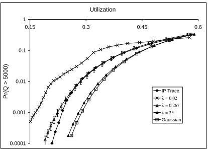
0.0001 0.001 0.01 0.1 1
0.15 0.3 0.45 0.6
Utilization
Pr(Q > 5000)
IP Trace
λ = 0.02 λ = 0.267 λ = 25
Gaussian
Fig. 3. Comparison of queueing performance for a range of utilizations.
those shown in Figure 2, we can see that the PPBP accurately predicts the performance of the IP data stream in SSQs, for a wide range of buffer sizes and service rates.
Figure 3 presents an examination of the impact of changing service rates. Here we have chosen a single value of the buffer threshold, x 5000 bytes, and examined the values of PrQ
x for a range of service rates. Qualitatively similar results are obtained for other fixed buffer size values.
For low service rates, i.e. high utilizations, the probability of loss is quite high, and all values ofλgive acceptable estimates of the loss. In fact even the Gaussian process gives reasonable estimates of queueing performance for utilizations above 0
6. As the service rate is increased (and the utilization decreases) the choice ofλbecomes more significant. Figure 3 shows that a single value of λgives a good fitting for a range of service rates. For example,λ 0
267 produces a PPBP which predicts the queueing behaviour of the IP stream well for levels of utilization greater than 20%, corresponding to service rates of
C 25000 bytes per 0.1 second interval, or lower. The results shown in Figure 2 fall within this region whereλ 0
267 gives a good approximation of the performance of the IP trace.
Looking at Figure 3 in conjunction with Figure 2 we can see that the PPBP correctly predicts the queueing performance of
the real traffic across a wide range of service rates and buffer sizes.
We have achieved this by matching just three measurable properties of the original stream, and then setting a fourth parameter. The setting of the fourth parameter, λ9 , is made with respect to results for a given service rate, but we see here that this fitting is good for a range of service rates. Thus the PPBP meets our main criteria as a simple and accurate model for IP traffic.
IX. MATCHING THESTATISTICS
We recall that along with a matching of the queueing performance of the real traffic, it is also desirable that the model match the first and second order statistics of the modeled traffic. In this section, we evaluate the ability of the PPBP to achieve this. We use the same PPBP fitted to the IP trace as in Section VIII.
Figure 4 shows a Q-Q plot which gives a comparison between the marginal distribution of the original IP trace and that of a PPBP which is correctly fitted to the trace. The Q-Q plot is formed by placing a point x
y where Pr
X x
PrY y
, in which X has the distribution of the IP trace and Y has the distribution of the model. As shown in Section VIII, the PPBP fitted to the trace hasλ 0
267. The marginal distribution of the PPBP was measured from 60 simulations of one million samples each. We see that the PPBP matches marginal distribution of the IP trace reasonably well, although not perfectly.
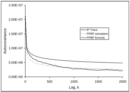
Figure 5 shows a comparison between the autocovariance of the original trace and that of a PPBP fitted to the trace. In this case, 60 sets of one million samples each are averaged to generate the simulation results. For comparison, the ACF calculated analytically based on Equation (3) is also shown. The finite duration of the simulations (making extremely rare events unlikely to occur) is the most likely explanation for the fact that the simulation results show covariances lower than those predicted by the theory. Since the IP trace is also finite, the good match between the IP trace and the simulations is the appropriate indicator of a successful model and the results depicted in Figure 5 are quite pleasing.
We note that our method of fitting a family of PPBPs to a given traffic stream means that the autocovariance function will not be altered by changes in the value ofλ. Thus we may conclude that the changes in queueing performance caused by changes in the value ofλoccur primarily because of changes in the marginal distribution. This leads us to interpretλ as a measure of the distance between the marginal distribution of the traffic stream and a Gaussian distribution.
[image:8.595.72.279.249.397.2]0 5000 10000 15000 20000 25000 30000
0 5000 10000 15000 20000 25000 30000
IP Trace
[image:9.595.335.542.59.204.2]PPBP
Fig. 4. Q-Q plot comparing the IP trace with the fitted PPBP.
0.00E+00 5.00E+06 1.00E+07 1.50E+07 2.00E+07 2.50E+07
0 500 1000 1500 2000
Lag, k
Autocovariance
IP Trace PPBP simulation PPBP formula
Fig. 5. Autocovariance of the trace and the fitted PPBP.
X. OPTICALINTERNETIMPLICATIONS
We have shown that the PPBP has all the attributes of an accurate Internet traffic model. Using this model, we are now able to confirm the view of [2] and [21] that the long-range dependent (LRD) phenomenon observed in Internet traffic [10], [14] does not necessarily lead to low utilization. Although the traffic does not smooth out as voice traffic did, it will smooth out eventually due to heavy multiplexing.
In particular, we used the IP traffic trace of Section VIII that was taken in 1998 on a certain US link (this trace was also used in [3] and [19]). We first use the PPBP model of this traffic trace as obtained above, and then consider several different PPBP processes each of which is a process resulting from multiplexing together a number of statistical copies of the original PPBP model of the trace. Recall that multiplexing of a number of PPBPs gives another PPBP. For each of these PPBP processes, we used the quasi-stationary approximation to estimate packet loss in a zero buffer SSQ, and determined the capacity required to guarantee a given low packet loss. We show the results in Figure 6. For the original traffic stream, we needed to run the system at 15% utilization to obtain 1/1,000,000 loss probability, however, if it is multiplexed 500 times, we obtain 80% utilization. (Notice
0 0.1 0.2 0.3 0.4 0.5 0.6 0.7 0.8 0.9
0 100 200 300 400 500
M
Utilization
[image:9.595.71.278.59.206.2]Year1998 2004 2005 2006 2007
Fig. 6. Improving utilization as multplexing levels increase.
that future Internet traffic may have different characteristics than current traffic, however, it is expected that future traffic will include large components of real-time services, which in fact generate smoother streams.) Given the growth of the Internet, we estimate that it would take nine years to achieve this level of multiplexing for this particular link. However, we do not have to wait another five years to observe it. The smoothing out of Internet traffic has already been confirmed by measurements in [21] and references therein. This smoothing out of Internet traffic phenomenon makes the bufferless optical Internet very appealing.
XI. CONCLUSIONS
In this paper we have examined the PPBP as a model for Internet traffic, and we have found it to be very promising in this role. We have shown that the PPBP meets our criteria for a simple and accurate traffic model. We have used the PPBP to predict future multiplexing and link efficiency levels. We have demonstrated that there is evidence that the future optical Internet will be efficient despite the facts that it will be bufferless.
ACKNOWLEDGMENT
The authors wish to thank Danielle Liu of AT&T for supplying the IP packet trace analyzed in this paper.
REFERENCES
[1] P. Abry and D. Veitch, “Wavelet analysis of long-range-dependent traffic,” IEEE Transactions on Information Theory, vol. 44, no. 1, pp. 2–15, Jan. 1998.
[2] R. G. Addie, M. Zukerman, and T. D. Neame, “Broadband traffic modeling: Simple solutions to hard problems,” IEEE Communications Magazine, vol. 36, no. 8, Aug. 1998.
[3] R. G. Addie, T. D. Neame, and M.Zukerman, “Performance evaluation of a queue fed by a poisson pareto burst process,” Computer Networks, 2002.
[4] R. G. Addie, “On the weak convergence of long range dependent traffic processes,” Journal of Statistical Planning and Inference, vol. 80, pp. 155–171, 1999.
[image:9.595.71.279.248.396.2][6] J. Beran, R. Sherman, M. S. Taqqu, and W. Willinger, “Long-range-dependenceD in variable-bit-rate video traffic,” IEEE
Transac-tions on CommunicaTransac-tions, vol. 43, no. 2/3/4, pp. 1566–1579, Febru-ary/March/April 1995.
[7] J. Choe and N. B. Shroff, “A central limit theorem based approach to analyze queue behavior in ATM networks,” IEEE/ACM Transactions on Networking, vol. 6, no. 5, pp. 659–671, Oct. 1998.
[8] D. R. Cox and V. Isham, Point Processes, Chapman and Hall, 1980. [9] M. E. Crovella and A. Bestavros, “Self-similarity in world wide web
traffic: Evidence and possible causes,” IEEE/ACM Transactions on Networking, vol. 5, no. 6, pp. 835–846, Dec. 1997.
[10] A. Feldman, A. C. Gilbert, W. Willinger, and T. G. Kurtz, “The changing nature of network traffic: Scaling phenomena,” Computer Communication Review, vol. 28, no. 2, pp. 5–29, Apr. 1998.
[11] P. W. Glynn and W. Whitt, “Logarithmic asymptotics for steady-state tail probabilities in a single server queue,” Journal of Applied Probability, vol. 31, pp. 131–156, 1994.
[12] K. Kobayashi and Y. Takahashi, “Tail probability of a Gaussian fluid queue under finite measurement of input processes,” in Performance and Management of Complex Communication Networks, T. Hasegawa, H. Takagi, and Y. Takahashi, Eds., pp. 43–58. Chapman & Hall, 1998. [13] M. M. Krunz and A. M. Makowski, “Modeling video traffic using M/G/∞input processes: A compromise between Markovian and LRD models,” IEEE Journal on Selected Areas in Communications, vol. 16, no. 5, pp. 733–748, June 1998.
[14] W. E. Leland, M. S. Taqqu, W. Willinger, and D. V. Wilson, “On the self-similar nature of Ethernet traffic (extended version),” IEEE/ACM Transactions on Networking, vol. 2, no. 1, pp. 1–15, 1994.
[15] N. Likhanov, B. Tsybakov, and N. D. Georganas, “Analysis of an ATM buffer with self-similar (”fractal”) input traffic,” in Proceedings of IEEE Infocom ’95, 1995.
[16] H. W. Lilliefors, “On the Kolmogorov-Smirnov test for normality with mean and variance unknown,” Journal of the American Statistical Association, vol. 62, pp. 399–402, 1967.
[17] B. Maglaris, D. Anastassiou, P. Sen, G. Karlsson, and J. Robbins, “Performance models of statistical multiplexing in packet video com-munications,” IEEE Transactions on Communications, vol. 36, pp. 834– 844, July 1988.
[18] O. Narayan, “Exact asymptotic queue length distribution for fractional Brownian traffic,” Advances in Performance Analysis, vol. 1, no. 1, pp. 39–63, 1998.
[19] T. D. Neame, M. Zukerman, and R. G. Addie, “Applying multiplexing characterization to VBR video traffic,” in Proceedings of ITC 16, June 1999.
[20] I. Norros, “On the use of fractional Brownian motion in the theory of connectionless networks,” IEEE Journal on Selected Areas in Communications, vol. 13, no. 6, pp. 953–962, Aug. 1995.
[21] A. M. Odlyzko, “The Internet and other networks: Utilization rates and their implications,” Information Economics & Policy, vol. 12, pp. 341–365, 2000.
[22] M. Parulekar and A. M. Makowski, “Tail probabilities for M/G/∞ processes (I): Preliminary asymptotics,” Queueing Systems - Theory and Applications, vol. 27, pp. 271–296, 1997.
[23] V. Paxson and S. Floyd, “Wide-area traffic: The failure of Poisson modeling,” IEEE/ACM Transactions on Networking, vol. 3, no. 3, pp. 226–244, 1995.
[24] J. Roberts, U. Mocci, and J. Virtamo, Eds., Broadband Network Teletraffic, Final Report of Action COST 242, Springer, 1996. [25] K. P. Tsoukatos and A. M. Makowski, “Heavy traffic limits associated
with M/G/∞input processes,” Queueing Systems, vol. 34, no. 1–4, pp. 101–130, 2000.
[26] B. Tsybakov and N. D. Georganas, “On self-similarity in ATM queues: Definitions, overflow probability bound, and cell delay distribution,” IEEE/ACM Transactions on Networking, vol. 5, no. 3, pp. 397–409, June 1997.
[27] B. Tsybakov and N. D. Georganas, “Self-similar traffic and upper bounds to buffer-overflow probability in an ATM queue,” Performance Evaluation, vol. 32, pp. 57–80, 1998.
[28] B. Tsybakov and N. D. Georganas, “Overflow and losses in a network queue with a self-similar input,” Queueing Systems, vol. 35, pp. 201– 235, 2000.
[29] B. Tsybakov and N. D. Georganas, “Self-similar processes in commu-nications networks,” IEEE Transactions on Information Theory, vol. 44, no. 5, pp. 1713–1725, September 1998.