We can still learn about probability by rolling dice and tossing coins

We Can Still Learn About Probability By Rolling Dice And Tossing Coins

KEYWORDS Probability; Teaching; Dice; Coins

Peter K Dunn

Department of Mathematics and Computing, University of Southern Queensland, Toowoomba, Australia e-mail: [email protected]

Summary

Rolling dice and tossing coins can still be used to teach probability even if students know (or think they know) what

happens in these experiments. Many simple variations of these experiments are considered which are interesting, potentially enjoyable and challenging. Using these variations can cause students (and teachers) to think again about the statistical issues involved—and learn in the process.

INTRODUCTION

Rolling dice and tossing coins often form part of the staple diet of basic statistics and probability lessons. In this paper, we show how even these well-tried and digested experiments can still provide much food for thought in mathematics classes by making simple variations to these experiments.

Truran (1984) has shown that, in children under ten, many basic probability concepts based on using dice and coins are misunderstood. Green (1983) and Kerskale (1974) also showed that young children have difficulty in ascribing equal probabilities to each face of a die. In addition, they showed that this was more likely to occur in students with an inferior reasoning ability, and that students generally “improved” as they got older. Hawkins and Kapadia (1984) show that children can and do learn probability concepts, and consider

many interesting questions concerning the way children learn, and are taught, probability.

experiments that make them so popular: They are experiments that are easily understood and performed by everyone, are avenues for easy and quick data collection, and the data are easily analysed.

ROLLING DICE

In this section, we particularly focus on rolling dice. Historical data and numerous variations are discussed. Note that we do not discuss any regular k

-sided dice, since essentially any discussion is a naive variation of the standard six-sided dice.

History

Some people have kept records of vast numbers of dice rolls. Hand, Daly, Lunn, McConway and Ostrowki (1996) give the famous Wolf data, in which Wolf recorded the frequency that each face appeared in 20 000 rolls of a die; see Table 1. This is useful for discussing fundamental statistical issues such as variability and randomness.

One question that presents itself is whether the die is biased, since a 4 showed up relatively rarely (and a 2 relatively often). The expected proportion is 1/6 = 0.167; is the difference of importance? How could we find out?

These questions may appear simple, but they are fundamental for understanding statistics. They can give the student an appreciation of the concept of sampling variability—in my experience one of the most difficult concepts in statistics, yet the very basis of its existence.

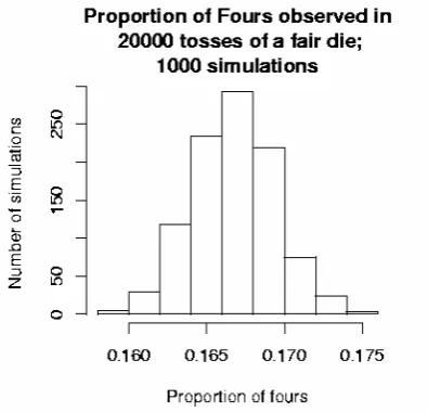
The standard solution to the question is an hypothesis test. An alternative that the students may enjoy is to use a computer simulation to “roll” a die 20 000 times and record the proportion

of fours. After doing this 1000 times, 1000 proportions will be found, from which a histogram of the proportion of fours can be constructed; see Figure 1. This suggests that a proportion as low as 0.1458, as seen in the data, appears very rarely (and 2 very often); quite possibly the die was biased, or Wolf rolled badly—20 000 times!

Table 1: Wolf's data: The number of times each face shows in 20 000 rolls of a die. (Source: Hand et al., data set 131)

Face Frequency Proportion

1 3407 0.1704 2 3631 0.1816 3 3176 0.1588 4 2916 0.1458 5 3448 0.1724 6 3422 0.1711

Another historical data set is Weldon’s dataset (see Hand et al. data set 263).

Weldon rolled twelve dice 26306 times in the 1800s. Various subsets of the outcomes were studied and reported.

Figure 1 A histogram of the proportion of fours in 20000 rolls of a die (after 1000 simulations)

Efron’s dice

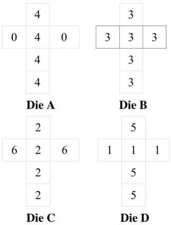
consist of four cubes as shown in Figure 2. The interesting property of Efron’s dice is that: P(A beats B)= 2/3; P(B beats C)= 2/3; P(C beats D)= 2/3; and yet P(D beats A)= 2/3. This is almost always unexpected and can be used to pique some curiosity.

4 3

0 4 0 3 3 3

4 3

4 3

Die A Die B

2 5

6 2 6 1 1 1

2 5

2 5

Die C Die D

Figure 2 Efron's dice: With these dice, A beats B, B beats C, C beats D and D beats A, all with probability 2/3.

It is also simple to demonstrate the probabilities of one die beating the other as given above; see Table 2. In this way, the students can check the teacher’s assertions! An evocative way of studying the probabilities is to play a game with the teacher versus the class; almost invariably, students initially won’t believe that D beats A if A beats B, B beats C and C beats D. Rouncefield and Green (1989) discuss some other sets of dice with similar properties.

Table 2: Die A vs Die B in Efron's dice: A tick means that Die A beats Die B, so that P(A beats B)=2/3. Note that this implies each face on each die is equally likely to occur.

Die A

0 0 4 4 4 4 3 X X √ √ √ √ 3 X X √ √ √ √ 3 X X √ √ √ √ 3 X X √ √ √ √ 3 X X √ √ √ √

Die B

3 X X √ √ √ √

Biased dice

Gelman and Nolan (2002) use a simple class experiment to create biased die. They give small groups of students a wooden die and a piece of sandpaper and ask the students to alter the die, however they want, to make it biased in some way. Gelman and Nolan report that a large amount of sanding is generally needed before an appreciable difference is made. See Gelman and Nolan (2002) for more details of this experiment.

This activity is of great interest to the students as they have the opportunity to create a biased die. Many also see the activity as a competitive challenge: they seem to believe they can do this well, and can be creative in how they approach the task. An important discussion can then centre on how to

know if the die is biased in the presence

of sampling error.

An interesting variation of this experiment is to present the students with five dice, only one of which is (not obviously) biased, and have them determine which it is.

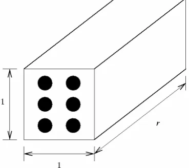
Dice of dimension 1 x 1 x r

constructed a set of dice of size 1 x 1 xr

(see Figure 3) where r can be considered

the aspect ratio of the die. The probabilities of rolling a 6 are to be determined (note that a 6 is on both 1 x 1

faces). This problem is very easy to state, but it is not at all clear what the probabilities will be. There are some special cases for which the probabilities are known, however:

1. As r approaches 0, P(6 is rolled)

approaches 1;

2. As r approaches infinity, P(6 is

rolled) approaches zero;

3. When r = 1, P(6 is rolled) = 1/3.

In one of my classes, one student suggested a formal solution: The probability of obtaining a 6 might be related to the ratio of the surface areas. The total surface area is 2 + 4r, so the

probability of obtaining a 6 then might be 2/(2 + 4r) = 1/(1 + 2r). Interestingly,

the shape of this graph is certainly not correct even though it satisfies the three conditions above.

Figure 3: A non-symmetric die of size 1 x 1 x r. Note that both 1 x 1 faces are labelled as a six.

It is also interesting to note that a graph of P(6 is rolled) versus r is not

symmetric about r = 1, since the

probability of obtaining a 6 then is 1/3,

which is not halfway between the limits of 0 and 1.

As with the biased dice above, a simple experiment can be devised in which students can estimate the probability of rolling a 6 for various values of r. A

number of statistical issues can be addressed in this experiment:

• What values of r should we use,

and why?

• How many times should we roll each die of side r?

• Should there be a different number of rolls depending on r?

Explain!

• What other factors might affect the answers besides the value of

r?

• How should the data be reported?

• What steps should be taken to conduct the experiment? (Talk about experimental design and protocol.)

• How should the dice be rolled? Each of these questions is, to some extent, open-ended, which students either love or loathe. They cover a surprisingly broad range of statistical topics. Answers to the questions will probably vary widely across the class, and oftentimes the answers are based on what is practical more than what is statistical (for example, the values of r to

use depends on what dice I have with me!). But important statistical concepts are discussed in this simple to understand, simple to perform experiment.

Table 3: The results of rolling a 1 x 1 x r die 760 times for various aspect ratios, r.

Aspect ratio P(roll a 6) Aspect ratio P(roll a 6)

0.25 0.98 1.10 0.25 0.50 0.80 1.15 0.24 0.75 0.61 1.25 0.18 0.85 0.52 1.50 0.06 0.90 0.47 1.75 0.03 1.00 0.33 2.00 0.02

As an aside, the relationship between the ratio r and the probability of rolling a 6

has been explored in one of my classes using more advanced statistical techniques; details can be found in Dunn (2003).

Establishing a protocol for rolling

Some experiments were briefly described above for estimating the probabilities of rolling given outcomes. It should be made clear that certain protocols need to be established first to ensure consistency throughout the experiments. Both Gelman and Nolan (2002) and Dunn (2003) discuss this more fully. Rolling techniques, for example, can play a large part in determining the outcome of the experiments. Gelman and Nolan (2002) demonstrate this to the students before the students start their experiments.

TOSSING COINS

In the last section, variations to the standard die rolling experiment were considered. Similarly, variations to the tossing coins experiment can also be used. First, some historical data are considered.

History

Three historical examples of coins being tossed are given in Moore (2003, p 225):

1. Count Buffon tossed a coin 4040 times for 2048 heads, a proportion of 0.5069;

2. Karl Pearson tossed a coin 24000 times for 12012 heads, a proportion of 0.5005;

3. John Kerrich tossed a coin 10000 times for 5067 heads, a proportion of 0.5067.

All the results are close to the expected proportion of 0.5; interestingly, all the

proportions are greater than 0.5. A simulation study, as used with the dice, could be used to assess these results.

More recently, the introduction of the Euro into Europe provided an opportunity to examine the potential bias in the new currency. Students at the Akademia Podlaska in Poland spun a

Belgian one-Euro coin 250 times are recorded 140 heads (see Gelman and Nolan, 2002). This received much press coverage, including its implications for sporting events whose start often depends on the toss of a coin. The

commentaries seemed to miss the subtle differences between tossing and spinning a coin. The next section explores this further.

Methods of determining the probability of a head

It has already been noted that the method used for rolling dice is important; it is no less important for “tossing” coins. There are at least four (straightforward) ways of determining the probability of a head:

well, the coin will do a large number of turns in the air and land randomly.

2. Coins can be rested on their edge on a table, and the table thumped. The coin will fall to show heads or tails.

3. Coins can also be spun. The coin can be held upright between your forefinger and the table, and then spun with the other forefinger. Then slap your hand onto the coin and see which side is face up.

4. Coins can be rolled on a flat surface until they fall onto one side (usually after spiralling). A comparison of the four methods can be constructive and can open the door to many fruitful discussions. Anecdotal evidence suggests the probability of a head is not the same for all methods. For further discussion, see Humble (2001) where the author provides a mathematical discussion of the physics of spinning and rolling coins.

Tossing thumbtacks

Tossing coins is convenient; but other items can also be tossed. Why not examine the probability of a thumbtack landing point-up? (Some of the other methods are not suitable for other objects; don’t whack your hand on a thumbtack for example!) Or examine the probability that a bottle top will land open-side up? As a boy, we often tossed cricket bats to see who would bat or bowl first; what are the relative probabilities? Not surprisingly, these probabilities are not necessarily a half (though actual probabilities will depend on the type of thumbtack, bottle top or cricket bat used).

Try to bias a coin

Gelman and Nolan (2002) discuss an experiment in which their students are

encouraged to try and bias a coin. They are provided with a plastic checker and a piece of plasticine; the aim is to maximize the chance of tossing a “head”. See Gelman and Nolan (2020) for more details. They report that

spinning a doctored checker can

appreciably change the chance of a “head” appearing, but the same is not seen when the checker is tossed. In one

example, one student’s checker landed “heads” 23 times out of 100 spins; the

same checker landed “heads” 53 times out of 100 tosses.

DISCUSSION

The old favourite statistical experiments of rolling dice and tossing coins are wonderful classroom experiments: they are quick and simple to do, explain and analyse. But they have the potential to be boring; students know (or at least think they know) what happens when

coins are tossed and dice are rolled. We have discussed some variations of these classic experiments that can restore some fun and challenges, without compromising on the simplicity that has made them appealing.

Some simple classroom activities were discussed; numerous others can also be developed. The answers to many of these questions are, of course, not easy. But getting the answer is not as important as the discussion and understanding that the questions initiate.

References

Dunn, Peter K. (2003). What happens when a 1 x 1 x r die is rolled? The

American Statistician. 57, 258–264.

Green, D. R. (1983). Shaking a six. Mathematics in school, 12, 29–32.

Hand, D. J., Daly, F., Lunn A. D., McConway, K.J. and Ostrowski, E. (1994). A Handbook of Small Data Sets. London: Chapman and Hall.

Hawkins, A. S., and Kapadia, R. (1984). Children's conceptions of probability: a psychological and pedagogical review. Education Studies in Mathematics, 15, 349–377.

Humble, S. (2001). Rolling and spinning coin: A level gyroscopic processional motion. Teaching Mathematics and its Applications. 20, 18–24.

Kerslake, D. (1974). Some children's views on probability. Mathematics in School, 5, 22.

Moore, D. S. (2003). The Basic Practice of Statistics (3rd ed.). New York: WH Freeman and Co.

Rouncefield, M. and Green, D. (1989). Condorcet's Paradox. Teaching Statistics, 11, 46–49.