This is a repository copy of
Species reintroduction and community-level consequences in
dynamically simulated ecosystems
.
White Rose Research Online URL for this paper:
http://eprints.whiterose.ac.uk/117770/
Version: Published Version
Article:
Byrne, Justin G.D. and Pitchford, Jonathan W. orcid.org/0000-0002-8756-0902 (2016)
Species reintroduction and community-level consequences in dynamically simulated
ecosystems. Bioscience Horizons. hzw009. ISSN 1754-7431
https://doi.org/10.1093/biohorizons/hzw009
[email protected]
https://eprints.whiterose.ac.uk/
Reuse
This article is distributed under the terms of the Creative Commons Attribution-NonCommercial (CC BY-NC)
licence. This licence allows you to remix, tweak, and build upon this work non-commercially, and any new
works must also acknowledge the authors and be non-commercial. You don’t have to license any derivative
works on the same terms. More information and the full terms of the licence here:
https://creativecommons.org/licenses/
Takedown
If you consider content in White Rose Research Online to be in breach of UK law, please notify us by
. . . .
. . . .
. . . .
Research article
Species reintroduction and community-level
consequences in dynamically simulated
ecosystems
Justin G.D. Byrne* and Jonathan W. Pitchford
Department of Biology, University of York, York, North Yorkshire YO10 5DD, UK
*Corresponding author:Department of Biology, University of York, York, North Yorkshire YO10 5DD, UK. Tel:+44 01904 328 633. Email: [email protected]
Supervisor:Dr Jonathan W. Pitchford, Department of Biology, University of York, York, North Yorkshire YO10 5DD, UK.
Global biodiversity, and its associated ecosystem services, are threatened due to species extinctions. Reintroducing locally extinct species may be a partial solution to this problem. However, the success and possible consequences of any artificial reintroduction will depend on its ecological community, and the reaction of that community to the species’extinction and reintroduction. Mathematical models can offer useful insights by identifying the key features of communities and reintro-duced species most likely to result in successful reintroductions.
Here we simulated extinctions and reintroductions for a range of theoretical food webs generated using an estab-lished bioenergetics model. This allows the probability of successful reintroductions to be quantified as a function of two important ecological factors: the connectance of the food web, and of the time between extinctions and reintroductions.
Reintroduction success is measured across an ensemble of 1796 simulated communities, with connnectances of 0.05, 0.15 and 0.3, using three criteria: presence of the reintroduced species in thefinal community, unchanged species richness in the
final community compared to the pre-extinction persistent community and the complete restoration of the community (including both species richness and equilibrium biomass distributions).
Although only 12 reintroduced species fail to re-establish according to minimal criteria, the process of extinction and reintroduction frequently has a large effect on the community composition. Increasing time to reintroduction increases both the probability of species loss, and equilibrium biomass change in the community. Proportionally, these community-level impacts occur more frequently when the reintroduced species is a primary producer or top predator. These results indicate that ignoring broader measures of reintroduction success could seriously underestimate the impact of reintroductions on the ecological community. These quantitative results can be compared to empirical literature and may help reveal which fac-tors are most important to the success of reintroductions.
Key words:extinction, food web, niche model, nonlinear bioenergetic dynamic model, reintroduction, connectance
Introduction
Biodiversity loss and the science of
reintroduction biology
Global biodiversity loss is a well-documented phenomenon that threatens ecosystems worldwide. There is strong evidence that biodiversity is positively correlated with certain ecosys-tem services (Cardinaleet al., 2012). Reintroductions, defined as ‘the intentional movement and release of an organism inside its indigenous range from which it has disappeared’ (IUCN/SSC, 2013), are therefore becoming increasingly attract-ive in conservation.
Seddon, Armstrong and Maloney (2007)detailed the
his-tory of reintroduction biology, dating from the 1907 reintro-duction of American Bison (Bison bison) to Oklahoma. Success stories, such as the reintroduction of Grey Wolves to Yellowstone (Ripple and Beschta, 2012), show that such efforts can benefit an area’s ecology and management. Other issues, such as changing public attitudes to zoos, increased governmental conservation action and a desire to re-establish or restock hunting populations have led to an increase in reintroduction programmes since the 1990s (Seddon, Armstrong and Maloney, 2007).
Despite this practical activity, the science underpinning reintroduction biology is still developing and lacks the mature theoretical framework seen in sisterfields such as invasion biol-ogy (Seddon, Armstrong and Maloney, 2007). Some general rules exist describing, for example, the importance of maintain-ing genetic diversity in reintroduction populations (Renet al., 2014), or using more individuals in reintroduction attempts (Godefroidet al., 2011). However, most work published in the
field is limited to case-by-case predictions (Armstrong and Ewen, 2002;Bennettet al., 2013;Davidson and Armstrong, 2002).
Williams (1997)suggested three stages characterizing the maturation of a science, summarized bySeddon, Armstrong and Maloney (2007)as‘(1) observation guided by intuition, tradition, and guesswork; (2) organization of those observa-tions into coherent categories, the exploration of observaobserva-tions for patterns, and the clear description of patterns; and (3) rec-ognition of the underlying causes of patterns and formulation of theories that lead to testing of predictions deduced’.
Seddon, Armstrong and Maloney (2007) concludes that
reintroduction biology is advancing into stage two, but could progress faster by drawing on theory from other disciplines.
Computer modelling will be important in the development of the science of reintroduction ecology (Armstrong and Seddon, 2008). However, although population viability ana-lysis models can be used in individual reintroduction projects
(Nolet and Baveco, 1996;Seddon, Armstrong and Maloney,
2007), no predictive models of general reintroduction success have been proposed.
Here, we describe a modelling framework to predict the success of reintroductions based on the delay between
extinction and reintroduction, and the trophic identity of the reintroduced species. This method has been adapted from work modelling invasion success (Romanuket al., 2009).
Modelling ecological dynamics
Dynamic network models have been used to describe and quantify many complex biological phenomena, ranging from gene pathways and chemical reactions to climate change and ecological communities (Proulx et al., 2005). Such models have been used in invasion biology to predict invasion success based on general community network and invasion species variables (Romanuket al., 2009). This was accomplished by generating independent realizations of dynamic communities, randomly parameterized from a range of empirically based values using the so-called niche model of generating complex food webs (Williams and Martinez, 2000). These communi-ties were simulated deterministically, using coupled ordinary differential equations (ODEs), following established methods
(Brose, Williams and Martinez, 2006; Williams and
Martinez, 2004;Yodzis and Innes, 1992).
The niche model of generating complex food webs improves upon May’s random model (May, 1972) and Cohen’s cascade model (Cohen, Briand and Newman, 1990). It successfully estimates the central tendency of empirical data better than the other models, and with generally smaller nor-malized errors of the empirical web properties on the means of those properties in the model (Williams and Martinez, 2000).
The bioenergetics model used here is reconstructed from
Romanuk et al.(2009). It incorporates a density dependent functional response in the interspecific feeding relationships (Holling, 1959b). We use a modified type II response, referred to as a‘type II.2’, intermediate between type II and type III responses (Holling, 1959a,b;Williams and Martinez, 2004). The model lacks Allee effects (Courchamp, Berec and Gascoigne, 2008) and stochastic elements; instead its deter-ministic nature allows the general trends underlying reintro-duction success to be identified.
Aims
By modelling extinction and reintroduction, we aimed to answer the following questions:
(i) How does time to reintroduction (the duration between extinction and reintroduction of the subject species) affect the success of reintroductions, as measured accord-ing to three criteria:
(a) Reintroduction subject species re-establishment: is the species present in the community at the end of the experiment?
(b) Successful restoration of the original species richness: does the subject species or other species go extinct? (c) The successful restoration of the equilibrium
bio-masses of all of the community’s species?
. . . .
Research Article Bioscience Horizons•Volume 9 2016
. . . .
(ii) How does web connectance affect the success of reintroductions?
(iii) How does the reintroduced subject species’trophic level affect the success of reintroduction?
(iv) If species are lost from communities during the simulations:
(a) Is there a relationship between the trophic group of the species lost and the trophic group of the reintro-duced species?
(b) When are species lost from communities? Does this happen while the subject species is extinct or is it a consequence of the reintroduction?
Methods
Food webs were generated at three levels of expected directed connectance (C), C= 0.05, C= 0.15 and C =0.3; actual directed connectance was also recorded. Directed connec-tance, the probability that any two species in the food web have a feeding relationship, is equal toL/S2, whereLis the number of feeding relationships between species (S) (Martinez, 1991) and is expected to be similar to the expected connectance in generated webs. Communities with different levels of connectance may react differently in simulations, and therefore data is split by the level of expected connectance during analysis.
Simulations were implemented as follows:
Initially, random food webs were generated using the niche model (Williams and Martinez, 2000) with expectedC
of 0.05, 0.15, or 0.3, as detailed in Appendix 1. Then, each species was assigned an initial biomass drawn from a uni-form random distribution from 0.5 and 1. These were kept identical in all simulations. Each network’s interaction dynamics were simulated using the bioenergetic model until timet=2000, in line with previous work (Romanuket al.,
2009), however, resulting dynamics typically settled around an equilibrium point within a few hundred time steps. For each persistent food web,five surviving species were ran-domly selected as the subjects of the reintroduction simula-tions. Each reintroduction simulation systematically selected one of these species and removed it from the food web. The dynamics of the new webs were simulated for times to reintroduction of 10, 100, and 1000, respectively i.e. the extinct species was introduced at eithert=2010,t=2100, ort=3000. The species was reintroduced with a biomass drawn from a uniform random distribution of 0.5–1. The dynamics of the new reintroduced webs were then simulated tot=4010,t=4100 ort=5000, depending on the time to reintroduction used.
The bioenergetic model of community
dynamics
The dynamic model used in this work followsRomanuket al.
(2009)and builds upon earlier work (Brose, Williams and
Martinez, 2006; Martinez, Williams and Dunne, 2006;
McCann and Hastings, 1997;McCann, Hastings and Huxel,
1998; McCann and Yodzis, 1995; Williams and Martinez,
2004;Yodzis and Innes, 1992).
The change in biomass of speciesi(Bi) over time is
calcu-lated using equation (2.1):
∑
∑
( ) = − + ( ) − ( ) ( ) = = dB tdt G x B x yw F B t
x yw F B t e
2.1 i
i i i j
n
i ij ij i j
n
j ji ji j
1 1
Equation (2.1) can be broken into four terms that represent the net primary production rate of basal species, the meta-bolic loss of species i, and the sums of the gains from resources and losses from consumers respectively.
The net primary production of species (Gi) equalsriBi(t)[1
–Bi(t)/Ki], whereriis the intrinsic growth rate of speciesithat
is zero for all non-basal species,Bi(t) is the biomass of species
iat timet, andKiis the carrying capacity of speciesi. In the
term representing metabolic loss,xiis the mass specific
meta-bolic rate.
In thefinal two terms, representing gains and losses from resources and consumers,yis a constant describing the max-imum rate of assimilation of one species by another per unit metabolic rate, wij is a term indicating the relationship
between speciesiandj, equal to 1 ificonsumesj, otherwise equal to 0,eis a constant describing the efficiency with which biomass consumed by one species is converted to its own bio-mass. By dividing thefinal term byejithe biomass assimilated
by consumerjis converted to biomass lost by speciesi.
Fijis the realized fraction of the maximum ingestion rate
of predator speciesiconsuming prey speciesjand is detailed in equation (2.2). It is a non-dimensional functional response that may depend on the consumer biomass (Bj)
and the biomass ofi’s resource species (Bk). B0is the half
saturation density—‘the resource density at which half the saturation ingestion rate is attained’ (Yodzis and Innes, 1992). = + ∑ ( ) + + = + F B
B w B
2.2 ij j q q k n
ik k q 1
0 1
1 1
The values of the above terms were assignedfixed para-meters inRomanuket al. (2009)as estimated from empirical studies: ri= 1 for basal species or 0 for non-basal species;
Ki=1;xi=0.5;y=6;eij=1;q=0.2; andB0=0.5 (Brose,
Berlow and Martinez, 2005;Brose, Williams and Martinez,
2006;Yodzis and Innes, 1992).
belowB=10–10. To reduce the computing time of the experi-ments to a practically feasible duration, community biomass values were checked at regular intervals for extinction. This means that it is possible for a species’ biomass to have dropped below the extinction threshold briefly, and yet not be removed. Detailed examination of a subset of individual time series indicated that this happens very rarely, if at all, and therefore does not affect the results presented here.
In fewer than 8% of simulations the script used to simu-late bioenergetics was unable to calcusimu-late the dynamics due to the limits of the Matlab function‘ODE45’when the value of Bi rapidly approached 0. This can occur before initial
transients decay in the early stages of the simulation, or after the abrupt change due to extinction or reintroduction of a subject species. When this error occurred new initial bio-masses were generated for the species, whichfixed the issue in almost all cases. A few webs had to be rejected whenfive different biomass allocations did not prevent the error, but this occurrence was so rare as to leave the statistical results unchanged.
Simulating extinction and reintroduction
Att=2000,five surviving species from each web were ran-domly selected to be removed and subsequently reintroduced. Each species was simulated separately with three different times to reintroduction oft=10, 100 and 1000. Individually for each subject species, att=2000 the subject’s biomass was changed to 0. The network’s dynamics were simulated using three different times to reintroduction of 10, 100, and 1000, untilt=2010,t=2100, ort=3000. At this point the subject species biomass was changed to a value drawn from a uni-form random distribution between 0.5 and 1 to simulate reintroduction. The network’s dynamics were then simulated untilt=4010,t=4100, ort=5000, for time to reintroduc-tion value of 10, 100 and 1000, respectively. In this way, three simulations were run for each of thefive subjects of the 40 webs at each level of expected connectance.Reintroductions at a biomass of 0.1 and 0.0001, simulated from reintroduction att=3000 tot=5000 were conducted to determine whether reintroduction biomass has an import-ant effect on reintroduction success in our models.
Evaluating reintroduction success
The success of reintroduction was judged on three criteria:
firstly, the presence of the subject species at the end of the simulation; secondly, the absence of a decline in species richness in thefinal community when compared to the community before subject species extinction was simu-lated and lastly, the absence of a change of over 5% in bio-mass of any of the species in the final community when compared to the stable community prior to subject extinction.
These criteria of success are not mutually exclusive; in fact, loss of the subject species will cause both other criteria of suc-cess to fail as well. Similarly, the loss of any species will change thefinal biomass of that species by over 5% from the stable community. Other thresholds of biomass change were considered at 1%, 10% and 50% change in the biomass of any one species. These all resulted in qualitatively identical conclusions about the effect of reintroduction on the biomass equilibrium of the community. A change of 5% was chosen as it captures small, meaningful changes in species biomass, but is less sensitive to fluctuations of very small biomasses that may occur near equilibrium.
Data are analysed by comparing standard error of the mean (s.e.m.) value of a subset of data. Cases where standard error bars do not overlap indicate where differences in the simulation data may have a non-random cause. Because simu-lation data are generated as independent realizations of ran-domly parameterized dynamic communities, an analysis based onp-values is inappropriate; arbitrarily smallp-values can emerge from statistically uninteresting effects, simply as a result of the large sample number (James, Pitchford and Plank, 2012,2013).
Results
Dynamically persistent webs
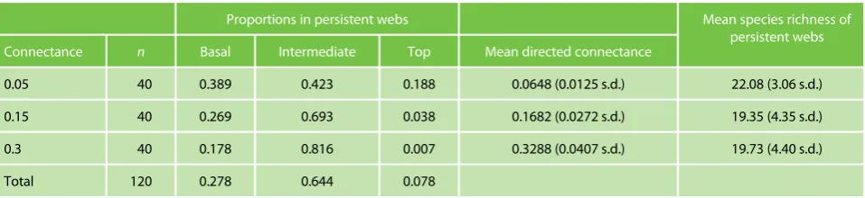
[image:5.612.69.548.587.697.2]The proportions of different trophic groups in persistent webs, as summarized in Table 1, show that as expected connectance increases the prevalence of intermediate species within the communities also increases. The increase
Table 1.The trophic composition, directed connectance and species richness of persistent webs att=2000,nis the number of food webs generated at each level
Proportions in persistent webs Mean species richness of
persistent webs Connectance n Basal Intermediate Top Mean directed connectance
0.05 40 0.389 0.423 0.188 0.0648 (0.0125 s.d.) 22.08 (3.06 s.d.)
0.15 40 0.269 0.693 0.038 0.1682 (0.0272 s.d.) 19.35 (4.35 s.d.)
0.3 40 0.178 0.816 0.007 0.3288 (0.0407 s.d.) 19.73 (4.40 s.d.)
Total 120 0.278 0.644 0.078
. . . .
Research Article Bioscience Horizons•Volume 9 2016
. . . .
in intermediate species prevalence at higher levels of connectance reduces the prevalence of basal and top species to the point that mostC=0.3 webs contain no top species.
The directed connectance of the food webs generated was expected to vary from expected connectance due to the ran-dom community assembly processes, and because webs with a lower connectance are more likely to contain species or loops that match the criteria for web rejection. The values of directed connectance (Table 1) show that all groupings of expected connectance are distinct, despite C = 0.05 webs varying from their actual directed connectance by more than one standard error. The average biomass of species in persist-ent webs was 0.0585.
Successful reintroduction of the subject
species
Thefinal number of simulations included in the analysis for each level of connectance was 599, 600, and 597 simulations atC=0.05, 0.15, and 0.3, respectively, with each of the three times to reintroduction being represented by around 200 simulations. The proportion of subject species of each trophic group is reported in Table2. Full details can be found in the supplementary information.
The initial aim of this work was to determine what factors affect extinction and reintroduction subject species success-fully re-establishing in their communities, indicated by pres-ence of the subject species in thefinal community. In all but 12 cases, the subject species successfully reintroduced accord-ing to this measure.
The 12 simulations where reintroduction species failed to re-establish concerned only four subject species, each of which failed to reintroduce at all durations of time to reintro-duction. Three of the subjects were part of webs where
C = 0.15, and one where C = 0.3. All were intermediate species.
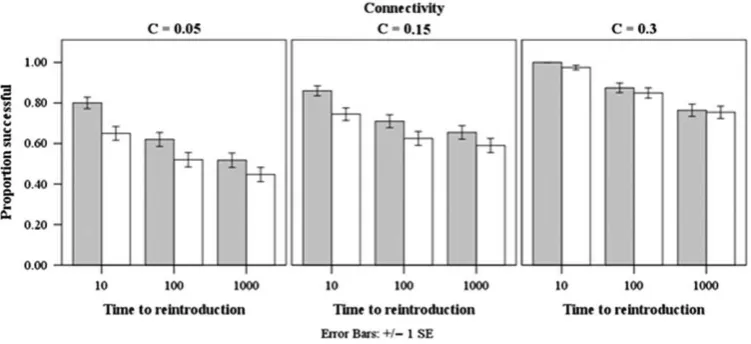
Other measures of reintroduction success
A positive relationship between connectance and reintroduction success can be observed, both when success is measured using species richness and equilibrium biomass change. There is also a negative relationship observable between time to reintroduc-tion and reintroducreintroduc-tion success using these two measured of success. This relationship remains when the three levels of expected connectance are considered separately (Fig.1). [image:6.612.67.299.277.460.2]The trophic group of the reintroduced species can also affect reintroduction success. When success is measured by Table 2.The relative frequency of subject species trophic grouping
Connectance Trophic group Simulations
0.05 Basal 333
Intermediate 176
Top 90
0.15 Basal 219
Intermediate 348
Top 33
0.3 Basal 180
Intermediate 408
Top 9
[image:6.612.119.495.477.649.2]species richness, basal and top species reintroductions gener-ally have lower rates of success than intermediate species reintroduction, in that basal species have a lower success rate than intermediate species by one standard error atC=0.05. This grows to a two standard error difference atC=0.15 and
C=0.03. Although top and intermediate success is indistin-guishable atC=0.05, intermediate species are more success-ful atC=0.15 andC=0.3 by one standard error (Fig.2).
When success is measured by a change in the web’s equilib-rium biomass, intermediate species have generally higher rates of success compared to top species (they differ by one stand-ard deviation at C = 0.05 and 0.15, and by two standard deviations atC=0.03). When compared to basal species this difference is similar, corresponding to one and two standard deviations atC=0.15 and 0.3, respectively. Basal and top species are only meaningfully different atC=0.3 where basal species are more successful by a difference of over two stand-ard deviations (Fig.2).
In no simulation was a basal species present in the com-munity att=2000 lost in thefinal community. This is likely to be due to the simplicity of the model and its underlying deterministic population dynamics. The only way basal spe-cies could go extinct in this model is extreme over-predation or manual removal, and so the removal of predator species will never cause extinction. No convincing relationship could be found between trophic group of the reintroduction subject and the proportion of species lost belonging to each trophic group (Fig.2), aside from the lack of basal species loss.
When basal species are the subject of reintroductions, the mean species loss, of 0.607 (0.0463 s.e.m.), is higher than when the subject species is either an intermediate species, with a mean species loss of 0.207 (0.0202 s.e.m.) or top species, with a mean species loss of 0.993 (0.1772 s.e.m.). This is true at all levels of expected connectance. The relationship
between intermediate and top species at different levels of expected connectance is variable.
Simulations carried out with lower reintroduction bio-masses of 0.1 and 0.0001 (each consisting of 596 simula-tions), at time to reintroduction of 1000, did not vary meaningfully from the results reported for higher reintroduc-tion biomasses.
Species reintroduced in this model have been limited to a reintroduction biomass drawn from a uniform random distri-bution from 0.5 to 1. To test whether this influenced the results, the 598 reintroductions for t = 1000 were re-simulated at low reintroduction biomass (B = 0.1 and
B = 0.0001) and produced only superficial differences at every level of reintroduction success. No additional species failed to reintroduce. Given the mean biomass of persistent communities (B=0.0585), a reintroduction biomass of 0.1 bridges the gap between the mean biomass of persistent com-munities and the reintroduction biomass of 0.5, which we have used to keep our work in line with Romanuk et al.
(2009). The reintroduction biomass of 0.0001 is a relatively low biomass compared to the mean biomass of persistent communities and addresses concerns that our simulations fail to simulate real reintroductions at low biomasses. These results strongly suggest that in these deterministic models of species reintroduction, reintroduction biomass has a minimal effect in shaping thefinal community composition and equi-librium biomass and Romanuket al.’s choice of reintroducing species with a biomass between 0.5 and 1 was justified.
Discussion
[image:7.612.118.495.499.657.2]As anticipated, the longer a species was removed from an eco-logical community, the lower the probability that it could be successfully reintroduced without impacting the wider community. We found a positive relationship between
Figure 2. Reintroduction is more likely to be successful when the subject is a trophically intermediate species. Figure shows the proportion of successful reintroductions for each subject trophic group and connectance combination. Grey bars measure success in terms of secondary extinctions, white bars in terms of change to equilibrium biomasses. Error bars are±1 standard error of the mean.
. . . .
Research Article Bioscience Horizons•Volume 9 2016
. . . .
connectance and proportion of successful reintroductions, as measured by species richness and biomass equilibrium. More connected webs also lost fewer species on average. Thesefi nd-ings agree with other theoretical work suggesting that more connected webs are more robust to species removal
(Camacho, Guimera and Amaral, 2002;Dunne, Williams and
Martinez, 2002).
Although these results fail to show a relationship between the time to reintroduction and reintroduction species success, the study identifies important relationships between community-level measures of success and time to reintroduc-tion, web connectance, and trophic grouping of the reintro-duced species.
If the subject of an extinction and reintroduction is a basal or top species, the probability that the community will recover to the same species richness or biomass equilibrium is lower than if the subject species is an intermediate species. This is consistent across all levels of connectance examined in this study. Intermediate reintroduction subject simulations have the lowest values of species loss at all levels of expected con-nectance. It is notable that these results corroborate thefi nd-ings of some extinction models (Borrvall, Ebenman and Jonsson, 2000;Eklof and Ebenman, 2006) and is consistent with arguments both for a bottom up and top-down deter-mination of species richness.
Apart from the lack of any basal species loss during the simulations, there is no evidence to suggest that the species lost from communities are selected non-randomly from top and intermediate species groups. However, due to the prevalence of intermediate species in the food webs (Table1), especially at higher values of connectance, it would be difficult to detect non-random loss of intermediate and top species. Studies sug-gest a higher number of top species should have become extinct due to top predator vulnerability (Sanders, Sutter and van Veen, 2013). In our simulations the predators in general were more vulnerable, and no basal species went extinct.
Species richness of persistent communities att=2000 was lower inC=0.3 andC=0.15 than inC=0.05 (Table1); however, there was overlap within one standard deviation. This suggests that connectance does not affect persistent com-munity species richness and is consistent with some studies of connectance and species richness (Fox and McGrady-Steed, 2002). However, it does notfit with the hyperbolic connec-tance relationship (Chen and Cohen, 2000), or inverse rela-tionship suggested in other work (Keitt, 1997; Laird and Jensen, 2007).
For models to be useful, they must be presented simply and clearly. The results of both Romanuk et al. (2009) and
Williams and Martinez (2000)are difficult to replicate with-out ambiguity. For example, it is unclear whether top species include cannibalistic species, or only species that have no pre-dators. These two definitions are not identical, and in our simulations they lead to slightly different success results. Similarly, it is not clear whether Romanuk et al. (2009)
removed trophically identical or disconnected species as in
Williams and Martinez (2000). The MATLAB scripts for our
simulations are included in the supplementary information for the sake of transparency.
Although modifications to the niche model have been sug-gested (Allesina, Alonso and Pascual, 2008; Cattin et al., 2004),Romanuk et al. (2009)argued that their original mod-el maintained the most accurate fit to empirical data (Williams and Martinez, 2008). However, the model is unable to simulate webs with a connectance equal to or greater than 0.5 and can have difficulty simulating webs with connectance approaching 0.5. Moreover, it tends to create food webs with less variability and more intervality than those found in empirical systems (Romanuket al., 2009). The variableriin
the niche model is also drawn from a restrictedβdistribution whereα=1.Williams and Martinez (2000)state that this is to ease calculation difficulty. The consequences of allowingα
andβto vary (so long as the expected value of 2Cis main-tained) are currently unstudied.
The food webs are constructed and simulated with regard to the feeding relationships of species. The models do not incorporate other ecological interactions that may not be dir-ectional, such as mutualisms that benefit both species. The term ‘extinction’ has been used throughout this work. However, given that the species is later reintroduced, at worst this‘extinction’refers either to the extinction of a species in the wild, or to a local extinction. Extinction, in the sense of this work, is a state where the species in question is no longer interacting trophically with the other species in its native com-munity. Equally, reintroduction refers only to the return of that species to its native community. The population dynam-ics observed in this work typically occur at time scales on of the order of 10 time steps. Therefore, in regard to the dynam-ics of the system, the three times to reintroduction can be thought of as:
t=10: the system has very been recently affected by the removal of a single species, but many subsequent effects of this extinction (e.g. secondary extinctions) have yet to occur.
t=100: the system is beginning to equilibrate, and second-ary extinctions may have occurred, but the community is still changing and has not reached an equilibrium. Species loss can still be prevented by reintroduction in principle, but much of the damage is already done.
t=1000: the system has now reached, or is very close to, a new equilibrium point.
In the broadest terms, in a terrestrial community operating at annual time scales it would be appropriate to think of
T=10, 100 and 1000 corresponding to reintroductions after times of 1, 10 and 100 years, respectively.
in that it ignores possible stress, low genetic diversity among other factors. Despite this, the fact that consistent and practic-ally interpretable trends emerge from the simulations ought to provide useful general insight.
The simulations presented here assume that, given a food web and a set of parameters, the community dynamics are deterministic. Factors such as environmental and demo-graphic stochasticity, and non-random drivers such as evolu-tion, mean that real communities may be in a constant state of disequilibrium. It may be argued that over short time scales, and for large populations, a deterministic mean-field dynamics may operate, but this ought not to be regarded as self-evident (Van Kampen, 2007).
Author
’
s biography
Justin Byrne is a Masters student at the University of York, currently researching avian communities in the Albertine Rift. Previously he studied Biology (with a year in industry) at the University of York. He spent a year in industry at Kew’s Millenium seed bank and then conducted this work as a dis-sertation project. He designed research, conducted research, analysed data, and wrote the paper. He has primary responsi-bility for thefinal content. Jon Pitchford is a Reader in math-ematical ecology at the University of York. Jon designed research, and contributed to the analysis, writing, and revi-sion of this work where specialist knowledge of mathematics was required.
Funding
No funding was received for this work.
References
Allesina, S., Alonso, D. and Pascual, M. (2008) A general model for food web structure,Science, 320 (5876), 658–661.
Armstrong, D. P. and Ewen, J. G. (2002) Dynamics and viability of a New Zealand robin population reintroduced to regenerating fragmen-ted habitat,Conservation Biology, 16 (4), 1074–1085.
Armstrong, D. P. and Seddon, P. J. (2008) Directions in reintroduction biology,Trends in Ecology & Evolution, 23 (1), 20–25.
Bennett, V. A., Doerr, V. A. J., Doerr, E. D. et al. (2013) Causes of reintro-duction failure of the brown treecreeper: Implications for ecosys-tem restoration,Austral Ecology, 38 (6), 700–712.
Borrvall, C., Ebenman, B. and Jonsson, T. (2000) Biodiversity lessens the risk of cascading extinction in model food webs,Ecology Letters, 3 (2), 131–136.
Brose, U., Berlow, E. L. and Martinez, N. D. (2005) Scaling up keystone effects from simple to complex ecological networks,Ecology Letters, 8 (12), 1317–1325.
Brose, U., Williams, R. J. and Martinez, N. D. (2006) Allometric scaling enhances stability in complex food webs,Ecology Letters, 9 (11), 1228–1236.
Camacho, J., Guimera, R. and Amaral, L. A. N. (2002) Robust patterns in food web structure,Physical Review Letters, 88 (22), 4.
Cardinale, B. J., Duffy, J. E., Gonzalez, A. et al. (2012) Biodiversity loss and its impact on humanity,Nature, 486 (7401), 59–67.
Cattin, M. F., Bersier, L. F., Banasek-Richter, C. et al. (2004) Phylogenetic constraints and adaptation explain food-web structure,Nature, 427 (6977), 835–839.
Courchamp, F., Berec, L. and Gascoigne, J. (2008)Allee Effects in Ecology and Conservation, Oxford University Press, Oxford, UK.
Chen, X. and Cohen, J. E. (2000) Support of the hyperbolic connectance hypothesis by qualitative stability of model food webs,Community Ecology, 1 (2), 215–225.
Cohen, J. E., Briand, F. and Newman, C. M. (1990)Community Food Webs: Data and Theory, Springer, Berlin, Germany.
Davidson, R. S. and Armstrong, D. P. (2002) Estimating impacts of poi-son operations on non-target species using mark-recapture analysis and simulation modelling: an example with saddlebacks,Biological Conservation, 105 (3), 375–381.
Dunne, J. A., Williams, R. J. and Martinez, N. D. (2002) Network structure and biodiversity loss in food webs: robustness increases with con-nectance,Ecology Letters, 5 (4), 558–567.
Eklof, A. and Ebenman, B. (2006) Species loss and secondary extinctions in simple and complex model communities, Journal of Animal Ecology, 75 (1), 239–246.
Fox, J. W. and McGrady-Steed, J. (2002) Stability and complexity in microcosm communities,Journal of Animal Ecology, 71 (5), 749–756. Godefroid, S., Piazza, C., Rossi, G. et al. (2011) How successful are plant
species reintroductions?Biological Conservation, 144 (2), 672–682. Holling, C. S. (1959a) Some characteristics of simple types of predation
and parasitism,The Canadian Entomologist, 91 (7), 385–398. Holling, C. S. (1959b) The components of predation as revealed by a
study of small-mammal predation of the European Pine Sawfly,The Canadian Entomologist, 91 (5), 293–320.
IUCN/SSC (2013)Guidelines for Reintroductions and Other Conservation Translocations. Version 1.0, Gland, Switzerland: IUCN Species Survival Commission, viiii+57 pp.
James, A., Pitchford, J. W. and Plank, M. J. (2012) Disentangling nested-ness from models of ecological complexity, Nature, 487 (7406), 227–230.
James, A., Pitchford, J. W. and Plank, M. J. (2013) Jameset al. reply,
Nature, 500 (7463), E2–E3.
Jule, K. R., Leaver, L. A. and Lea, S. E. G. (2008) The effects of captive experience on reintroduction survival in carnivores: a review and analysis,Biological Conservation, 141 (2), 355–363.
. . . .
Research Article Bioscience Horizons•Volume 9 2016
. . . .
Keitt, T. H. (1997) Stability and complexity on a lattice: coexistence of species in an individual-based food web model, Ecological Modelling, 102 (2–3), 243–258.
Laird, S. and Jensen, H. J. (2007) Correlation, selection and the evolu-tion of species networks,Ecological Modelling, 209 (2–4), 149–156. Martinez, N. D. (1991) Artifacts or attributes–effects of resolution on
the little-rock lake food web, Ecological Monographs, 61 (4), 367–392.
Martinez, N. D., Williams, R. J. and Dunne, J. A. (2006) Diversity, com-plexity, and persistence in large model ecosystems, in M.Pascual and J. A.Dunne (eds), Ecological Networks: Linking Structure to Dynamics in Food Webs, Oxford University Press, Oxford, UK, pp. 167–185.
May, R. M. (1972) Will a large complex system be stable,Nature, 238 (5364), 413–414.
McCann, K. and Hastings, A. (1997) Re-evaluating the omnivory-stability relationship in food webs,Proceedings of the Royal Society B–Biological Sciences, 264 (1385), 1249–1254.
McCann, K., Hastings, A. and Huxel, G. R. (1998) Weak trophic interac-tions and the balance of nature,Nature, 395 (6704), 794–798.
McCann, K. and Yodzis, P. (1995) Bifurcation structure of a 3-species food-chain model, Theoretical Population Biology, 48 (2), 93–125.
Nolet, B. A. and Baveco, J. M. (1996) Development and viability of a translocated beaver Castor fiber population in the Netherlands,
Biological Conservation, 75 (2), 125–137.
Proulx, S. R., Promislow, D. E. L. and Phillips, P. C. (2005) Network think-ing in ecology and evolution,Trends in Ecology & Evolution, 20 (6), 345–353.
Ren, H., Jian, S. G., Liu, H. X. et al. (2014) Advances in the reintroduction of rare and endangered wild plant species, Science China-Life Sciences, 57 (6), 603–609.
Ripple, W. J. and Beschta, R. L. (2012) Trophic cascades in Yellowstone: thefirst 15 years after wolf reintroduction,Biological Conservation, 145 (1), 205–213.
Romanuk, T. N., Zhou, Y., Brose, U. et al. (2009) Predicting invasion suc-cess in complex ecological networks,Philosophical Transactions of the Royal Society B–Biological Sciences, 364 (1524), 1743–1754. Sanders, D., Sutter, L. and van Veen, F. J. F. (2013) The loss of indirect
interactions leads to cascading extinctions of carnivores, Ecology Letters, 16 (5), 664–669.
Seddon, P. J., Armstrong, D. P. and Maloney, R. F. (2007) Developing the sci-ence of reintroduction biology,Conservation Biology, 21 (2), 303–312.
Van Kampen, N. G. (2007)Stochastic Processes in Physics and Chemistry, Elsevier, Amsterdam.
Williams, B. K. (1997) Logic and science in wildlife biology,Journal of Wildlife Management, 61 (4), 1007–1015.
Williams, R. J. and Martinez, N. D. (2000) Simple rules yield complex food webs,Nature, 404 (6774), 180–183.
Williams, R. J. and Martinez, N. D. (2004) Stabilization of chaotic and non-permanent food-web dynamics, European Physical Journal B, 38 (2), 297–303.
Williams, R. J. and Martinez, N. D. (2008) Success and its limits among structural models of complex food webs,Journal of Animal Ecology, 77 (3), 512–519.