A fuzzy mixed integer linear programming model for integrating procurement-production-distribution planning in supply chain Pages 403-412 Download PDF

* Corresponding author. Tel.: +989368928114 E-mail: [email protected] (A. Pouroosta) © 2012 Growing Science Ltd. All rights reserved. doi: 10.5267/j.ijiec.2011.12.006

   

Contents lists available at GrowingScience

International Journal of Industrial Engineering Computations

homepage: www.GrowingScience.com/ijiec

A fuzzy mixed integer linear programming model for integrating procurement-production-distribution planning in supply chain

 

Alireza Pourroustaa*, Saleh Dehbaria, Reza Tavakkoli-Moghaddamb, Amir Imenpourcand Mahdi Naderi-Benia

a

Department of Industrial Engineering, Islamic Azad University, South Tehran Branch,Tehran, Iran

b

Department of Industrial Engineering, Colleague of Engineering, University of Tehran, Tehran, Iran

c

Department Graduate School of Management and Economic, Sharif University of Technology, Tehran, Iran

A R T I C L E I N F O A B S T R A C T

Article history:

Received 15 October 2011 Received in revised form November, 26, 2011 Accepted 26 December 2011 Available online

14 December 2011

In this paper, we study a supply chain problem where a whole seller/producer distributes goods among different retailers. Such problems are always faces with uncertainty with input data and we have to use various techniques to handle the uncertainty. The proposed model of this paper considers different input parameters such as demand, capacity and cost in trapezoid fuzzy forms and using two ranking methods, we handle the uncertainty. The results of the proposed model of this paper have been compared with the crisp and other existing fuzzy techniques using some randomly generated data. The preliminary results indicate that the proposed models of this paper provides better values for the objective function and do not increase the complexity of the resulted problem.

© 2012 Growing Science Ltd. All rights reserved

Keywords:

Jimenez fuzzy technique Cadenas & Verdegay fuzzy technique

VRP Time window

1. Introduction

404

Jayaraman and Ross (2003) investigated a system of distribution network design problems characterized by multiple product families, a central manufacturing plant site, multiple distribution center and cross-docking sites, and retail outlets (customer zones) which demand multiple units of various commodities. Syarif et al. (2002) presented a logistic chain network problem, which is a 0–1 mixed integer linear programming model. The design tasks of this problem presented the choice of the facilities to be opened and the distribution network design to satisfy the demand with minimum cost. They used the spanning tree-based genetic algorithm by implementing Prüfer number representation. The efficiency of the proposed method was examined by comparing its numerical experiment results with those of conventional matrix-based genetic algorithm. Zhou et al. (2002) implemented a genetic algorithm for a balanced allocation of customers to multiple distribution centers in the supply chain network. Petrovic et al. (1999) presented some solution procedures for solving supply chain problem using the concept of fuzzy programming.

Liang (2008) presented a fuzzy objective production/distribution planning decisions with multi-product and multi-time period in a supply chain. Liang extended a fuzzy multi-objective linear programming (FMOLP) system with piecewise linear membership function to handle integrated multi-product and multi-time period production/distribution planning decisions (PDPD) problems where the objectives are formulated in fuzzy form.

The work extends the original multi-objective linear programming to minimize total costs and total delivery time associated with inventory levels, available machine capacity and labor levels at each source, and predicts demand and available warehouse space at each destination and total budget. The proposed FMOLP model presents a systematic framework, which facilitates fuzzy decision-making process to adjust the search direction during the solution procedure to obtain a DM’s efficient solution. In addition, the DM calculates the value in each cost category by studying the time value of money in the proposed model.

Dubois et al. (2003) studied different fuzzy set-based approaches for scheduling which includes representing preference profiles and modeling uncertainty distributions. Chen and Chang (2006) presented a mathematical programming method for supply chain models with fuzzy parameters. Liang (2008) presented an integrated production-transportation planning decision with fuzzy multiple objectives in supply chains. Aliev et al. (2007) used fuzzy-genetic approach to aggregate production-distribution planning in supply chain management.

Dehbari et al. (2012) presented a supply chain problem where a whole seller/producer distributes goods among various retailers. The model was formulated as a more general and realistic form of traditional vehicle routing problem (VRP). The problem was solved using a hybrid of particle swarm optimization and simulated annealing (PSO-SA) and the results were compared with other hybrid method, which was a hybrid of Ant colony and Tabu search. They implemented some well-known benchmark problems to compare the results of the proposed model with other method.

Liang and Cheng (2009) applied fuzzy sets for an integrated manufacturing/distribution planning decision (MDPD) problems with multi-product and multi-time period in supply chains. The proposed model considered time value of money for each of the operating cost categories and using fuzzy multi-objective linear programming model (FMOLP) minimizes total costs and total delivery time with reference to inventory levels, available machine capacity and other issues, simultaneously. They used an industrial case to demonstrate the feasibility of the proposed model for a realistic MDPD problem.

In this paper, we present an integrated supply chain by considering different parameters with uncertainty using trapezoid numbers. The proposed model of this paper is solved using two different fuzzy programming techniques. The organization of this paper first presents the necessary notations and problem formulations in section 2 and some numerical solution is given in section 3, finally, the paper concludes the results and suggests some future works.

2. Problem statement

2.1. Problem definition

The proposed model of this paper consists of four different stages. In the first stage, the SC considers suppliers providing raw material and work in process for different factories. The second stage considers factories, which produce the final product. In the third stage, the network includes distribution centers, which are responsible for shipping final products to different locations. Finally, the last stage includes sales zones. The following assumptions hold for the proposed model of this paper,

• The supply chain includes suppliers, factories, distributers and sales centers,

• There are four cost items including purchasing, production, transportation, setup and holding, • The input data are inventory capacity, production capacity, consumption rate, demand and

supply,

• The outputs are appropriate program for purchasing, production of each factory in each period, optimal inventory level in factories and distribution centers, the amount of raw material shipped from supplier to factory and from factory to distribution center and from distribution center to end customer via sales' centers.

We consider a medium term planning and all parameters are in trapezoid fuzzy numbers. Table 1 shows the necessary parameters and decision variables,

Table 1

Necessary notations and decision variables Set of indices

S set of suppliers ( 1,2, … , ) P set of plants ( 1,2, … , )

406

Parameters

j_rst

SC fuzzy purchasing cost of raw material r from supplier s at period t

j

gpt

PC fuzzy variable production cost of finished product g in plant p at period t Fgpt fixed production cost of finished product g in plant p at period t

HRrpt holding cost of raw material r in plant p at period t HGgpt holding cost of finished product g in plant p at period t

HWgwt holding cost of finished product g in distribution center w at period t TRrspt transportation cost of raw material r from supplier s to plant p at period t TGgpwt transportation cost of finished product g from plant p to DC w at period t TWgwzt transportation cost of finished product g from DC w to CZ z at period t

i_gzt

D fuzzy demand of finished product g at CZ z at period t

k

gpt

cap fuzzy production capacity of plant p for finished product g at period t

βrst maximum supply raw material r by supplier s at period t

i

gwt

V fuzzy maximum holding capacity for finished product g in DC w at period t

αrg quantity of raw material r consumed in finished product g

 

Decision variables:

qrst quantity of raw material r supplied from supplier s at period t

xrspt quantity of raw material r shipped from supplier s to plant p at period t RIrpt inventory level of raw material rin plant pat period t

ygpt quantity of finished product g produced in plant p at period t GIgpt inventory level of finished product g in plant p at period t WIgwt inventory level of finished product g in DC w at period t

mgpwt quantity of finished product g shipped form plant p to DC w at period t ngwzt quantity of finished product g shipped form DC w to CZ z at period t

1 0 gpt

k = ⎨⎧

⎩  

if finished product g produced in plant p at period t Otherwise

2.2 Problems formulation

The first objective function of the proposed model given in Eq. (1) minimizes total cost of purchasing items, setup of each product in each factory, production, inventory cost items including the cost of raw material, final product in factory and distribution centers. The objective function of the proposed model also minimizes transportation cost of raw material, final product in factory and distribution centers.

) 1 (

j

(

j

)

min rst _{rst gpt gpt} gpt _{gpt gpt rspt}

r s p t

r s t g p t

gpwt gpwt gwzt gwzt rpt rpt gwt gwt

t

gp

t t t

g p w g w z r p g

t

w

rspt

Z SC q F z PC y HG GI TR

TG m TW n HR RI

x

HW WI

= + + + +

+ + + +

∑∑∑∑

∑∑∑

∑∑∑

∑

∑

∑

∑

∑∑∑

∑∑∑

∑∑

∑∑

subject to

) 2 ( , ,

r s t

∀

rst rspt

p

q ≥

∑

x

) 3 ( , ,

r p t

∀

, 1 .

rpt rp t rspt rg gpt

s g

RI =RI − +

∑

x −

∑

α

y

) 4 ( , ,

g p t

∀

, 1

gpt gp t gpt gpwt

w

) 5 ( , ,

g w t

∀ , 1

gwt gw t gpwt gwzt

p z

W I =WI − +

∑

m −

∑

n

) 6 ( , ,

g z t

∀

i_gzt

gw zt w

n

D ≤

∑

) 7 ( , ,

g p t

∀

k

gpt gpt gpt

y ≤cap k

) 8 ( , ,

g w t

∀

i_gwt

gpwt p

m ≤V

∑

) 9 ( , ,

r s t

∀

rst rst

q ≤

β

 

) 10 ( , ,

g p t

∀

.

gpwt gpt

w

m ≤M k

∑

 

) 11 ( , , , , , ,

r s p t g w z

∀

, , , , , , , , 0, {0,1}

rst rspt rpt gpt gpt gwt gpwt gwzt gwt gpt

q x RI y GI W I m n B ≥ k ∈  

Constraints (2) ensures that the amount of supplied raw material is, at least, equal to the amount of raw material shipped to all factories. Eq. (3) shows that the amount of raw material in each period is equal to the amount of inventory in the previous period and the amount of raw material shipped to factory in this period minus the consumption in this period. Eq. (4) and Eq. (5) do similarly for production and distribution centers. Eq. (6) determines the maximum demand for each distribution center. Eq. (7) and Eq. (8) show the maximum production capacity of each production and distribution centers, respectively. Eq. (9) determines the maximum supply and Eq. (10) ensures that when product is about to be delivered, the production must be setup and accomplished. Finally, Eq. (11) ensures the non-negativity of variables.

2.3. Fuzzy model one (Jimenez's model)

In this section, we present a fuzzy approach to handle the uncertainty and implement the ranking method introduced by Jimenez et al. (2007) to defuzzify the fuzzy numbers. Consider a trapezoid fuzzy number Ai=

{

a a a a₁, , ,_{2 3 4}

}

as follows,

) 12 (

i

( )

( )

1 1 2 2 3 3 4 4

0 ; ( , ]

( ) ; [ , ]

1 ; [ , ]

; [ , ]

0 ; [ , )

A

A

A

x a

f x x a a

x x a a

g x x a a

x a μ ⎧ _{∀ ∈ − ∞} ⎪ ∀ ∈ ⎪ ⎪ = ⎨ ∀ ∈ ⎪ ∀ ∈ ⎪ ⎪ _{∀ ∈ ∞} ⎩

In order to make sure that 1_{( )} A

f − x and g_A−1

( )

x we assume that f_A( )x is a continuous and non-decreasing function and g_A

( )

x is a continuous and non-increasing function. Therefore, we have

Using some simplification yields the following,

i

( )

i i

( )

( )

1 1

1 1

1 2

0 0

, A , A .

A A

EI A E E f−

α α

d g−

α α

d

⎡ ⎤ ⎡ ⎤ =_⎣ =⎢ − ⎥ ⎦ ⎢_⎣

∫

∫

⎥_⎦

) 14 ( ) 13 ( i

( )

i i 2 4

1 3

1, 2 ( ), ( ) .

a a

A A

a a

A A

EI A E E xdf x xdg x

⎡ ⎤

⎡ ⎤ ⎢ ⎥

=_⎣ = −

408

When ( )f_A x and g_A

( )

x are linear we can simply the equations as follows,

i

( )

1 2 3 4

1_{( ), (}1 ₎

2 2

EI A =⎡_⎢ a +a a +a ⎤_⎥

⎣ ⎦

(15)

In addition, to compare two fuzzy numbers we use the following,

i i

( )

₍

₎

2 1

2 1

1 2 2 1

2 2 1 2

1 2

0 if 0

, if 0 ,

1 if 0

a b

A B

a b a b

M A B A B

a b

E E

E E

A B E E E E

E E E E

E E

μ

⎧ _{− <}

⎪

⎪ − _{⎡ ⎤}

=_⎨ = ∈_⎣ − − _⎦

− − −

⎪

⎪ _{− >}

⎩

, (16)

where , and , are expected values of and , respectively. For more details the interested readers are suggested to read Jimenez et al. (2007).

The mathematical model given in Eq. (1) to Eq. (1 1 in fuzzy form is as follows, )

) 17 (

(

1 2 3 4

)

1 2 3 4

1 min 4 1 ( ) 4

rst rst rst rst rst

r s t

gpt gpt gpt gpt gpt gpt gpt gpt gpt

g p t

rspt rspt gpwt gpwt gwzt gwzt

r s p t g p w t g w z t

Z SC SC SC SC q

F z PC PC PC PC y HG GI

TR x TG m TW n

= + + + ⎛ ⎞ + _⎜ + + + _⎟ ⎝ ⎠ + + + + +

∑∑∑

∑∑∑

∑∑∑∑

∑∑∑∑

∑∑∑∑

_{rpt rpt gwt gwt}

r p t g w t

HR RI HW WI

+

∑∑∑

+

∑∑∑

) 18 ( , ,

g z t

∀ subject to

(

1

)

1 2 3 4

2 2

gzt gzt gzt gzt

gwzt w

D D D D

n α + α + − + ≤

∑

) 19 ( , ,

g p t

∀

(

)

3 4 1 2

1

2 2

gwt gwt gwt gwt

gpt gpt

cap cap cap cap

y ≤⎛⎜_⎜ −α + +α + ⎞⎟_⎟k

⎝ ⎠

) 20 ( , ,

g w t

∀

(

1

)

3 4 1 2

2 2

gwt gwt gwt gwt

gpwt p

V V V V

m ≤ −

α

+ +

α

+

∑

The other equations are the same as the crisp model.

2.4. Fuzzy model two (Cadenas and Verdegay model)

1 max n _{j j}

j

Z c x

=

=

∑

1 n

ij _{j f} i

j

a x b

=

≤

∑

0, , xj ≥ i∈M j∈N

(21)

where the cost is defined as follows,

( )

μ_j F

∃ ∈ R such thatμ_j:R→[0,1] j∈N. (22)

The right hand sides are also defined as follows,

such that μ_i :R→[0,1]i∈M

( )

μi F

∃ ∈ R (23)

In addition, for each constraint, we have,

( )

μi F(F

∃ ∈ R such that i∈M μi : F

( )

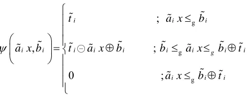
R →[0,1] (24)

One general approach to solve the fuzzy linear programming given by Eq. (25) is to use convex fuzzy sets as follows,

g g

g ;

, ;

0 ;

i i

i i i i i i i

i

i i

g

i i i

t a x b

a x b t a x b b a x b t

a x b t

ψ

⎧

≤ ⎪

⎪

⎛ ⎞ ⎪_{= ⊕ ≤ ≤ ⊕}

⎨

⎜ ⎟

⎝ ⎠ ⎪

⎪ _{≤ ⊕}

⎪⎩

(25)

and the fuzzy linear programming model is summarized in the following form,

1 max n j _j

j c x =

∑

subject to

(

)

i g 1

1 α

n

ij _j i

j

a x b t i M

=

≤ + − ∈

∑

(26)

0, [0,1], j

x ≥ α∈ j∈N

For more details, please see Cadenas and Verdegay (1997).

3. Numerical solution

In this section we present some results for the implementation of the proposed fuzzy models and compare our results with crisp model. The fuzzy parameters of the proposed models are uniformly distributed and they are given in Table 2.

Table 2

Input parameters Parameter

410

In this model, demand is given in fuzzy form as 60,80,100,120 , the capacity for each product in each period is 670, the production capacity of each factory is 340,360,400,420 and finally the capacity of each distribution center is 390,400,490,520. We consider quarterly or semi-annual planning horizon. The resulted problem formulations for two fuzzy models as well as crisp one have been solved using Lingo software and the results are summarized in Table 3.

Table 3

The results of the implementation of the propose fuzzy models

Jimenez Method

Problem |S| |P| |W| |Z| Crisp Cadenas α=0.2 α=0.7 α=1 1 3 2 2 2 32862 29769 27384 32877 36183

2 3 2 4 6 97319 85832 78214 94741 105104 3 5 3 4 6 87986 78002 71403 86111 95640

4 5 3 6 8 120133 106650 97412 119328 132873 5 10 4 6 8 170465 150841 135045 167438 188462

6 10 4 8 10 215570 189711 170724 209545 233224 7 20 5 8 10 206619 181920 164160 200717 222616

8 20 5 10 12 247551 219320 200125 244866 272545

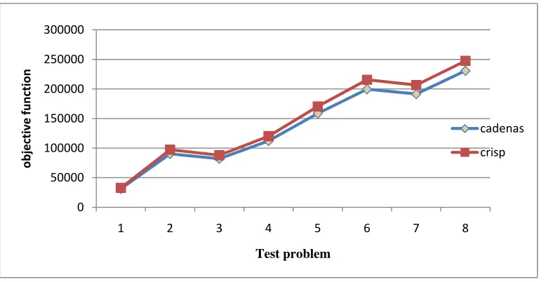
As we can observe from the results of Table 3, both fuzzy models provide better objective values compared with the crisp model and Fig. 1 demonstrates the results of the implementation of the first fuzzy model versus crisp model.

Fig. 1. The performance of cadenzas and crisp model

As we can observe from the results of Fig. 1, when α=0.2the proposed fuzzy model outperforms the crisp model and for other cases, there are not much differences between two methods. In addition, Fig. 2 shows the relative performance of the second fuzzy model versus crisp model.

0 50000 100000 150000 200000 250000 300000

1 2 3 4 5 6 7 8

obj

ect

ive

fu

nc

ti

on

Test problem

jimenez (α=0.2)

jimenez (α=0.7)

jimenez (α=1)

Fig. 2. The performance of the crisp model versus the second fuzzy model

It is clear from the results that the proposed model mostly beats the crisp model.

4. Conclusion

In this paper, we have investigated a supply chain problem where a whole seller/producer distributes goods among different retailers. The resulted problem were often faced with uncertainty and the input data are perturbed with some noises. Therefore, we need to implement various techniques to handle the uncertainty. The proposed model of this paper investigated different input parameters such as demand, capacity and cost in trapezoid fuzzy forms and using two ranking methods, we handled the uncertainty. The results of the proposed model of this paper have been compared with the crisp and other existing fuzzy techniques using some randomly generated data and our comparison indicated that the proposed model of this paper could provide somewhat lower values for the objective function and do not increase the complexity of the resulted problem.

Acknowledgment

The authors would like to thank the anonymous referees for the comments on earlier version of this work, which helped us improve the quality of the paper.

References

Aliev, R.A., Fazlollahi, B., Guirimov, B.G., & Aliev, R.R.(2007). Fuzzy-genetic approach to aggregate production-distribution planning in supply chain management. Information Sciences, 177, 4241-4255.

Bilgen, B. (2010). Application of fuzzy mathematical programming approach to the production allocation and distribution supply chain network problem. Expert system with applications, 37, 4488-4495.

Cadenas, J.M., & Verdegay J.L. (1997). Using fuzzy numbers in linear programming. IEEE Transactions on Systems. Man and Cybernetics Part B-Cybernetics, 27, 1016-1022.

Chen, S.P., & Chang, P.C.(2006). A mathematical programming approach to supply chain models with fuzzy parameters. Engineering Optimization, 38, 647-669.

Davis, T. (1993). Effective supply chain management. Sloan Management Review, 34, 35-46.

Dehbari, S., Pourrousta, A., Ebrahim Neghad, S., Tavakkoli-Moghaddam, R., & Javanshir, H.(2012). A new supply chain management method with one-way time window: A hybrid PSO-SA approach.International Journal of Industrial Engineering Computations,3(2), 241-252.

0 50000 100000 150000 200000 250000 300000

1 2 3 4 5 6 7 8

ob

ject

iv

e

 

function

Test problem

cadenas

412

Dubois, D., Fargier, H., & Fortemps, P. (2003). Fuzzy scheduling: modelling flexible constraints vs. coping with incomplete knowledge. European Journal of Operational Research, 147, 231-252. Jayaraman, V., & Ross, A. (2003). A simulated annealing methodology to distribution network

design and management. European Journal of Operational Research, 144, 629-645.

Jimenez, M., Arenas, M., Bilbao, A., & Guez, M.V. (2007). Linear programming with fuzzy parameters: an interactive method resolution. European Journal of Operational Research, 177, 1599-1609.

Liang, T.F. (2008). Fuzzy objective production/distribution planning decisions with multi-product and multi-time period in a supply chain. Computers & IndustrialEngineering, 55(3), 676-694.

Liang, T.F.(2008). Integrating production-transportation planning decision with fuzzy multiple goals in supply chains. International Journal of Production Research, 46, 1477-1494.

Liang, T.F., Cheng, & H.W. (2009). Application of fuzzy sets to manufacturing/distribution planning decisions with multi-product and multi-time period in supply chains. Expert Systems with Applications, 36, 3367-3377.

McDonald, C.M., & Karimi, I.A.(1997). Planning and scheduling of parallel semi-continuous processes. Industrial & Engineering Chemical Research, 36, 2691-2700.

Mula, J., Peidro, D., & Poler, R. (2010). The effectiveness of a fuzzy mathematical programming approach for supply chain production planning with fuzzy demand. International Journal of Production Economics,128, 136-143.

Peidro, D., Mula, J., Poler, R., & Verdegay, J.L. (2009). Fuzzy optimization for supply chain planning under supply, demand, and process uncertainties. Fuzzy Sets and Systems, 160, 2640-2657.

Peidro, D., Mula, J., Jimenez, M., & Botela, M.D.M. (2010). A fuzzy linear programming based approach for tactical supply chain planning in an uncertainty environment. European Journal of Operational Research, 205, 65-80.

Petrovic, D. Roy, R., & Petrovic, R.(1999). Supply chain modelling using fuzzy sets. International Journal of Production Economics, 59, 443-453.

Simchi-Levi, D., Kaminsky, P., & Simchi-Levi, E. (2000). Designing and Managing the Supply Chain: Concepts, Strategies, and Case Studies. McGraw-Hill, New York.

Sabri, E.H., & Beamon, B.N. (2000). A multi-objective approach to simultaneous strategic and operational planning in supply chain design. Omega, 28, 581-598.

Syarif, N., Yun, Y., & Gen, M. (2002). Study on multi-stage logistic chain network: a spanning tree based genetic algorithm approach. Computers & Industrial Engineering, 43, 299-314.

Torabi, S.A., & Hassini, E. (2008). An interactive possibilistic programming approach for multiple objective supply chain master planning. Fuzzy Sets and Systems, 159, 193-214.