www.the-cryosphere.net/11/407/2017/ doi:10.5194/tc-11-407-2017
© Author(s) 2017. CC Attribution 3.0 License.
Spatial variability in mass loss of glaciers in the Everest region,
central Himalayas, between 2000 and 2015
Owen King1, Duncan J. Quincey1, Jonathan L. Carrivick1, and Ann V. Rowan2
1School of Geography and water@leeds, University of Leeds, Leeds, LS2 9JT, UK 2Department of Geography, University of Sheffield, Sheffield, S10 2TN, UK
Correspondence to:Owen King ([email protected])
Received: 25 April 2016 – Published in The Cryosphere Discuss.: 23 May 2016 Revised: 27 December 2016 – Accepted: 9 January 2017 – Published: 3 February 2017
Abstract.Region-wide averaging of Himalayan glacier mass change has masked any catchment or glacier-scale variabil-ity in glacier recession; thus the role of a number of glacio-logical processes in glacier wastage remains poorly under-stood. In this study, we quantify mass loss rates over the period 2000–2015 for 32 glaciers across the Everest region and assess how future ice loss is likely to differ depend-ing on glacier hypsometry. The mean mass balance of all 32 glaciers in our sample was−0.52±0.22 m water equiva-lent (w.e.) a−1. The mean mass balance of nine lacustrine-terminating glaciers (−0.70±0.26 m w.e. a−1) was 32 % more negative than land-terminating, debris-covered glaciers (−0.53±0.21 m w.e. a−1). The mass balance of
lacustrine-terminating glaciers is highly variable (−0.45±0.13 to
−0.91±0.22 m w.e. a−1), perhaps reflecting glacial lakes at different stages of development. To assess the importance of hypsometry on glacier response to future temperature in-creases, we calculated current (Dudh Koshi – 0.41, Tama Koshi – 0.43, Pumqu – 0.37) and prospective future glacier accumulation area Ratios (AARs). IPCC AR5 RCP 4.5 warming (0.9–2.3◦C by 2100) could reduce AARs to 0.29 or 0.08 in the Tama Koshi catchment, 0.27 or 0.17 in the Dudh Koshi catchment and 0.29 or 0.18 in the Pumqu catch-ment. Our results suggest that glacial lake expansion across the Himalayas could expedite ice mass loss and the predic-tion of future contribupredic-tions of glacial meltwater to river flow will be complicated by spatially variable glacier responses to climate change.
1 Introduction
Estimates of Himalayan glacier ice volume range from 2300 to 7200 km3 (Frey et al., 2014 and references within) dis-tributed among more than 54 000 glaciers across the Hindu Kush Himalayas and the Karakoram (Bajracharya et al., 2015). The current mass balance of Himalayan glaciers is predominantly negative, with accelerating mass loss having been observed over the past few decades (Bolch et al., 2012; Thakuri et al., 2014). This mass loss is occurring because of a combination of processes. Shrestha et al. (1999) show a rise in the mean annual air temperature of 0.057◦C a−1across the Himalayas between 1971 and 1994. Bollasina et al. (2011) show a reduction in total precipitation (−0.95 mm day−1)
amounting to 9 to 11 % of total monsoon rainfall over a broad area of northern India between 1950 and 1999. Bhutiyana et al. (2010) show both decreasing total precipitation and a changing precipitation phase, with a lower proportion of precipitation falling as snow across the north-western Hi-malayas between 1996 and 2005. The snow cover season has been shortening as a result (Pepin et al., 2015). Under dif-ferent climate scenarios, glacier imbalance in the region may contribute 8.7–17.6 mm of sea-level rise by 2100 (Huss and Hock, 2015). Prolonged mass loss from Himalayan glaciers may cause diminishing discharge of the largest river systems originating in the region (Immerzeel et al., 2010; Lutz et al., 2013), thereby impacting on Asian water resources in the long term.
mass most quickly (Kääb et al., 2015). Glaciers in the central Himalayas appear to have less negative mass bal-ances (Gardelle et al., 2013). The anomalous balanced, or even slightly positive, glacier mass budget in the Karako-ram is well documented (Bolch et al., 2012; Gardelle et al., 2012). Few previous studies have assessed the vari-ability of glacier mass loss within catchments (Pellicciotti et al., 2015). Nuimura et al. (2012) examined the altitudi-nal distribution of glacier surface elevation change in the Khumbu region, Nepal and found similar surface-lowering rates over debris-free and debris-covered glacier surfaces. Gardelle et al. (2013) detected enhanced thinning rates on lacustrine-terminating glaciers in Bhutan, western Nepal and the Everest region, but did not make an explicit compari-son with land-terminating glacier recession rates. Similarly, Basnett et al. (2013) have shown that lacustrine-terminating glaciers in Sikkim, in the eastern Indian Himalayas, experi-enced greater area loss between∼1990 and 2010 compared to land-terminating glaciers. Benn et al. (2012) have con-sidered the role of glacial lakes in the wastage of debris-covered glaciers and proposed a conceptual model of Hi-malayan glacier recession that included important thresholds between regimes of ice dynamics and mass loss at different stages of lake development. Benn et al. (2012) suggest that an expansive, moraine dammed and potentially hazardous glacial lake may represent the end product of the wastage of a debris-covered glacier.
We aim to quantify glacier mass loss rates in three major catchments of the central Himalayas and assess the glacier-scale variability of ice loss within and between catchments. We specifically examine the mass balance, hypsometry and total area change of each glacier and compare those termi-nating in a glacial lake with those termitermi-nating on land. We use these data together with climatic data from the region to define the major mechanisms that may have driven mass loss in recent decades and to assess scenarios of likely future ice loss from our sample of glaciers.
2 Study area
We studied glaciers in three catchments of the Everest re-gion (Fig. 1), spanning both Nepal and Tibet (China). Two of the catchments, the Dudh Koshi and the Tama Koshi, are lo-cated in north-eastern Nepal and drain the southern flank of the Himalayas. The third catchment is located to the north of the main orographic divide, and the glaciers drain north into Tibet (China). Most glaciers in the studied catchments are characterised by long (10–15 km) low-slope angled, debris-covered tongues that are flanked by large (tens of metres high) moraine ridges (Hambrey et al., 2008). Some glaciers have accumulation areas several kilometres wide that reach extreme altitudes (up to 8000 m in the case of the Western Cwm of Khumbu Glacier). Others sit beneath steep hillslopes (e.g. Lhotse and the Lhotse face), are fed almost exclusively
by avalanches and are less than 1 km in width for their entire length.
The largest 40 of 278 glaciers in the Dudh Koshi catch-ment account for 70 % of the glacierised area (482 km2– Ba-jracharya and Mool, 2009). These glaciers are all partially debris-covered, with debris mantles reaching at least sev-eral decimetres in thickness (Rounce and McKinney, 2014; Rowan et al., 2015). Here, the total area of glacier surfaces covered by debris has increased since the 1960s (Thakuri et al., 2014) and several previous studies have published surface-lowering data for the catchment indicating accelerat-ing surface-loweraccelerat-ing rates over recent decades (e.g. Bolch et al., 2011; Nuimura et al., 2012). We select nine of the largest glaciers (Table S1 in the Supplement) for analysis, given that they provide the greatest potential volume of meltwater to downstream areas.
There are a total of 80 glaciers in the Tama Koshi catch-ment covering a total area of 110 km2 (Bajracharya et al., 2015). We again selected the largest nine glaciers (Table S1) for analysis based on relative potential contributions to river flow. The Tama Koshi is a poorly studied catchment, per-haps best known for the existence of Tsho Rolpa glacial lake, which underwent partial remediation during the 1990s (Reynolds, 1999).
Figure 1.The glaciers of the Everest region. Named glaciers are the glaciers we highlight in this study. Major catchments include the Tama Koshi and Dudh Koshi on the southern flank of the Himalayas and the Pumqu river catchment on the northern side of the divide, with glaciers flowing onto the Tibetan Plateau (China). Named glacial lakes are highlighted, although many remain unnamed. Background imagery is a Landsat OLI image from 2014 available from http://earthexplorer.usgs.gov/.
This increased meltwater ponding at glacier termini has the potential to affect ice dynamics and down-valley meltwater and sediment fluxes (Carrivick and Tweed, 2013) as well as causing a hazard to populations living downstream. Several of the lakes have burst through their moraine dams in previous decades, causing rapid and extensive flooding downstream; the best studied outburst floods are those from Nare glacier in 1977 (Buchroithner et al., 1982) and from Dig Tsho in 1985 (Vuichard and Zimmerman, 1987).
We classify nine glaciers from the sample as lacustrine ter-minating, where the glacier termini and glacial lakes are ac-tively linked. We do not consider either Rongbuk Glacier or Gyabrag Glacier as lacustrine terminating. Gyabrag Glacier is now separated from a large proglacial lake by a large out-wash plain, and we do not believe the lake can have an
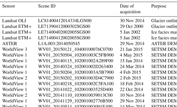
Table 1.Scenes used in glacier outline delineation, ASTER DEM generation, SRTM ice facies mask generation and by the Polar Geospatial Center in the generation of SETSM DEMs.
Sensor Scene ID Date of Purpose
acquisition
Landsat OLI LC81400412014334LGN00 30 Nov 2014 Glacier outlines Landsat ETM+ LE71390412000302SGS00 29 Oct 2000 Glacier outlines Landsat ETM+ LE71400402002005SGS00 5 Jan 2002 Ice facies mask Landsat ETM+ LE71400412002005SGS00 5 Jan 2002 Ice facies mask
ASTER L1A.003:2014050545 29 Nov 2014 ASTER DEM
WorldView 3 WV03_20150121_10400100076C0700 21 Jan 2015 SETSM DEM WorldView 1 WV01_20150504_102001003C5FB900 4 May 2015 SETSM DEM WorldView 1 WV01_20140115_102001002A289F00 15 Jan 2014 SETSM DEM WorldView 1 WV01_20140324_102001002D263400 24 Mar 2014 SETSM DEM WorldView 1 WV01_20150204_102001003A5B7900 4 Feb 2015 SETSM DEM WorldView 2 WV02_20150202_103001003D4C7900 2 Feb 2015 SETSM DEM WorldView 1 WV01_20140218_102001002C5FA100 18 Feb 2014 SETSM DEM WorldView 1 WV01_20141022_102001003525D400 22 Oct 2014 SETSM DEM WorldView 2 WV02_20141110_1030010039013C00 10 Nov 2014 SETSM DEM WorldView 1 WV01_20141129_102001002776B500 29 Nov 2014 SETSM DEM WorldView 1 WV01_20140514_102001003001E400 14 May 2014 SETSM DEM
3 Data sources and methods 3.1 Data sources
3.1.1 Digital elevation models
Our reference elevation dataset across all three catchments is the Shuttle Radar Topography Mission (hereafter SRTM) version 3.0, non-void-filled, 1 arcsec digital elevation model (hereafter DEM). The main objective of the SRTM mission was to obtain single-pass interferometric Synthetic Aperture Radar (SAR) imagery to be used for DEM generation on a near-global scale (56◦S to 60◦N – 80 % of the planet’s sur-face) with targeted horizontal and vertical accuracies of 16 and 20 m, respectively, although Farr et al. (2007) report hor-izontal and vertical accuracies of better than 10 m for most regions globally. This dataset was acquired in February 2000 and was released at 30 m resolution in late 2014 (USGS, 2016). The SRTM data we used were acquired by a 5.6 cm C-band radar system.
Our 2014/2015 elevation dataset comprises a number of high-resolution (8 m grid) DEMs generated by Ohio State University and distributed online by the Polar Geospatial Center at the University of Minnesota that provide cover-age of an extended area around the Everest region (Table 1). These stereo-photogrammetric DEMs have been generated using a Surface Extraction with TIN-based Search-space Minimization (hereafter SETSM) algorithm from World-View 1, 2 and 3 imagery (Noh and Howat, 2015). The SETSM algorithm is designed to automatically extract a stereo-photogrammetric DEM from image pairs using only the Rational Polynomial Coefficients (RPCs) as geomet-ric constraints. The geolocation accuracy of RPCs without
ground control for WorldView 1 and 2 data is 5 m (Noh and Howat, 2015) which may ultimately result in matching fail-ure. The SETSM algorithm updates RPCs to mitigate this error and produces DEMs with an accuracy of±4 m in X,
Y andZdirections (Noh and Howat, 2015). SETSM DEMs are gap filled using a natural neighbour interpolation; we re-moved these pixels before DEM differencing and calculating glacier mass balance.
Over two small areas of the Dudh Koshi (over the lower reaches of the Bhote Kosi and Melung glaciers), the SETSM DEMs contained data gaps. To complete coverage of DEMs over these glaciers we generated ASTER (Advanced Space-borne Thermal Emission and Reflection Radiometer) DEMs and used the surface to cover elevation bands across the glaciers for which no data were available from the SETSM grids. We used ERDAS Imagine (2013) to generate ASTER DEMs with ground control points (GCPs) matched between features in the ASTER imagery and the high-resolution im-agery available in Google Earth. We used a large number of GCPs (45) and tie points (> 75) to minimise the root mean square error of GCP positions. All SETSM and ASTER DEMs were resampled to a 30 m resolution to match that of the SRTM data before any differencing was carried out. 3.1.2 Glacier outlines
The-matic Mapper Plus (ETM+) sensor and thus has a single 15 m resolution panchromatic band and six 30 m multispec-tral bands. The 2014 scene was acquired by the Operational Land Imager (OLI) sensor and has a single 15 m panchro-matic band as well as eight 30 m multispectral bands. Both scenes were pan-sharpened to match the resolution of the multispectral bands to that of the panchromatic band before glacier outlines were adjusted. Adjustments were limited to correcting changes in glacier frontal position and changes along the lateral margins because of surface lowering. 3.2 DEM correction
3.2.1 Stereoscopic DEMs
We followed the three-step correction process of Nuth and Kääb (2011), through which biases inherent in stereoscopic DEMs can be corrected. We assessed and corrected where necessary for (i) a mismatch in the geolocation of the mod-ern DEMs versus the reference SRTM dataset (inx,yandz
direction), (ii) the existence of an elevation dependant bias and (iii) biases related to the acquisition geometry of the data. Each step was taken individually, so that separate er-ror terms could be understood, rather than bundling them together as multiple-regression-based adjustments as previ-ous studies have done, such as Racoviteanu et al. (2008) and Peduzzi et al. (2010). Corrections applied to DEMs for which any one of the three biases were present included shifting DEM corner coordinates, simple vertical shifting through addition or subtraction, and the fitting of linear and polynomial trends depending on the spatial variability of el-evation differences across DEMs and through their eleva-tion ranges. Acquisieleva-tion of geometry-related biases (along or cross satellite track) were detected in two SETSM strips (Table 3) and both ASTER scenes and were corrected for using linear trends fitted through difference data. DEM co-registration was carried out following the conversion of SETSM elevation data to geoid heights using the Earth Grav-itational Model (EGM) 2008 grid available from the National Geospatial-Intelligence Agency. Table 2 shows a summary of DEM difference data over stable, off-glacier areas before and after DEM coregistration.
3.2.2 SRTM DEM correction
Some studies have shown that the SRTM dataset may under-estimate glacier surface elevations because of C-band radar wave penetration into snow and ice (Rignot et al., 2001). Kääb et al. (2012) assessed the magnitude of C-band penetra-tion over various test sites in the Himalayas and over different ice facies (clean ice, snow and firn) by extrapolating ICESat vs. SRTM glacier elevation differences back to the SRTM ac-quisition date, showing penetration estimates of several me-tres. To account for this bias, we have corrected the SRTM dataset using the penetration estimates of Kääb et al. (2012),
after generating a mask for clean ice, firn and snow cover us-ing the most suitable Landsat ETM+scenes (Table 1) avail-able around the acquisition date of the SRTM dataset. We applied a correction to the SRTM DEM of+4.8 m over areas of firn/snow and+1.2 m over areas of clean ice (see Table S2 of Kääb et al., 2012). We do not apply any penetration cor-rection over debris-covered areas given the uncertainty ex-pressed by Kääb et al. (2012) about the influence of possibly greater than average snowpack depth at the point of ICESat acquisition and the properties of the snowpack at the point of SRTM data acquisition on their penetration estimate.
Berthier et al. (2006) suggested that the extreme topog-raphy present in mountain regions is poorly replicated in coarse-resolution DEMs such as the SRTM DEM. Differ-ent studies have applied positive or negative corrections to the SRTM DEM (Berthier et al., 2007; Larsen et al., 2007), depending on the severity of the terrain at their respective study sites. Inspection of DEM differences across the study site showed no clear relationship between elevation differ-ences and altitude (see Fig. S1); thus no elevation-dependant correction was applied.
3.2.3 Gap filling and outlier filtering
Once DEMs had been co-registered and corrected for present biases, DEMs were differenced to yield surface elevation change data. To remove outlying values, we firstly excluded obviously incorrect difference values (exceeding ±120 m) and then followed the approach of Gardelle et al. (2013) in using the standard deviation of DEM difference data to clas-sify probable outliers. We removed values exceeding 3 stan-dard deviations. Such outlier definitions are justified in areas of shallow slope and high image contrast when DEM quality is generally high (Ragettli et al., 2016), but could be consid-ered lenient where featureless surfaces, for example snow-covered areas of accumulation zones, might lead to poor ele-vation data deriele-vation and limit the accuracy of stereoscopic DEMs. Noh and Howat (2015) show how the iterative ap-proach of the SETSM algorithm and the high spatial and ra-diometric resolution of WorldView imagery preclude such an issue, and we therefore consider a 3 standard deviation threshold appropriate.
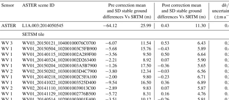
Table 2.Mean differences and the standard deviation associated with off-glacier elevation difference data between ASTER, SETSM and SRTM DEMs before and after the DEM correction process. The uncertainty associated with DEM difference data (sum of standard error estimates for each 100 m elevation bin of difference data) is also listed for each SETSM and ASTER DEM.
Sensor ASTER scene ID Pre correction mean Post correction mean dh/dt
and SD stable ground and SD stable ground uncertainty differences Vs SRTM (m) differences Vs SRTM (m) (±m a−1)
ASTER L1A.003:2014050545 −64.12 25.99 0.43 11.30 0.47
SETSM tile
WV 3 WV03_20150121_10400100076C0700 −6.07 11.54 0.53 6.43 0.25
WV 1 WV01_20150504_102001003C5FB900 −5.68 15.76 −0.43 5.89 0.40
WV 1 WV01_20140115_102001002A289F00 −3.56 9.50 0.50 6.64 0.27
WV 1 WV01_20140324_102001002D263400 −2.21 8.92 0.07 5.90 0.33
WV 1 WV01_20150204_102001003A5B7900 −1.26 17.50 −0.36 5.65 0.31
WV 2 WV02_20150202_103001003D4C7900 −3.80 12.34 −0.03 6.56 0.29
WV 1 WV01_20140218_102001002C5FA100 −2.00 9.80 −0.23 6.71 0.28
WV 1 WV01_20141022_102001003525D400 −9.54 16.50 0.36 6.89 0.35
WV 2 WV02_20141110_1030010039013C00 −2.89 9.83 0.07 5.87 0.15
WV 1 WV01_20141129_102001002776B500 −5.72 8.31 0.16 4.76 0.18
WV 1 WV01_20140514_102001003001E400 −3.51 10.12 −0.26 5.91 0.26
3.3 Uncertainty
3.3.1 DEM differencing uncertainty
Our elevation change uncertainty estimates have been calcu-lated through the derivation of the standard error(E1h)– the standard deviation of the mean elevation change – of 100 m altitudinal bands of elevation difference data (Gardelle et al., 2013; Ragettli et al., 2016):
E1h= σstable
√
N , (1)
whereσstable is the standard deviation of the mean elevation
change of stable, off-glacier terrain, and N is the effective number of observations (Bolch et al., 2011).Nis calculated through the following:
N =Ntot×PS
2d , (2)
whereNtotis the total number of DEM difference data points, PS is the pixel size anddis the distance of spatial autocorre-lation. We follow Bolch et al. (2011) in estimatingdto equal 20 pixels (600 m). E1h for each DEM is the sum of stan-dard error estimates of each altitudinal band (Gardelle et al., 2013).
We have also considered whether the different acquisition dates of WorldView imagery (Table 1) have led to the sam-pling of seasonal glacier surface elevation variations caused by a remnant snowpack (e.g. Berthier et al., 2016). Such a bias should be partly corrected for during vertical DEM ad-justment using off-glacier terrain assuming a similar snow-pack thickness on and off-glacier (Wang and Kääb, 2015). Two overlapping SETSM DEMs (ending FA100 and 3C00 in
Table 1) have been generated from WorldView imagery ac-quired before and after the summer monsoon (when glaciers receive most accumulation) of 2014; thus any spatially con-sistent vertical differences may show a remnant snowpack that would cause an elevation bias. The difference between these two SETSM DEMs over the Bamolelingjia and G1 glaciers is slight (mean 0.69 m,σ 3.81 m), but we cannot be sure that these differences represent a region-wide average. We have incorporated the mean elevation difference of these SETSM DEMs over glacier surfaces (dZseason)into our over-all uncertainty budget. We summed different sources of error quadratically to calculate our overall uncertainty (σdh/dt)
as-sociated with DEM difference data:
σdh
dt
=
q
E1h2 +dZ2
season. (3)
σdh/dtis then weighted depending on the hypsometry of each
glacier, giving a glacier-specific measure of elevation change uncertainty that considers the spatially non-uniform distribu-tion of uncertainty (Ragettli et al., 2016).
3.3.2 Glacier area change uncertainty
sug-gest the total measurement uncertainty in glacier area be-tween 2000 and 2015 image sets was±0.04 km2a−1.
Area-weighted, glacier-specific uncertainty estimates are given in Table S3.
3.4 Hypsometric analyses and elevation range normalisation
Glacier hypsometry, the distribution of a glacier area over altitude, is governed by valley shape, relief and ice-volume distribution (Jiskoot et al., 2009). It is important for the long-term glacier response because it defines the distribution of mass with elevation and thus determines how the glacier re-sponds to changes in elevation-dependent temperature (Fur-bish and Andrews, 1984). To assess glacier hypsometry, we used the aforementioned glacier outlines and the SETSM DEMs, which offer better data coverage than the non-void-filled SRTM dataset, to split these glacier extents into seg-ments covering 100 m elevation ranges, and calculated the area of each segment. We followed the approach of Jiskoot et al. (2009) to categorise each glacier or the population of glaciers in each catchment according to a hypsometric index (HI), where
HI=(Hmax−Hmed)
(Hmed−Hmin)
(4)
andHmaxandHminare the maximum and minimum eleva-tions of the glacier, and Hmed is the median elevation that divides the glacier area in half (Jiskoot et al., 2009). Glaciers were grouped into five HI categories: 1 is HI <−1.5, very top heavy; 2 is HI−1.2 to−1.5, top heavy; 3 is HI−1.2 to 1.2, equidimensional; 4 is HI 1.2 to 1.5, bottom heavy; and 5 is HI > 1.5, very bottom heavy. Top-heavy glaciers store more ice at higher elevation, for example in broad accumulation zones, whereas bottom heavy glaciers have small accumula-tion zones and long tongues.
To construct elevation change and glacier hypsometry curves for the 32 glaciers in our sample, we have normalised the elevation range of each glacier following the method of Arendt et al. (2006):
Hnorm=
(H−Hmin)
(Hmax−Hmin), (5)
whereHminandHmaxare the elevations of the glacier
termi-nus and the elevation maximum of each glacier. This normal-isation process allows for a direct comparison of elevation changes and glacier hypsometry regardless of termini eleva-tion. Surface elevation change and glacier hypsometry curves are presented in Figs. 5 and 6.
3.5 Mass loss calculations
A conversion factor of 850 kg m−3 was used to account for the density of glacier ice for all glaciers in the sample (Huss,
2013). We assigned an additional 7 % to mass loss uncer-tainty estimates to account for error in the density conver-sion (Huss, 2013). The mass loss estimates generated for lacustrine-terminating glaciers are slight underestimates be-cause, with no information available on bed topography, we cannot account for ice that has been replaced by wa-ter during lake expansion. Mass balance estimates for these glaciers therefore only incorporate aerial mass loss from the 2000 calving front, up-glacier. We also acknowledge that our surface-lowering estimates incorporate any upward or down-ward flow of ice resulting from, for example, compressional flow over a zone of transition from active to inactive ice. We do not quantify emergence velocity as the ice thickness and surface velocity data required to do so (Immerzeel et al., 2014) are not available for an adequate number of glaciers in our sample.
3.6 Estimation of ELAs
We follow the approach of Braithwaite and Raper (2010) in using the median altitude of each glacier, information avail-able in the RGI, to estimate the ELA of glaciers in our sample. Such an approach is most appropriate for glaciers in a state of balanced mass budget (Braithwaite and Raper, 2010; Braithwaite, 2015); thus the ELA estimates produced using this method could be considered an underestimate of modern-day ELAs given the negative state of mass balance of the majority of Himalayan glaciers. However, without mea-sured mass balance records of adequate length against which to compare this or other (Braithwaite, 2015) ELA estima-tion methods, we take it as the best available approach. This is a method that has previously been employed in the Hi-malayas (Zhao et al., 2016), although we also note that this method cannot account for the input of avalanched material from steep valley walls – a substantial source of accumu-lation for Himalayan glaciers (Benn and Lehmkuhl, 2000). To estimate prospective future ELAs in response to temper-ature increases, we used vertical tempertemper-ature gradients of
−8.5◦C km−1for the Pumqu catchment (Kattel et al., 2015) and −5.4◦C km−1 for the Dudh Koshi and Tama Koshi catchments (Immerzeel et al., 2014) to calculate prospec-tive ELA shifts given different warming scenarios. We cal-culated ELAs for projected minimum, mean and maximum temperature increases under the four main RCP (Representa-tive Concentration Pathways) scenarios outlined in the IPCC AR5 working group report (Collins et al., 2013).
4 Results
4.1 Glacier mass balance
The mean mass balance of all 32 glaciers in our sample was
surface lowering through the altitudinal range of highlighted glaciers (Figs. 5 and 6). The mean mass balance of glaciers in catchments either side of the orographic divide are not markedly different, however.
Mean glacier mass balance (including land and lacustrine-terminating glaciers) was −0.51±0.22 m w.e. a−1 in the Tama Koshi catchment,−0.58±0.19 m w.e. a−1in the Dudh Koshi catchment and −0.61±0.24 m w.e. a−1 for glaciers flowing into the Pumqu catchment over the study pe-riod. The mean mass balance of nine lacustrine-terminating glaciers was −0.70±0.26 m w.e. a−1. This was 32 % more negative than land-terminating glaciers (mean mass bal-ance of −0.53±0.21 m w.e. a−1) we include in our sam-ple. The lowest mass loss rates occurred over debris-free glaciers at high altitude (5600–6200 m a.s.l) in the Pumqu catchment. The mean mass balance of these glaciers was
−0.25±0.22 m w.e. a−1(Table S2) over the study period.
In-dividual glacier mass balance estimates can be found in the Supplement.
4.2 Glacier surface lowering
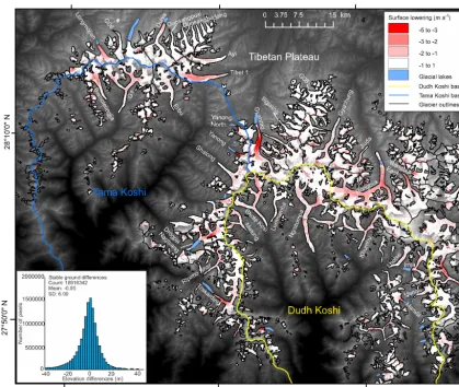
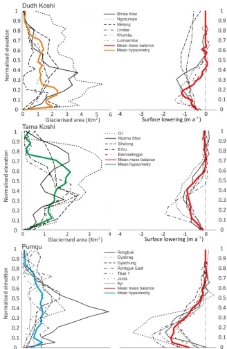
The altitude at which maximum surface-lowering rates oc-curred differed depending only on glacier terminus type (Figs. 5 and 6). Across all three catchments, substan-tial surface lowering was pervasive over the middle por-tions of larger, land-terminating glaciers (Fig. 2). In the Dudh Koshi, surface-lowering rates are at their highest (−1.06±0.10 m a−1) around 5200 m a.s.l., although sim-ilar surface-lowering rates occurred between 5100 and 5300 m a.s.l (Fig. 5). In the Tama Koshi the highest rates of surface lowering (−1.08±0.12 m a−1) occurred at around
5400 m a.s.l (Fig. 5). In the Pumqu catchment, the highest mean surface-lowering rates again occurred between 5300 and 5400 m a.s.l.; the mean surface-lowering rate at this alti-tude was−1.62±0.14 m a−1over the study period. Surface-lowering rates over glaciers in the Pumqu catchment were higher than those in the Tama Koshi and Dudh Koshi catch-ments (Fig. 5) up to 5700 m a.s.l. (−1.24±0.21 m a−1at this altitude). Of note is the surface lowering over clean-ice areas high up on glaciers such as Ngozumpa, Rongbuk, Gyabrag and Bhote Kosi (Fig. 2). Surface lowering extended into trib-utary branches and the cirques of these largest glaciers. In-dividual glaciers showed much greater surface lowering, par-ticularly in the Pumqu catchment. Gyabrag glacier lost an ex-ceptional−3.33±0.28 m a−1between 5300 and 5400 m a.s.l (Fig. 5).
The maximum surface-lowering rates
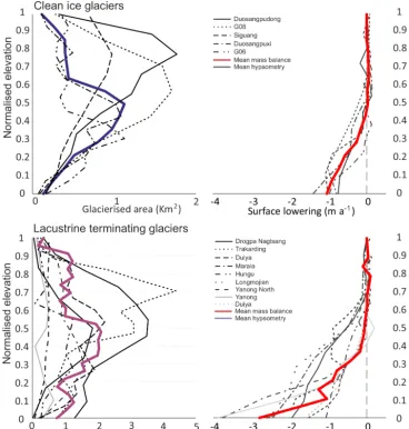
(−2.79±0.29 m a−1) occurred at the lowest elevations (between 4700 and 4900 m a.s.l) of lacustrine-terminating glaciers (Fig. 6). These nine glaciers all showed a linear surface-lowering gradient. We calculate the lowering gradi-ent as surface elevation change per 100 m [m a−1(100 m)−1] vertical elevation change below the ELA. Lacustrine-terminating glaciers showed a lowering gradient of
0.30 m a−1(100 m)−1 over the study period. The lowering gradient of land-terminating glaciers was non-linear. Surface lowering was negligible around the terminus of most land terminating glaciers, with enhanced ice loss occurring further up-glacier where debris cover may have been thin or patchy. Lowering gradients for the area of land-terminating glaciers between the ELA and the altitude of maximum ice loss were 0.59, 0.66 and 0.38 m a−1(100 m)−1 for glaciers in the Pumqu, the Dudh Koshi and Tama Koshi catchments, respectively. Clean-ice glaciers also showed a linear lowering gradient – 0.77 m w.e. a−1(100 m)−1. 4.3 Glacier area changes and hypsometry 4.3.1 Total area changes
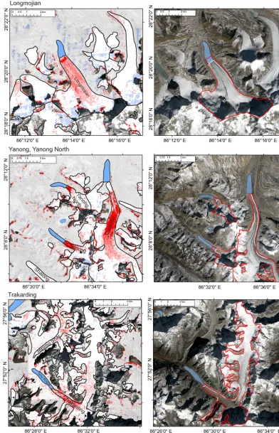
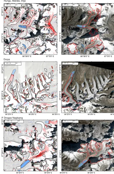
Two different patterns of ice area loss occurred over the study area during the last 15 years. Lacustrine-terminating glaciers and clean-ice glaciers all lost ice around their termini/calving fronts (Figs. 3 and 4) as glacial lakes expanded and termini receded. On average, lacustrine terminating glaciers each lost 0.54±0.07 km2 of ice (3.58 % of their total area) over the 15-year study period. Drogpa Nagtsang reduced in size by 2.37 km2 (9.12 % of its total area; Table S3) as the associ-ated rapidly forming lake expanded. Clean-ice glaciers lost 0.09±0.03 km2 of ice (1.31 % of their total area) on aver-age.
Land-terminating glaciers lost little area as their surfaces lowered instead of their termini retreating. In the Tama Koshi and Dudh Koshi catchments, and in the Pumqu catchment, land-terminating glaciers lost a mean of 0.14±0.12 km2 (0.50 % of their total area), 0.09±0.13 km2(0.60 % of their total area) and 0.41±0.12 (1.77 % of their total area) of ice, respectively. Over these glaciers, any ice area loss was concentrated up-glacier, where their lateral margins dropped down inner moraine slopes and glacier tongues narrowed slightly.
Overall, our sample of glaciers lost 0.12±0.04 % of their total area per year over the study period. This figure is iden-tical to that of Bolch et al. (2008), who assessed area change over a smaller number of the same glaciers in our sample between 1962 and 2005. The annual area change rate we cal-culated is lower than those estimated by Thakuri et al. (2014) and references within. Thakuri et al. (2014) calculated a me-dian annual surface area change rate of−0.42±0.06 % a−1
in the Dudh Koshi catchment between 1962 and 2011. How-ever, Thakuri et al. (2014) document area change over a num-ber of smaller glaciers that are free of debris cover and there-fore readily advance or retreat in response to climatic change; thus our estimates are not directly comparable.
Figure 2.Glacier surface elevation change over the study area between 2000 and 2014/15. Also shown is a summary of off-glacier terrain differences. Areas of no data show the ASTER GDEM underlay.
glaciers of the Dudh Koshi catchment and the Pumqu catch-ment are typically very bottom heavy, with average HI scores of 2.63 and 2.34 (Table S1). Glacier hypsometry is concentrated between 4800 and 5500 m (Fig. 5) for the Dudh Koshi catchment and between 5600 and 6500 m in the Pumqu catchment. Notable exceptions are the Khumbu and Ngozumpa glaciers which store ice in broad accumula-tions zones above 7000 m (Tables S1 and S2). The major-ity of glaciers in the Tama Koshi have an equidimensional hypsometry (mean HI of 1.14), with most ice stored be-tween 5300 and 5800 m. Glaciers in the Tama Koshi have broader accumulation basins than in the Dudh Koshi catch-ment, and the main glacier tongues are formed of multiple, smaller tributaries flowing from higher altitude in a number of cases (Fig. 1). The mean hypsometry (Fig. 6) of lacustrine-terminating glaciers shows no distinctive morphology as the sample is composed of glaciers from all three catchments in the study area. Clean-ice glaciers have a mean HI of 1.18 and could therefore be summarised as equidimensional, but the morphology of the five glaciers we assess is highly
vari-able (see Tvari-able S3). In complete contrast to debris-covered glaciers, their ice is stored at higher mean altitudes on aver-age, primarily between 6000 and 6500 m (Fig. 6).
Figure 5.Surface elevation change and glacier hypsometry curves for all land terminating glaciers in the three different catchments of the study area.
5 Discussion
5.1 Variability in rates of ice loss across the orographic divide
The mean mass balance estimates we have derived for glaciers situated in catchments north and south of the main orographic divide are not markedly different. However, the
Figure 6.Surface-lowering and glacier hypsometry curves for clean ice and lacustrine-terminating glaciers in the study area.
of the difference in the rates of surface lowering across the range divide.
The Indian summer monsoon delivers a large proportion of total annual precipitation (up to 80 % of the total an-nual amount) to the Everest region of Nepal, resulting in high glacier sensitivity to temperature (Fujita, 2008; Sakai et al., 2015). The extreme topography in this region and the location of the orographic divide perpendicular to the prevailing monsoon result in rainfall peaks that are offset from the maximum elevations, with greatest rainfall occur-ring to the south of the divide and decreasing to the north across the Everest region (Bookhagen and Burbank, 2010; Wagnon et al., 2013). Around 449 mm a−1 of rainfall falls at the Pyramid research station (5000 m a.s.l.) at Khumbu Glacier (Salerno et al., 2015), whereas Dingri on the Ti-betan Plateau (4300 m a.s.l.) to the north is much drier with 263±84.3 mm a−1 of rainfall annually (Yang et al., 2011).
Snowfall may follow a similar across-range gradient to
rain-fall, although falling snow may be carried further into the range by prevailing winds from the south. However, no re-liable measurements of snowfall exist in this region with which to compare these trends. The north–south precipita-tion gradient across the orographic divide promotes differ-ences in the response of these glaciers to climate change, such that those to the north are relatively starved of snow accumulation (Owen et al., 2009) and exposed to greater in-coming radiative fluxes under generally clearer skies. Owen et al. (2009) suggest that this precipitation gradient resulted in greater glacier sensitivity to climate change on the north-ern slopes of the Himalayas during the Late Quatnorth-ernary, with asymmetric patterns of ELA rise occurring since the Last Glacial Maximum (LGM).
Koshi catchment, increases in minimum (+0.07◦C a−1), maximum (+0.009◦C a−1)and mean (+0.044◦C a−1)
an-nual air temperatures above 5000 m a.s.l. were observed be-tween 1994 and 2013 (Salerno et al., 2015). At Dingri on the Tibetan Plateau, 60 km north-east of Mt Everest, increases in minimum (+0.034◦C a−1), maximum (+0.041◦C a−1)and mean (+0.037◦C a−1)annual air temperatures occurred over the same period (Salerno et al., 2015). Yang et al. (2011) also show a longer-term increase in the mean annual air tempera-ture at Dingri, as do Shrestha et al. (1999) across the southern flank of the greater Himalayas. Between 1959 and 2007, the mean annual air temperature increased by 0.06◦C a−1at Dgri (Yang et al., 2011). Shestha et al. (1999) calculated an in-crease in the mean annual air temperature of 0.057◦C a−1 be-tween 1971 and 1994 across a number of sites in the greater Himalayas.
The snow-line altitude also appears to have increased re-cently on the southern flank of the Himalaya; Thakuri et al. (2014) showed a rapid ascent of the snow-line altitude in the Dudh Koshi between 1962 and 2011 (albeit through doc-umenting transient snow lines from single scenes acquired at each epoch), and Khadka et al. (2014) suggest declin-ing snow cover over the winter and sprdeclin-ing months in the glacierised altitudinal ranges of the Tama Koshi catchment, between 2000 and 2009; a factor that may influence lation rates. Kaspari et al. (2008) showed decreasing accumu-lation recorded in an ice core collected from East Rongbuk Glacier Col (6518 m a.s.l.) on the northern side of Mt Everest between the 1970s and 2001.
We suggest that the north–south orographic precipitation gradient across the main divide may have caused greater surface-lowering rates on glaciers in the Pumqu catchment than those glaciers to the south over the study period. We also suggest that measured, contemporary increases in air tem-perature, observations of increasing snow-line altitude and declining accumulation are likely to enhance glacier mass loss across the range in future, but considerable unknown fac-tors remain in the temporal evolution of debris cover extent and thickness (Thakuri et al., 2014), the strength of the sum-mer monsoon in coming decades (e.g. Boos and Storelvmo, 2016), and the expansion or shrinkage of glacial lakes (see Sect. 5.3), all of which could additionally influence future glacier mass balance.
5.2 Comparison of mass balance estimates with other studies
[image:14.612.323.531.106.359.2]Several other studies have generated geodetic mass balance estimates for glaciers of the Everest region over several different time periods. Bolch et al. (2011) generated bal-ance estimates of−0.32±0.08 and−0.79±0.52 m w.e. a−1 for 10 glaciers to the south and west of Mt Everest over the periods 1970–2007 and 2002–2007, respectively. Nuimura et al. (2012) calculated a regional mass balance of−0.45±0.25 m w.e. a−1for 97 glaciers across the region
Table 3.Mass balance estimates (from geodetic and altimetric stud-ies) for the broader Everest region and comparable subregions/ catchments.
Time period Mass balance Study
and area estimate
(m w.e. a−1)
Dudh Koshi
1970–2007 −0.32±0.08 Bolch et al. (2011) 1992–2008 −0.45±0.25 Nuimura et al. (2012) 2002–2007 −0.79±0.52 Bolch et al. (2011) 2000–2015 −0.58±0.19 This study
Pumqu (Tibetan Plateau)
1974–2006 −0.40±0.27 Ye et al. (2015) 2003–2009 −0.66±0.32 Neckel et al. (2014) 2000–2015 −0.61±0.24 This study
Tama Koshi
2000–2015 −0.51±0.22 This study
Everest region
1999–2011 −0.26±0.13 Gardelle et al. (2013) 2003–2008 −0.39±0.11 Kääb et al. (2012) 2000–2015 −0.52±0.22 This study
over the period 1992–2008. Kääb et al. (2012) estimated a mass balance of −0.39±0.11 m w.e. a−1 for a 3◦×3◦ cell centred on the Everest region between 2003 and 2008. Gardelle et al. (2013) calculated a slightly less negative mass balance of−0.26±0.13 m w.e. a−1between 1999 and 2011, although the SRTM penetration correction applied by Gardelle et al. (2013) may have caused a bias towards a less negative mass balance (Kääb et al., 2012; Barundun et al., 2015). The regional mass balance of−0.52±0.22 m w.e. a−1 that we have calculated suggests that the mass loss rates mea-sured by Nuimura et al. (2012) and Kääb et al. (2012) have been sustained and possibly increased in recent years (Ta-ble 3), as Bolch et al. (2011) also suggest.
5.3 The influence of glacial lakes on glacier mass balance
Only Nuimura et al. (2012) have directly compared mass loss rates of lacustrine and land-terminating glaciers in the study area, showing faster surface-lowering rates over Imja and Lumding glaciers in the Dudh Koshi catchment. Our data confirm that lacustrine-terminating glaciers can indeed lose ice at a much faster rate than land-terminating glaciers. The variability in the mass balance of the nine lacustrine-terminating glaciers (Fig. 6) we highlight suggests the fastest mass loss rates occur in the later stages of lake development. Glaciers such as the Yanong and Yanong North, in the Tama Koshi catchment, sit behind large proglacial lakes and are in a state of heavily negative mass balance (−0.76±0.18 and
−0.62±0.25 m w.e. a−1, respectively). Their surfaces low-ered by 3 m a−1 or more over their lower reaches (Fig. 6) over the study period. These glaciers are now relatively small and steep and no longer possess a debris-covered tongue, and so may represent the end product of debris-covered glacier wastage described by Benn et al. (2012). In con-trast, glaciers such as Duiya, in the Pumqu catchment, cur-rently has only a small lake at its termini, showed mod-erate area losses (0.5 km2 or 4.28 % of its total area) and moderately negative mass balance (−0.45±0.13 m w.e. a−1)
over the study period. Continued thinning of the terminal regions of glaciers with smaller glacial lakes would lead to a reduction in effective pressure, an increase in longi-tudinal strain and therefore flow acceleration (Benn et al., 2007). The retreat of the calving front up-valley into deeper bed topography may also increase calving rates (Benn et al., 2007), and a combination of both of these processes would lead to enhanced ice loss. Very few surface velocity data exist for lacustrine-terminating debris-covered glaciers. Only Quincey et al. (2009) measured high surface veloci-ties (25 m a−1or more) over Yanong glacier (their Fig. 4d), suggesting it is possible for lacustrine-terminating glaciers to become more dynamic in the later stages of lake devel-opment in the Himalayas. Conversely, Thakuri et al. (2016) have shown flow deceleration of glaciers that coalesce to ter-minate in Imja Tsho over the period 1992–2014 and sug-gest that reduced accumulation caused by decreasing pre-cipitation is responsible for diminishing surface flow on this glacier. Clearly, more expansive investigation into the evolv-ing dynamics of lacustrine-terminatevolv-ing glaciers in the Hi-malayas is required if we are to better understand their po-tential future mass loss.
5.4 Glacier stagnation
A number of studies (Luckman et al., 2007; Scherler et al., 2008, 2011; Quincey et al., 2009) have shown how many glaciers in the Everest region appear to be predominantly stagnant, with large parts of the long, debris-covered glacier tongues in the area showing little to no flow. Watson et
al. (2016) have documented an increasing number and to-tal area of supraglacial melt ponds over a number of the same glaciers studied by Quincey et al. (2009) in the Dudh Koshi catchment (Khumbu, Ngozumpa, Lhotse, Imja and Ama Dablam), since the early 2000s. Over these glaciers, our data show a very distinctive surface-lowering pattern (Fig. 2), with localised, heterogenous surface lowering ap-pearing to mirror the distribution of large supraglacial ponds and ponds networks. This ice loss pattern is prevalent on the Erbu, Gyachung, Jiuda, Shalong and G1 glaciers (Fig. 2), and high-resolution imagery available on Google Earth shows that these glaciers also have well-developed networks of supraglacial ponds. We would therefore suggest that large parts of the biggest glaciers in the Tama Koshi catchment and in the Pumqu catchment are also stagnant and may see increasing supraglacial meltwater storage in the future, simi-lar to that documented by Watson et al. (2016).
5.5 Susceptibility of glaciers to future mass loss ELA ascent in response to temperature increases
The coincidence of maximum surface-lowering rates with the altitude of maximum hypsometry in the Dudh Koshi ment (Fig. 5) suggests large glacier mass losses in this catch-ment. Sustained and prolonged mass loss may lead to a bi-modal hypsometry here, with the physical detachment of debris-covered glacier tongues and their high-elevation ac-cumulation zones a possibility (Rowan et al., 2015; Shea et al., 2015). Surface-lowering maxima in the Tama Koshi catchment presently occur at a slightly lower elevation range than the main hypsometric concentration, and across lower reaches of glacier tongues in the Pumqu catchment.
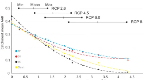
Figure 7 shows projected AARs, averaged across each catchment, in response to different levels of temperature rise. These predictions are based on published lapse rates (Im-merzeel et al., 2014; Kattel et al., 2015) that may be spa-tially variable and assume no changes in precipitation type or amount or any variability in the contribution of avalanches to accumulation.
Figure 7.Projected AARs (averaged across each catchment) based on different scenarios of temperature increase relative to the present day and accompanying ELA rise. Temperature rise scenarios have been used from the IPCC AR5 Working Group report. P is Pumqu, DK is Dudh Koshi, TK is Tama Koshi and Clean is clean-ice glaciers. Each point represents a projected AAR given minimum, mean or maximum temperature rise under each RCP scenario.
effects of a rise in ELA on glacier mass balance, with AAR adjustment occurring more gradually (Fig. 7). AARs could decrease to 0.27 or 0.17 in the Dudh Koshi and to 0.29 or 0.18 in the Pumqu catchment. ELA rise in response to this particular warming scenario would mean a 12–30 % increase in the total glacierised area below the ELA in the Pumqu catchment, a 24–61 % increase in the Tama Koshi catchment and a 23–40 % increase in the Dudh Koshi catchment. Should more substantial temperature increases occur (> 2◦C warm-ing), AARs could reduce to zero on a number of individual glaciers, and the ELA could rise to near-maximum glacier al-titudes in the Tama Koshi catchment. Clean-ice glacier AAR adjustment may be rapid given their limited altitudinal range (Fig. 7).
Glacier AAR is a parameter strongly related to long-term mass balance for typical alpine glaciers (König et al., 2014), although the effect of a diminishing AAR may be dampened on Himalayan glaciers given the large input of avalanche material derived from high surrounding headwalls (Iturrizaga, 2011). Since data on the rates of avalanching in high-mountain environments such as the Himalayas are sparse (Benn and Lehmkuhl, 2000), the impact of predicted AAR reduction remains somewhat uncertain.
6 Conclusions
DEM differencing has revealed substantial mass loss from many large, debris-covered glaciers in the central Hi-malayas over the last 15 years. Geodetic mass balance estimates have been calculated for 32 glaciers across three different catchments around the Everest region. We found similarly negative mass budgets for glaciers flow-ing onto the southern flank of the Himalayas, in the
Tama Koshi (−0.51±0.22 m w.e. a−1) and Dudh Koshi (−0.58±0.19 m w.e. a−1) catchments, and in the Pumqu
catchment (−0.61±0.24 m w.e. a−1).
The division of our sample of glaciers depending on their terminus type shows contrasting mass loss rates be-tween land and lacustrine-terminating glaciers. The mean mass balance of nine lacustrine-terminating glaciers we assessed was −0.70±0.26 m w.e. a−1, 32 % more nega-tive than land-terminating glaciers (mean mass balance of −0.53±0.21 m w.e. a−1). The mass balance of nine lacustrine-terminating glaciers ranged from−0.91±0.22 to
−0.45±0.13 m w.e. a−1 and we would suggest that glacial lakes in the region are at different stages of expansion. Ac-celerating mass loss is likely from several of these lacustrine-terminating glaciers, the termini of which will retreat into deeper lake water.
Surface-lowering curves show that the maximum-lowering rate (−1.62±0.14 m a−1 between 5300 and 5400 m.a.s.l.)
of glaciers in the Pumqu catchment was well above the maximum-lowering rate of glaciers flowing south of the orographic divide (−1.06±0.10 m a−1 between 5200 and 5300 m a.s.l. in the Dudh Koshi catchment,
−1.08±0.12 m a−1 between 5200 and 5300 m a.s.l. in the Tama Koshi catchment), and that glaciers in the Pumqu catchment are losing ice over a much broader altitudinal range than their south-flowing counterparts. We suggest that the across-range contrast in annual precipitation amount, combined with rising mean air temperatures over recent decades may have caused greater ice loss rates from the north-flowing glaciers.
Predicted warming in the Everest region will lead to in-creased ELAs and, depending on glacier hypsometry, sub-stantial increases in the size of ablation areas. We show that glaciers of the Tama Koshi catchment will see the greatest reduction in glacier AAR due to their equidimensional hyp-sometry and more limited elevation range in comparison to glaciers of the Dudh Koshi or in the Pumqu catchment. A warming of+0.9 to+2.3◦C by 2100 (IPCC RCP 4.5) would decrease glacier AAR to 0.29 or 0.08 in the Tama Koshi catchment, 0.27 or 0.17 in the Dudh Koshi catchment and 0.29 or 0.18 in the Pumqu catchment.
7 Data availability
DEM difference data are available upon request. Please contact Owen King for this purpose ([email protected]). SETSM DEMs are available for download from http:// www.pgc.umn.edu/elevation. The SRTM dataset is avail-able from https://lta.cr.usgs.gov/SRTM1Arc via https:// earthexplorer.usgs.gov/ (USGS, 2016). EGM2008 gridded data are available from http://earth-info.nga.mil/GandG/ wgs84/gravitymod/egm2008/egm08_gis.html.
The Supplement related to this article is available online at doi:10.5194/tc-11-407-2017-supplement.
Author contributions. Owen King, Duncan J. Quincey and Jonathan L. Carrivick designed the study. Owen King carried out all data processing and analysis. Owen King, Duncan J. Quincey, Jonathan L. Carrivick and Ann V. Rowan wrote the paper.
Competing interests. The authors declare that they have no conflict of interest.
Acknowledgements. Owen King is a recipient of a NERC DTP PhD studentship. We are grateful to Benjamin Robson for his comments on an early version of the paper, and for guidance on the use of SETSM data from Ian Howat. We finally thank Tobias Bolch, Joseph Shea and an anonymous reviewer for their thorough and constructive assessments of the manuscript.
Edited by: T. Bolch
Reviewed by: J. M. Shea and one anonymous referee
References
Arendt, A., Echelmeyer, K., Harrison, W., Lingle, C., Zirnheld, S., Valentine, V., Ritchie, B., and Druckenmiller, M.: Up-dated estimates of glacier volume changes in the western Chugach Mountains, Alaska, and a comparison of regional extrapolation methods, J. Geophys. Res.-Earth, 111, F03019, doi:10.1029/2005JF000436, 2006.
Arendt, A., Bliss, A., Bolch, T., Cogley, J. G., Gardner, A. S., Ha-gen, J.-O., Hock, R., Huss, M., Kaser, G., Kienholz, C., Pfef-fer, W. T., Moholdt, G., Paul, F., Radi´c, V., Andreassen, L., Ba-jracharya, S., Barrand, N.E., Beedle, M., Berthier, E., Bhambri, R., Brown, I., Burgess, E., Burgess, D., Cawkwell, F., Chinn, T., Copland, L., Davies, B., De Angelis, H., Dolgova, E., Earl, L., Filbert, K., Forester, R., Fountain, A. G., Frey, H., Giffen, B., Glasser, N. F., Guo, W. Q., Gurney, S., Hagg, W., Hall, D., Har-itashya, U. K., Hartmann, G., Helm, C., Herreid, S., Howat, I., Kapustin, G., Khromova, T., König, M., Kohler, J., Kriegel, D.,
Kutuzov, S., Lavrentiev, I., LeBris, R., Liu, S. Y., Lund, J., Man-ley, W., Marti, R., Mayer, C., Miles, E. S., Li, X., Menounos, B., Mercer, A., Mölg, N., Mool, P., Nosenko, G., Negrete, A., Nuimura, T., Nuth, C., Pettersson, R., Racoviteanu, A., Ranzi, R., Rastner, P., Rau, F., Raup, B., Rich, J., Rott, H., Sakai, A., Schneider, C., Seliverstov, Y., Sharp, M., Sigurðsson, O., Stokes, C., Way, R. G., Wheate, R., Winsvold, S., Wolken, G., Wyatt, F., and Zheltyhina, N.: Randolph Glacier Inventory – A Dataset of Global Glacier Outlines: Version 5.0. Global Land Ice Mea-surements from Space, Digital Media, Boulder Colorado, USA, 2015.
Asahi, K.: Inventory and recent variations of glaciers in the eastern Nepal Himalayas, J. Jpn. Soc. Snow Ice, 63, 159–169, 2001. Bajracharya, S. R. and Mool, P.: Glaciers, glacial lakes and glacial
lake outburst floods in the Mount Everest region, Nepal, Ann. Glaciol., 50, 81–86, 2009.
Bajracharya, S. R., Maharjan, S. B., Shrestha, F., Guo, W., Liu, S., Immerzeel, W., and Shrestha, B.: The glaciers of the Hindu Kush Himalayas: current status and observed changes from the 1980s to 2010, Int. J. Water Resour. D., 31, 161–173, 2015.
Barundun, M., Huss, M., Sold, L., Farinotti, D., Azisov, E., Salz-mann, N., Usubaliev, R., Merkushkin, A., and Hoelzle, M.: Re-analysis of seasonal mass balance at Abramov glacier 1968– 2014, J. Glaciol., 61, 1103–1117, doi:10.3189/2015JoG14J239, 2015.
Basnet, S., Kulkarni, A., and Bolch, T.: The influence of debris cover and glacial lakes on the recession of glaciers in the Sikkim Himalaya, India, J. Glaciol., 59, 1035–1046, 2013.
Benn, D. I. and Lehmkuhl, F.: Mass balance and equilibrium line al-titudes of glaciers in high mountain environments, Quatern. Int., 65/66, 15–29, 2000.
Benn, D. I., Warren, C. R., and Mottram, R. H.: Calving processes and the dynamics of calving glaciers, Earth-Sci. Rev., 82, 143– 179, 2007.
Benn, D. I., Bolch, T., Hands, K., Gulley, J., Luckman, A., Nichol-son, L. I., Quincey, D., ThompNichol-son, S., Toumi, R., and Wiseman, S.: Response of debris-covered glaciers in the Mount Everest re-gion to recent warming, and implications for outburst flood haz-ards, Earth-Sci. Rev., 114, 156–174, 2012.
Berthier, E., Arnaud, Y., Vincent, C., and Remy, F.: Biases of SRTM in high-mountain areas: Implications for the monitoring of glacier volume changes, Geophys. Res. Lett., 33, L08502, doi:10.1029/2006GL025862, 2006.
Berthier, E., Arnaud, Y., Kumar, R., Ahmad, S., Wagnon, P., and Chevallier, P.: Remote sensing estimates of glacier mass bal-ances in the Himachal Pradesh (Western Himalaya, India), Re-mote Sens. Environ., 108, 327–338, 2007.
Berthier, E., Cabot, V., Vincent, C., and Six, D.: Decedal region-wide and glacier region-wide mass balances derived from multi-temporal ASTER satellite digital elevation models. Valida-tion over the Mont-Blanc area, Front. Earth Sci., 4, 63, doi:10.3389/feart.2016.00063, 2016.
Bhutiyana, M. R. Kale, V. S., and Pawar, N. J.: Climate change and the precipitation variations in the northwestern Himalaya: 1866– 2006, Int. J. Climatol., 30, 535–548, 2010.
J. Glaciol., 54, 592–600, doi:10.3189/002214308786570782, 2008.
Bolch, T., Pieczonka, T., and Benn, D. I.: Multi-decadal mass loss of glaciers in the Everest area (Nepal Himalaya) derived from stereo imagery, The Cryosphere, 5, 349–358, doi:10.5194/tc-5-349-2011, 2011.
Bolch, T., Kulkarni, A., Kääb, A., Huggel, C., Paul, F., Cogley, J. G., Frey, H., Kargel, J. S., Fujita, K., Scheel, M., Bajracharya, S., and Stoffel, M.: The State and Fate of Himalayan Glaciers, Science, 336, 310–314, 2012.
Bollasina, M. A., Ming, Y., and Ramaswamy, V.: Anthropogenic Aerosols and the Weakening of the South Asian Summer Mon-soon, Science, 334, 502–505, 2011.
Bookhagen, B. and Burbank, D.: Toward a complete Himalayan hy-drologica budget: Spatiotemporal distribution of snowmelt and rainfall and thir impact on river discharge, J. Geophys. Res., 115, F03019, doi:10.1029/2009JF001426, 2010.
Boos, W. R. and Storelvmo, T.: Near-linear response of mean mon-soon strength to a broad range of radiative forcings, P. Natl. Acad. Sci. USA, 113, 1510–1515, 2016.
Braithwaite, R. J.: From Doktor Kurowski’s Schneegrenze to our modern glacier equilibrium line altitude (ELA), The Cryosphere, 9, 2135–2148, doi:10.5194/tc-9-2135-2015, 2015.
Braithwaite, R. J. and Raper, S. C. B.: Estimating equilibrium-line altitude (ELA) from glacier inventory data, Ann. Glaciol., 50, 127–132, 2010.
Buchroithner, M. F., Jentsch, G., and Wanivenhaus, B.: Monitor-ing of recent geological events in the Khumbu area (Himalaya, Nepal) by digital processing of landsat MSS data, Rock Mech., 15, 181–197, 1982.
Carrivick, J. L. and Tweed, F. S.: Proglacial lakes: character, be-haviour and geological importance, Quaternary Sci. Rev., 78, 34– 52, 2013.
Che, T., Xaio, L., and Liou, Y.-A.: Changes in Glaciers and Glacial Lakes and the Identification of Dangerous Glacial Lakes in the Pumqu River Basin, Xizang (Tibet), Adv. Meteorol., 2014, 903709, doi:10.1155/2014/903709, 2014.
Collins, M., Knutti, R., Arblaster, J., Dufresne, J.-L., Fichefet, T., Friedlingstein, P., Gao, X., Gutowski, W. J., Johns, T., Krinner, G., Shongwe, M., Tebaldi, C., Weaver, A. J., and Wehner, M.: Long-term Climate Change: Projections, Commitments and Irre-versibility, in: Climate Change 2013: The Physical Science Ba-sis. Contribution of Working Group I to the Fifth Assessment Re-port of the Intergovernmental Panel on Climate Change, edited by: Stocker, T. F., Qin, D., Plattner, G.-K., Tignor, M., Allen, S. K., Boschung, J., Nauels, A., Xia, Y., Bex, V., and Midgley, P. M., Cambridge University Press, Cambridge, UK and New York, NY, USA, 2013.
Dyurgerov, M., Meier, M. F., and Bahr, D. B.: A new index of glacier area change: a tool for glacier monitoring, J. Glaciol., 55, 710–716, 2009.
Farr, T. G., Rosen, P. A., Carop, E., Crippen, R., Duren, R., Hens-ley, S., Korbick, M., Paller, M., Rodriguez, E., Roth, L., Seal, D., Shaffer, S., Shimada, J., Umland, J., Werner, M., Oskin, M., Bur-bank, D., and Alsdorf, D.: The Shuttle Radar Topography Mis-sion, Rev. Geophys., 45, RG2004, doi:10.1029/2005RG000183, 2007.
Frey, H., Machguth, H., Huss, M., Huggel, C., Bajracharya, S., Bolch, T., Kulkarni, A., Linsbauer, A., Salzmann, N., and
Stof-fel, M.: Estimating the volume of glaciers in the Himalayan– Karakoram region using different methods, The Cryosphere, 8, 2313–2333, doi:10.5194/tc-8-2313-2014, 2014.
Fujita, K.: Effect of precipitation seasonality on climatic sensitiv-ity of glacier mass balance, Earth Planet. Sc. Lett., 276, 14–19, doi:10.1016/j.epsl.2008.08.028, 2008.
Furbish, D. J. and Andrews, J. T.: The use of hypsometry to indicate long term stability and response of valley glaciers to changes in mass transfer, J. Glaciol., 30, 199–211, 1984.
Gardelle, J., Arnaud, Y., and Berthier, E.: Contrasted evolution of glacial lakes along the Hindu Kush Himalaya mountain range be-tween 1990 and 2009, Global Planet. Change, 75, 47–55, 2011. Gardelle, J., Berthier, E., and Arnaud, Y.: Slight mass gain of
Karakorum glaciers in the early 21st century, Nat. Geosci., 5, 322–325, doi:10.1038/ngeo1450, 2012.
Gardelle, J., Berthier, E., Arnaud, Y., and Kääb, A.: Region-wide glacier mass balances over the Pamir-Karakoram-Himalaya dur-ing 1999–2011, The Cryosphere, 7, 1263–1286, doi:10.5194/tc-7-1263-2013, 2013.
Hambrey, M. J., Quincey, D. J., Glasser, N. F., Reynolds, J. M., Richardson, S. J., and Clemmens, S.: Sedimentological, geo-morphological and dynamic context of debris-mantled glaciers, Mount Everest (Sagarmatha) region, Nepal, Quaternary Sci. Rev., 27, 2361–2389, 2008.
Huss, M.: Density assumptions for converting geodetic glacier volume change to mass change, The Cryosphere, 7, 877–887, doi:10.5194/tc-7-877-2013, 2013.
Huss, M. and Hock, R.: A new model for global glacier change and sea-level rise, Front. Earth Sci., 3, 54, doi:10.3389/feart.2015.00054, 2015.
Immerzeel, W. W., Van Beek, L. P. H., and Bierkens, M. F. P.: Cli-mate Change Will Affect the Asian Water Towers, Science, 328, 1382–1385, 2010.
Immerzeel, W. W., Kraaijenbrink, M., Shea, J. M., Shrestha, A. B., Pellicciotti, F., Bierkens, M. F. P., and de Jong, S. M.: High-resolution monitoring of Himalayan glacier dynamics using un-manned aerial vehicles, Remote Sens. Environ., 150, 93–103, 2014.
Iturrizaga, L.: Trends in 20th century and recent glacier fluctua-tions in the Karakoram Mountains, Z. Geomorphol., 55, 203– 231, 2011.
Jin, R., Li, X., Che, T., Wu, L., and Mool, P.: Glacier area changes in the Pumqu river basin, Tibetan Plateau, between the 1970s and 2001, J. Glaciol., 51, 607–610, 2005.
Jiskoot, H., Curran, C. J., Tessler, D. L., and Shenton, L. R.: Changes in Clemenceau Icefield and Chaba Group glaciers, Canada, related to hypsometry, tributary detachment, length, slope and area & aspect relations, Ann. Glaciol., 50, 133–143, 2009.
Kääb, A., Berthier, E., Nuth, C., Gardelle, J., and Arnaud, Y.: Contrasting patterns of early twenty-first-century glacier mass change in the Himalayas, Nature, 488, 495–498, 2012.
Kääb, A., Treichler, D., Nuth, C., and Berthier, E.: Brief Communi-cation: Contending estimates of 2003–2008 glacier mass balance over the Pamir–Karakoram–Himalaya, The Cryosphere, 9, 557– 564, doi:10.5194/tc-9-557-2015, 2015.
Tibetan Plateau on 50–100 year timescales, J. Glaciol., 54, 343– 352, doi:10.3189/002214308784886126, 2008.
Kattel, D. B., Yao, T., Yang, W., Gao, Y., and Tian, L.: Compari-son of temperature lapse rates from the northern to the southern slopes of the Himalayas, Int. J. Climatol., 35, 4431–4443, 2015. Khadka, D., Babel, M. S., Shrestha, S., and Tripathi, N. K.: Climate change impact on glacier and snow melt and runoff in Tamakoshi basin in the Hindu Kush Himalayan (HKH) region, J. Hydrol., 511, 49–60, 2014.
König, M., Nuth, C., Kohler, J., Moholdt, G., and Pettersen, R.: A digital glacier database for svalbard, in: Global Land Ice Mea-surements from Space, edited by: Kargel, S. J., Leonard, J. G., Bishop, P. M., Kääb, A., and Raup, H. B., Springer Berlin Hei-delberg, Germany, 2014.
Larsen, C. F., Motyka, R. J., Arendt, A. A., Echelmeyer, K. A., and Geissler, P. E.: Glacier changes in southeast Alaska and north-west British Columbia and contribution to sea level rise, J. Geo-phys. Res.-Earth, 112, F01007, doi:doi:10.1029/2006JF000586, 2007.
Luckman, A., Quincey, D., and Bevan, S.: The potential of satel-lite radar interferometry and feature tracking for monitoring flow rates of Himalayan glaciers, Remote Sens. Environ., 111, 172– 181, 2007.
Lutz, A. F., Immerzeel, W. W., Gobiet, A., Pellicciotti, F., and Bierkens, M. F. P.: Comparison of climate change signals in CMIP3 and CMIP5 multi-model ensembles and implications for Central Asian glaciers, Hydrol. Earth Syst. Sci., 17, 3661–3677, doi:10.5194/hess-17-3661-2013, 2013.
Neckel, N., Kropacek, J., Bolch, T., and Hochschild, V.: Glacierv-mass changes on the Tibetan Plateau 2003–2009 derived from ICESat laser altimetry measurements, Environ. Res. Lett., 9, 014009, doi:10.1088/1748-9326/9/1/014009, 2014.
Noh, M. J. and Howat, I. M.: Automated stereo-photogrammetric DEM generation at high latitudes: Surface Extraction with TIN-based Search-space Minimization (SETSM) validation and demonstration over glaciated regions, GISci. Remote Sens., 52, 198–217, 2015.
Nuimura, T., Fujita, K., Yamaguchi, S., and Sharma, R. R.: Eleva-tion changes of glaciers revealed by multitemporal digital ele-vation models calibrated by GPS survey in the Khumbu region, Nepal Himalaya, 1992–2008, J. Glaciol., 58, 648–656, 2012. Nuth, C. and Kääb, A.: Co-registration and bias corrections of
satel-lite elevation data sets for quantifying glacier thickness change, The Cryosphere, 5, 271–290, doi:10.5194/tc-5-271-2011, 2011. Owen, L. A. Robinson, R., Benn, D. I., Finkel, R. C., Davis, N.
K., Yi, C., Putkonen, J., Li, D., and Murray, A. S.: Quaternary glaciation of Mount Everest, Quaternary Sci. Rev., 28, 1412– 1433, 2009.
Peduzzi, P., Herold, C., and Silverio, W.: Assessing high altitude glacier thickness, volume and area changes using field, GIS and remote sensing techniques: the case of Nevado Coropuna (Peru), The Cryosphere, 4, 313–323, doi:10.5194/tc-4-313-2010, 2010. Pellicciotti, F., Stephan, C., Miles, E., Herreid, S., Immerzeel, W.
W., and Bolch, T.: Mass-balance changes of the debris-covered glaciers in the Langtang Himal, Nepal, from 1974 to 1999, J. Glaciol., 61, 373–386, 2015.
Pepin, N., Bradley, R. S., Diaz, H. F., Baraer, M., Caceres, E. B., Forsythe, N., Fowler, G., Greenwood, M. Z., Hashmi, X. D., Liu, J. R., Miller, K., Ning, A., Ohmura, E., Palazzi, I., Rangwala,
W., Schöner, I., Seversky, M., Shahgedanova, M., Wang, S. N. Williamson, N., and Yang, D. Q.: Elevation-dependent warming in mountain regions of the world, Nature Clim. Change, 5, 424– 430, 2015.
Quincey, D. J., Luckman, A., and Benn, D.: Quantification of Ever-est region glacier velocities between 1992 and 2002, using satel-lite radar interferometry and feature tracking, J. Glaciol., 55, 596–606, 2009.
Racoviteanu, A. E., Williams, M. W., and Barry, R. G.: Optical re-mote sensing of glacier characteristics: A review with focus on the Himalaya, Sensors, 8, 3355–3383, 2008.
Ragettli, S., Bolch, T., and Pellicciotti, F.: Heterogeneous glacier thinning patterns over the last 40 years in Langtang Himal, Nepal, The Cryosphere, 10, 2075–2097, doi:10.5194/tc-10-2075-2016, 2016.
Reynolds, J. M.: Glacial hazard assessment at Tsho Rolpa, Rol-waling, Central Nepal, Q. J. Eng. Geol. Hydroge., 32, 209–214, 1999.
Rignot, E., Echelmeyer, K., and Krabill, W.: Penetration depth of interferometric synthetic-aperture radar signals in snow and ice, Geophys. Res. Lett., 28, 3501–3504, 2001.
Rounce, D. R. and McKinney, D. C.: Debris thickness of glaciers in the Everest area (Nepal Himalaya) derived from satellite im-agery using a nonlinear energy balance model, The Cryosphere, 8, 1317–1329, doi:10.5194/tc-8-1317-2014, 2014.
Rowan, A. V., Egholm, D. L., Quincey, D. J., and Glasser, N. F.: Modelling the feedbacks between mass balance, ice flow and de-bris transport to predict the response to climate change of dede-bris- debris-covered glaciers in the Himalaya, Earth Planet. Sc. Lett., 430, 427–438, 2015.
Sakai, A., Chikita, K., and Yamada, T.: Expansion of a moraine-dammed glacial lake, Tsho Rolpa, in Rolwaling Himal, Nepal Himalaya, Limnol. Oceanogr., 45, 1401–1408, 2000.
Sakai, A., Nuimura, T., Fujita, K., Takenaka, S., Nagai, H., and Lamsal, D.: Climate regime of Asian glaciers revealed by GAMDAM glacier inventory, The Cryosphere, 9, 865–880, doi:10.5194/tc-9-865-2015, 2015.
Salerno, F., Thakuri, S., D’Agata, C., Smiraglia, C., Manfredi, E. C., Viviano, G., and Tartari, G.: Glacial lake distribution in the Mount Everest Region: Uncertainty of measurement and condi-tions of formation, Global Planet. Change, 92–93, 30–39, 2012. Salerno, F., Guyennon, N., Thakuri, S., Viviano, G., Romano, E.,
Vuillermoz, E., Cristofanelli, P., Stocchi, P., Agrillo, G., Ma, Y., and Tartari, G.: Weak precipitation, warm winters and springs impact glaciers of south slopes of Mt. Everest (central Himalaya) in the last 2 decades (1994–2013), The Cryosphere, 9, 1229– 1247, doi:10.5194/tc-9-1229-2015, 2015.
Scherler, D., Leprince, S., and Strecker, M. R.: Glacier-surface ve-locities in alpine terrain from optical satellite imagery – Accu-racy improvement and quality assessment, Remote Sens. Envi-ron., 112, 3806–3819, 2008.
Scherler, D., Bookhagen, B., and Strecker, M. R.: Hillslope-glacier coupling: The interplay of topography and glacial dynamics in High Asia, J. Geophys. Res., 116, F02019, doi:10.1029/2010JF001751, 2011.
Shrestha, A. B., Wake, C. P., Mayewski, P. A., and Dibb, J. E.: Max-imum temperature trends in the Himalaya and its vicinity: An analysis based on temperature records from Nepal for the period 1971–94, J. Climate, 12, 2775–2786, 1999.
Somos-Valenzuela, M. A., McKinney, D. C., Rounce, D. R., and Byers, A. C.: Changes in Imja Tsho in the Mount Everest re-gion of Nepal, The Cryosphere, 8, 1661–1671, doi:10.5194/tc-8-1661-2014, 2014.
Storey, J., Choate, M., and Lee, K.: Landsat 8 Operational Land Im-ager On-Orbit Geometric Calibration and Performance, Remote Sens., 6, 11127–11152, 2014.
Thakuri, A., Salerno, F., Bolch, T., Guyennon, N., and Tartari, G.: Factors controlling the accelerated expansion of Imja Lake, Mount Everest region, Nepal, Ann. Glaciol., 57, 245–257, doi:10.3189/2016AoG71A063, 2016.
Thakuri, S., Salerno, F., Smiraglia, C., Bolch, T., D’Agata, C., Vi-viano, G., and Tartari, G.: Tracing glacier changes since the 1960s on the south slope of Mt. Everest (central Southern Himalaya) using optical satellite imagery, The Cryosphere, 8, 1297–1315, doi:10.5194/tc-8-1297-2014, 2014.
Thompson, S. S., Benn, D. I., Dennis, K., and Luckman, A.: A rapidly growing moraine-dammed glacial lake on Ngozumpa Glacier, Nepal, Geomorphology, 145, 1–11, doi:10.1016/j.geomorph.2011.08.015, 2012.
USGS: Shuttle Radar Topography Mission (SRTM) 1 Arc-Second Global, available at: https://lta.cr.usgs.gov/SRTM1Arc, last ac-cess: 8 March 2016.
Vuichard, D. and Zimmerman, M.: The 1985 Catastrophic Drainage of a Moraine-Dammed Lake, Khumbu Himal, Nepal: Cause and Consequences, Mt. Res. Dev., 7, 91–110, 1987.
Wagnon, P., Vincent, C., Arnaud, Y., Berthier, E., Vuillermoz, E., Gruber, S., Ménégoz, M., Gilbert, A., Dumont, M., Shea, J. M., Stumm, D., and Pokhrel, B. K.: Seasonal and annual mass balances of Mera and Pokalde glaciers (Nepal Himalaya) since 2007, The Cryosphere, 7, 1769–1786, doi:10.5194/tc-7-1769-2013, 2013.
Wang, D. and Kääb, A.: Modeling glacier elevation changes from DEM time series, Remote Sens., 7, 10117–10142, 2015. Watson, C. S., Quincey, D. J, Carrivick, J. L., and Smith, M. W.:
The dynamics of supraglacial ponds in the Everest region, central Himalaya, Global Planet. Change, 142, 14–27, 2016.
Yang, X., Zhang, T., Qin, D., Kang, S., and Qin, X.: Characteristics and Changes in Air Temperature and Glacier’s Response on the North Slope of Mt. Qomolangma (Mt. Everest), Arct. Antarct. Alp. Res., 43, 147–160, 2011.
Ye, Q., Kang, S., Chen, F., and Wang, J.: Monitoring glacier varia-tions on Geladandong mountain, central Tibetan Plateau, from 1969 to 2002 using remote-sensing and GIS technologies, J. Glaciol., 52, 537–545, 2006.
Ye, Q., Bolch, T., Naruse, R., Wang, Y., Zong, J., Wang, Z., Zhao, R., Yang, D., and Kang, S.: Glacier mass changes in Rongbuk catchment on Mt. Qomolangma from 1974 to 2006 based on to-pographic maps and ALOS PRISM data, J. Hydrol., 530, 273– 280, 2015.