This is a repository copy of
Refining the real estate pricing model
.
White Rose Research Online URL for this paper:
http://eprints.whiterose.ac.uk/105224/
Version: Accepted Version
Article:
Jackson, C.C., Crosby, F.N. and Orr, A. (2016) Refining the real estate pricing model.
Journal of Property Research, 33 (4). pp. 332-358. ISSN 0959-9916
https://doi.org/10.1080/09599916.2016.1237539
[email protected] https://eprints.whiterose.ac.uk/
Reuse
Items deposited in White Rose Research Online are protected by copyright, with all rights reserved unless indicated otherwise. They may be downloaded and/or printed for private study, or other acts as permitted by national copyright laws. The publisher or other rights holders may allow further reproduction and re-use of the full text version. This is indicated by the licence information on the White Rose Research Online record for the item.
Takedown
If you consider content in White Rose Research Online to be in breach of UK law, please notify us by
Refining the real estate pricing model
Crosby, N., Jackson, C. and Orr, A.M.
Abstract
Investment theory dictates that capitalisation (cap) rates for freehold real estate should be
determined by the risk free nominal rate of return plus the risk premium (RP) less the expected
growth rate, with an allowance for depreciation. However, importing the concept of the RP from the
capital markets fails to guide investors through the complexities of the asset, or enable exploration
of purchaser preferences and behaviour. A refined pricing model for real estate is proposed, based
on a concept termed a risk scale, to distinguish between macro (market) and micro (stock)
determinants of risk and growth within the RP.
This pricing model is estimated for a major global investment market, using a cross-sectional
inter-temporal framework, with a dataset of 497 transactions in the London office sector over
2010Q2-2012Q3. Average cap rates are estimated at just over 5%, with asset-specific attributes dominating
yield determination, with submarket quality and tenant covenant most important; and unexpired
I
investors bought at lower cap rates, despite the ongoing economic and financial instability of the
study period. Improving understanding of pricing behaviour and market transparency is important
and may be advanced through the pricing model.
Refining the real estate pricing model
1.
Introduction
The nature and behaviour of commercial investors have radically altered in the wake of the
globalisation and liberalisation of capital and investment markets during the second half of the 20th
Century and the first few years of the 21st. A consequence of these changes has been that the
ownership of larger, more valuable real estate has shifted from small local entrepreneurs to major
real estate companies, financial institutions and funds, both national and international, with banks
acting as a major source of finance for much of this change. Subsequently, commercial investment
real estate pricing has developed within an increasingly sophisticated, analytical and global
environment.
However, the relative lack of transaction volumes in the direct real estate market, and the fact that
many transactions are not in the public domain, has restricted analysis of pricing and investor
behaviour in the acquisition and sale process, in performance measurement and in bank lending
decision-making. This is significant given that G pricing model, used within real estate
markets, has been adopted from the capital markets and might struggle to cope with the unique and
complex nature of the asset. The aim of this study is to redress this imbalance by revisiting and
extending the theoretical pricing model to fully reflect both the complex characteristics of the real
estate market and of the asset attributes that drive returns, to provide a framework for systematic
asset pricing.
This new, explicit framework is operationalised in the second half of the paper, to provide an
example of its utility by empirically estimating the perceived risk attached to specific real estate
market and asset attributes. There have been very few empirical studies that have attempted to
measure the importance of attributes in the pricing process. Most studies have investigated the
determination of capitalisation (cap) rates using aggregated data (for example, Nourse, 1987;
Ambrose and Nourse, 1993; McGough and Tsolacos, 2001). No published study has examined
variation in the determination of cap rates on a cross-sectional basis in the UK, and here transaction
data for the central London office market, one of the largest global real estate markets, are utilised.
Operationalising the model in this way utilises highly disaggregated granular transaction data, not
previously available for study, and provides new insights into the relative importance of investment
2.
The real estate pricing model
Pricing studies
Previous studies that have investigated real estate yields have tended to adopt one of three broad
approaches. The first focuses on estimating cap rates as a function of macro-economic and capital
market variables, for example Froland (1987), Evans (1990) and Chandrasekaran and Young (2000).
Froland explained 86-95% of the variation in US cap rates between 1970 and 1986, although
attracted criticism for his lack of theoretical foundations (Jud and Winkler, 1995) and for failing to
allow for real estate sector differences or for the effects of time (Chandrasekaran and Young, 2000).
Evans (1990) and Chandrasekaran and Young (2000) examine cap rates for residential/commercial
real estate, concluding that real estate investors are slower to adjust their expectations than stock
market investors in response to changes in the macro-economy, isolating the real estate market
from the capital markets.
The second approach is dominated by the US Band of Investment framework, largely based on
M M
capital. Initially, Ambrose and Nourse (1993) modelled average cap rates as a fixed effects panel
model. In this simple two-level hierarchical model, they derive a function of location and market
factors and debt and equity components, as defined by the Band of Investment approach, to explain
sector based cap rates. They conclude that a cross-section/time series panel approach provides
parameters that are most consistent with a priori expectations of the Band of Investment model. However, they find that most of the variation is explained by real estate type, captured by the
intercept terms, and argue for the need to account for the variation in yields by allowing for
property-specific characteristics.
Jud and Winkler (1995) extend the work of Ambrose and Nourse by developing a model of real
estate cap rates that complements traditional finance theory, drawing on Weighted Average Cost of
Capital (WACC) and Capital Asset Pricing Model (CAPM) theories. They estimate cap rates as debt
and equity spreads using contemporaneous and lagged spread variables and find that capital
markets appear to drive the required returns on real estate. They also find that significant lag
adjustments exist and that the structure of these depends on the real estate type and local areas.
Each of these first two approaches produces useful empirical evidence at a high level of aggregation
determination of cap rates at the stock level, albeit the Band of Investment framework lays clear
foundations. Thus, the third approach draws on and extends the work of Fisher (1930) and Gordon
(1959), focusing on the now well-established pricing model:
(1)
k = RFR + RP - g
where k = cap rate, RFR = nominal risk free rate, RP = risk premium and g = growth. In some texts, the model has been extended to include depreciation (d), important within the real estate sector.
Breaking the model down into its component parts reveals that some elements are well understood
and represent little measurement difficulty. However, by contrast, others are less well researched or
established, both in terms of the underlying determinants and the empirical estimation of the
importance of each.
Risk Free Rate
Returns on individual stock vary in response to numerous factors across what could be termed a
broad risk scale, determined by macro to micro levels of influence. Beginning at the macro end of the
scale, as money searches for the best returns, the minimum that should satisfy is that available from
a risk-free asset (RFR). Thus, drawing on Fisher (1930), Baum and Crosby (2008) set out that the RFR
represents return to compensate the investor for expected inflation and time
preference/impatience. Baum and Crosby discuss that the redemption yield on government bonds,
matched to the term of the investment, provides an appropriate guide.
Hutchison et al. (2012) suggest that while this is a reasonable measure for the loss of liquidity and anticipated inflation, the relationship between real returns and expected inflation appears to have
broken down in the aftermath of the financial crisis and the flight to safety, with real returns close to
zero for bonds (Dimson et al., 2013). The debate on whether these new levels are temporary or are part of a changing dynamic in investment markets is important to understanding the level of target
rates and risk premia. The traditional view of risk free rates is used here, but the uncertainty
surrounding the basis of the risk free rate choice is noted. Baum and Hartzell (2012) go on to explain
that, to avoid time-specific bias during unusual market periods, longer run averages may be used.
Risk Premium
Moving along the risk scale to the real estate market exposes the investor to risk, necessitating the
risk premium (RP). Baum and Crosby (2008) break the RP down and discuss how it can be
alternatives to help assess the appropriate level of the RP, but conclude that, at the individual stock
level and due to definitional and data constraints, the two options provided by CAPM and WACC are
T Baum
(2002). Thus, Baum and Crosby (2008) and Baum (2009) set out that the RP can be disaggregated
into various components to include real estate market, sector, location and stock-specific factors,
and each, in turn, can be seen as representing an increasingly micro level influence. The real estate
market premium is stated to represent the differential risk associated with real estate compared to
equivalent equity risk and, in addition, an amount to represent the sensitivity of the cash flow to
economic shocks, especially in terms of volatility around rental growth and depreciation
expectations which are set out explicitly in the amended Gordon growth model; illiquidity; and a
catch-all group of other factors, including factors such as the impact on portfolio risk and the lease
pattern. Conceptually, this is a little problematic given possible overlaps with other categories of
drivers at more micro spatial scales and, therefore, more detailed specifications are sought within
the conceptualisation and, of course, to enable the operationalisation of a real estate pricing model.
The sector and location components of the RP are given little attention in the literature and thus it
seems sensible to continue with the idea of moving through the spectrum of spatial scales to guide
conceptualisation. Thus, for example, demand and supply factors at the sector level, which drive
vacancy rates and growth potential, should be included in the RP, while Baum and Crosby (2008)
encourage investors to consider, within the location component, the local market and the local
economic structure and catchment (and local competition) as relevant, especially in their
contribution to market quality and, therefore, a sound and liquid investment opportunity at this
sector/location scale.
The final component of the RP, the stock/asset premium, is disaggregated further by Baum and
Crosby (2008), drawing on Baum (2002), to comprise tenant risk, lease risk, location risk and building
risk factors that underpin specific risk, each contributing to the risk and growth potential of
individual stock. Jackson and Orr (2011) provide a review of studies of these stock-specific factors
underpinning variation in return and risk levels, finding general consensus of the categories provided
by Baum and Crosby. Drawing on these studies (for example, Wofford and Preddy, 1978; Dixon et al., 1999; IPD, 2000; Devaney and Lizieri, 2005; Blundell et al., 2005; Adair and Hutchison, 2005; Byrne and Lee, 2006), Jackson and Orr set out a conceptual model unravelling the chain of causal effects
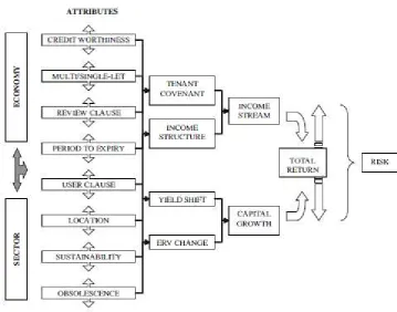
Figure 1. Real estate attributes, return and risk
Source: Jackson and Orr (2011)
Estimates of the Risk Premium
The level of the aggregate RP has been the subject of both empirical analysis and surveys of
investors. Blundell (2009) considers the RP at the national level in the UK and that it will reflect a
range of factors, such as illiquidity, expected earnings growth, default probability and so on. He
estimated the risk premium on real estate over the period 1981-2008 as 3.1%. Using the equation (k = RFR + RP g + d) which becomes (RP = k RFR + g d), his estimate includes the risk-free rate (as measured by the gross redemption yield on government bonds over the period) at 7.3% (RFR), 6.4% for the real estate initial yield (cap rate k), 6.3% for rental growth (g) and 2.3% for depreciation (d).. Previous empirical estimates of RP in the UK vary to include figures around 2% (Fraser, 1993, for
prime real estate); 3% (Hoesli and MacGregor, 2000); an average of around 4% in the pre-crash
period of 2002-06 (DTZ, annual); and at around a minimum of 3.5% in the post-crash period since
2008 (IPF/AREF, quarterly).1 Hutchison et al. (2012) attempt to advance B by modelling commercial risk premia within a time varying framework, reflecting market dynamics and cyclicality
in returns. Their Markov regime switching model suggests that regime shifts are less important in the
real estate market than in other investment and commodity markets. They found no evidence of
structural breaks in office risk premia, unlike other sectors, although warn that the aggregation of
data may be masking structural changes, implying the need to examine risk premia at a more
disaggregated level.
Growth and Depreciation
The final element of the Gordon pricing model set out in Equation 1 explicitly shows adjustments to
the cap rate to reflect expected future growth, further influenced by real estate depreciation.
Factors underpinning growth may be seen across the risk scale, such as the impact of the economy
on the real estate market overall and variation in this across sectors and submarkets. Likewise,
Crosby et al. UK
depreciation rates are also affected by factors across the risk scale; i.e. economic and local property
market factors as well as specific property attributes. There are two possible approaches to growth
expectations and depreciation. The first is to attempt to identify explicit variables for the
measurement of each of these components, however in this paper we adopt a different approach
and have wrapped them into the risk premium estimation, as set out below.
Most previous work does not disaggregate the components of the cap rate to the level of addressing
the measurement of growth and/or depreciation across the risk scale H J O
(2011) conceptual model set out in Figure 1 traces the causes of variation in returns at the stock level
back to the underlying attributes. This is important here it is proposed that growth and
depreciation expectations at the stock level are a function of the stock attributes and measurement
of these attributes therefore reflects investor expectations and, therefore, pricing.
Refining the real estate pricing model
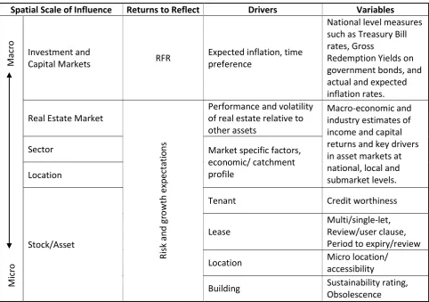
Table 1 provides a summary and conceptualisation of these complexities within a real estate pricing
model. Crucially, it attempts to locate the distinct elements along a risk scale, showing a
disaggregation of the components of the cap rate and causes of risk at distinct spatial scales. The
Table 1. The cap rate and risk scale
Spatial Scale of Influence Returns to Reflect Drivers Variables
M ac ro Investment and
Capital Markets RFR
Expected inflation, time preference
National level measures such as Treasury Bill rates, Gross
Redemption Yields on government bonds, and actual and expected inflation rates.
Real Estate Market
Ri sk an d g ro w th e xp e ctat io n s
Performance and volatility of real estate relative to other assets
Macro-economic and industry estimates of income and capital returns and key drivers in asset markets at national, local and submarket levels.
Sector Market specific factors,
economic/ catchment profile
Location
Stock/Asset
Tenant Credit worthiness
Lease
Multi/single-let, Review/user clause, Period to expiry/review
M
ic
ro Location
Micro location/ accessibility
Building Sustainability rating,
Obsolescence
This conceptu G
estate by identifying the different components of the risk premium. Thus, if RPREM is the part of the
risk premium for exposure to the real estate market and RPSTK is the part of the risk premium for the
stock/asset risk element attached to property-specific attributes, and, as above, if it is acknowledged
that elements of these attributes influence growth expectations and depreciation, then equation 1
can be modified into:
(2)
k = RFR + RPREM + RPSTK
RPREM and RPSTK can be refined further. Within RPREM, there are the three components of RPmkt (real
estate market risk), RPsct (real estate sector risk) and RPlocm (real estate market location risk). RPSTK is
the part of the risk premium for the stock/asset risk element attached to property-specific attributes.
This is composed of the four further elements of RPten (tenant risk), RPlse (leasing risk factors), RPlocs
(stock location risk) and RPbld (building risk). Each of these seven distinct components of the RP
derived from the various underlying market and stock-specific causes described above. Hence, this
gives:
(3)
k = RFR + (RPmkt + RPsct + RPlocm) + (RPten + RPlse + RPlocs + RPbld)
E G adapted and
extended by explicitly disaggregating the risk premium, following the conceptualisation set out in
Table 1.
3.
Operationalising the model
Previous studies
Few studies have sought to undertake empirical analysis at the level of disaggregation proposed by
equation (3), although some do offer important and useful findings. For instance, Sivitanidou and
Sivitanides (1999) estimated US local level (metropolitan) office cap rates using local-fixed and
time-variant components within a simple equilibrium adjustment framework, with time series/cross
sectional versions. These local and time variant variables were found to have greater explanatory
power for investors required returns and income growth expectations than national factors,
confirmed by Sivitanides et al. (2001) where fixed market characteristics create persistence differences in cap rates across markets, but national macro-economic forces account for some of the
variation.
Hendershott and MacGregor (2005) apply an error correction framework to appraisal cap rates in
prime UK locations and demonstrate that office and retail yields are inversely related to real
expected rental growth and positively related (but insignificantly) to real dividend growth. Dunse et al. (2007) examine the determination of initial yields in nine provincial office markets in the UK relative to the City of London. They use the basic pricing framework and error correction panel
model, with: the gross redemption yield on 15 year bonds to measure the nominal RFR; the RP is
captured by the dividend yield on the FTSE 100 (proxy for the return on alternative investments) and
the real value of financial institution transactions (
conditions); real rental growth (to proxy expected growth rates); with depreciation assumed to be
constant. A further two variables, following the work of Hendershott and MacGregor (2005), are
added to capture the deviations of rent and stock market dividend yield variables from the
Plazzi et al. (2008) and Plazzi et al. (2010) use transaction data for US Metropolitan Areas and build a set of simultaneous equations, derived from an extended Gordon framework, to examine the
cross-sectional dispersion of rental growth and expected returns (in their 2008 paper) and time variation in
expected returns, rental growth and cap rates at the area level (in their 2010 paper). They find that
cap rates cannot be used to forecast expected returns and call for further work on identifying the
determinants of real estate cap rates.
Current study
A framework for the estimation of the real estate pricing model developed here must recognise a
number of challenges. First, the causes of disparities in cap rates can be masked by a range of real
estate and transaction specific factors that operate across several spatial levels, and give rise to
spatial autocorrelation. Following Orford (1993) and Leishman (2009), who used multi-level analyses
when analysing local house prices to explicitly allow houses to be embedded within submarkets that
are influenced by local and higher spatial level factors, a similar nested hierarchy exists within the
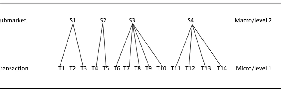
commercial real estate market. Figure 2 shows how investment transactions can conceptually be
represented as a simple two-level nested structure, where transactions are clustered within
submarkets and that there may be shared influences from particular submarkets on transactions
[image:11.595.76.543.468.617.2]within those submarkets.
Figure 2. A unit diagram for a two level nested hierarchy
Submarket S1 S2 S3 S4 Macro/level 2
Transaction T1 T2 T3 T4 T5 T6 T7 T8 T9 T10 T11 T12 T13 T14 Micro/level 1
A multi-level framework, similar to the approach taken by Sivitanidou and Sivitanides (1999), will
allow an exploration of the spatial variations in cap rates that are driven by submarket effects, while
also measuring the variation generated by the characteristics of the real estate, its tenants, its
purchaser and how wider macro-economic factors influence the expectations of purchasers with
regards to individual investments. This modelling framework is suitable here as it explicitly captures
within submarkets. Other statistical techniques, such as multiple regression, that ignore the effects
of clustering, give biased standard errors which can result in random variation being mistaken for
real effects.
Initially, a micro-level modelling framework is specified to capture the explanatory elements of,
firstly, the impact of attributes specific to the transacted real estate in the determination of real
estate cap rates achieved in each investment transaction and, second, as begun to be acknowledged
in the literature above, the wider contextual and behavioural factors that can affect the outcome of
the pricing decision, referred to here simply as transaction characteristics. This gives the level 1
Equation:
(4)
ij STK lj i
j
ij
RFR
RP
e
k
lij
0
0
where kij is the cap rate achieved in transaction i nested in submarket j and eij represents the
variation in yields that cannot be explained by the real estate and transaction characteristics. This is
extended from a regression model where
0j accommodates the possibility of j intercepts as thesecan vary across submarkets. The risk-free rate and its parameter, and the explanatory variables and
parameters, are represented by RFR,
i0,ij l
STK
RP and
lj, respectively. In theory there could be anynumber of explanatory variables within the underlying categories, but is used to
give a concise expression for the sum of the variables that determine the cap rate in transaction i
nested in submarket j and l represents the index of summation. These explanatory variables capture the specific real estate asset and transaction characteristics expected to impact on the return a
buyer expects on a transaction, whereas the risk-free rate is expected to influence all transactions in
much the same way regardless of submarket. An assumption underpinning this is that the residual
term (eij) follows a normal distribution with variance equal to
2 e
.With reference to the conceptual framework in Table
performance of investments over the holding period are a function of macro/micro factors,
beginning with conditions in the national capital markets and moving to real estate markets, to
include market, sector and location factors which, taken together, are referred to here collectively as
submarkets. Level 2 specifically captures the clustering of transactions within such submarkets, and
the influence of the structural traits of the submarket (such as size, composition and quality of the
transactions in the same submarket so it is necessary to add an area-level error term that allows for
variation between areas. Equation 5 allows for this by taking the intercept of Equation 4 (
0j) andspecifying it as:
(5)
j lj REM l
j 00 1
RP
00
This represents the macro-level equation. This equation assumes
around an overall average cap rate (
00) when all the predictors (lj
REM
RP
) are equal to zero.
RPREM captures the submarket-level explanatory variables and
0j represents the deviation of submarket j from this average. This is also termed the submarket-specific effect. The combination of Equations 4 and 5 forms a simple two-level hierarchical framework that recognises thedetermination of cap rates as a transaction process nested within submarkets:
(6) ij STK lj i j REM l
ij RP RFR RP e
k
lij
lj
00
1
0
0
This is a type of multi-level framework and allows for two sources of random variation,
at level 1 of the transaction process (eij) and at level 2 of submarkets (
0j). In keeping with analysisof variance models, the two variance components (var
eij
e2 and var
0j
u2) need to beestimated along with the other parameters. The total variance is
e2
2 and the proportion of thetotal variance attributed to submarkets can be estimated as
2/
e2
2
whereas theproperty-specific variance can be estimated as 1-
2/
e2
2
. The clustering of transactions intosubmarkets induces a correlation between the cap rates of pairs of transactions
( 2
'
cov
j i ij er er R
R ) which are located within the same submarket and the size of this correlation,
also referred to as the variance partitioning coefficient, should be the same as
2/
e2
2
. Inordinary least square regression there should be zero correlations between the residual terms.
In Equation 6, submarket variation in cap rates is allowed for by the inclusion of fixed effects in the
theoretical linear framework. This can be conceptualised as a series of submarket curves, each
having different intercepts for each submarket but being similar in slope due to the same micro-level
drivers having the same effects on the transaction process across all submarkets. However, it is
submarkets, and Bailey et al. (2012) highlight the benefit of the hierarchical approach in that it allows for the existence of more complex patterns of variance to be investigated. This can be
achieved by specifying an additional macro-level equation as:
(7)
nj n
nj
0
Equation 7 now allows for variation in the slopes of the submarket curves where the common slope
nj
is replaced by another random effect. From this a random-intercept and random-slope model,including level-2 variables and cross-level interactions, is derived by substituting Equation 7 into 6 to
give Equation 8.
(8) ij STK nj j STK j n l i STK n lj REM l
ij
RP
RP
RFR
RP
RP
e
k
ij n ij n lnij
1 ) ( 0 ) ( 0 0 100
This is our theoretical mixed effect framework for operationalising our model of real estate cap
rates. Within it,
ij n l
nij i l n j STK
STK n lj REM
l1
RP
0RP
0RFR
( )RP
( )00
representsfixed effects and j nj
RP
STKe
ijij
n
1
0
represents random effects which have two random effectsat the submarket level. I are
estimated and examined to see how effective the inclusion of the fixed and random effects is in
explaining cap rates.
4.
Data
An exploratory estimation of the framework set out above, to operationalise the real estate pricing
model, is undertaken using observed transactions in the global financial office market in central
London. The analysis explores a dataset of 497 transactions in the central London office market over
the period 2010 Q2-2012 Q3, representing every reported investment sale, after data cleaning and
checking.2 The data for the project are primarily provided by CoStar and comprise information on
individual transactions relating to the characteristics of the occupation, leases, buildings and
ownership. The building quality data from CoStar represent the first opportunity to fully explore the
pricing of real estate attributes in the UK and that has driven the timescale of the analysis. The
2
It is worth noting that this is significantly before the 2016 UK Referendum on EU membership was mooted in
dataset is the most comprehensive available, but it has its limitations. Additional data were collated
from CoStar, other sources such as EGi and provided by CBRE to both confirm and supplement the
individual real estate data from CoStar. There are a number of observations that are available from
multiple sources, for instance floorspace, and there were some discrepancies between sources.
Prolonged and systematic data checking and validation was undertaken.
In terms of the dependent variable, the CoStar dataset only provides initial yields3 for each
transaction, necessitating calculation of the equivalent yield4 required for the study. The equivalent
yield is the preferred measure in the UK context as it takes into account not only the level of the
initial rent, but also the reversion to a market rent (assuming current market levels) and the
scheduled date for this change in income stream (i.e. at review or lease expiry). It is common in the
UK that there are 5 years between changes in rental levels due to periodic review clauses in the lease
and the lack of indexation between these periodic revisions. Thus, equivalent yields more fully reflect
the level of cap rates in the UK market and are therefore the primary measure used within UK
valuation and performance measurement systems (see, for example, Baum and Crosby, 2008). Figure
3 indicates the discrepancies between the two measures of initial and equivalent yield. It illustrates
the London City and West End office markets between 1981 and 2015 and shows that, in the West
End, apart from one year in the early 1990s when they were the same, equivalent yields were higher
than initial yields, indicating positive reversionary potential (rent passing is lower than market rent).
The data for the City office market illustrate that the post 1990 downturn created a period of
over-renting (rent passing is higher than market rent) for four years. The main two reasons for equivalent
yields being higher than initial yields for most of the period is that, normally, passing rents lag
market rents and vacancies are not assumed to be infinite in the equivalent yield calculations.
3
CoStar actually reports net initial yield which is purely the rent passing divided by the transaction price plus
. Vacancies are therefore ignored causing properties with high vacancies to have low
initial yields.
4
Figure 3: Initial and Equivalent Yields, London West End and London City Offices 1981 to 2014
Source: IPD Annual UK Property Index (MSCI)
Estimation of the equivalent yield requires some additional data, these being the market rent and
the unexpired term to the next rent change.
Market rents have been determined by comparison to new lettings within the same building. Where
these lettings are not contemporaneous with the transaction date, they have been updated using
data from the CBRE Rent and Yield Monitor (CBRE, quarterly). The actual rent point valuations
through time were given to the project confidentially and these were matched with the individual
transactions within the transaction database.
The period to the next rent change was identified from the lease data collected for each transaction
at the transaction date. Where a property was multi-tenanted, a weighted (by rent) average
unexpired term was used. Not all lease expiry and rent revision dates were known for all leases
within a transaction. Where they were not known across all leases in a property, a default of 2.42
years was used, being the average across the entire sample for those transactions where the next
rent change was known.
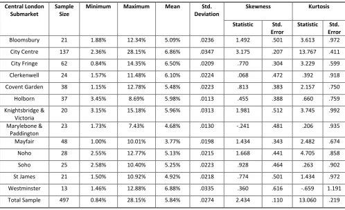
Table 2 presents the summary descriptive statistics for the estimated cap rates in the form of
equivalent yields over 13 contiguous submarkets as defined by market agents (those with very small
sample sizes are merged into the neighbouring, most relevant, submarket). The skewness and
with the normal distribution assumption and require transformation, using natural logarithms, to
[image:17.595.66.565.169.473.2]give a normal distribution for this, the dependent variable.
Table 2. Descriptive statistics forequivalent yields imputed for the sample of transactions across
submarkets
Central London Submarket
Sample Size
Minimum Maximum Mean Std. Deviation
Skewness Kurtosis
Statistic Std. Error
Statistic Std. Error
Bloomsbury 21 1.88% 12.34% 5.09% .0236 1.492 .501 3.613 .972
City Centre 137 2.36% 28.15% 6.86% .0347 3.175 .207 13.767 .411
City Fringe 62 0.84% 14.35% 6.50% .0209 .770 .304 3.229 .599
Clerkenwell 24 1.57% 11.48% 6.10% .0224 .068 .472 .392 .918
Covent Garden 38 1.15% 12.78% 5.48% .0223 .813 .383 2.157 .750
Holborn 37 3.45% 8.69% 5.98% .0113 .455 .388 .660 .759
Knightsbridge & Victoria
20 3.15% 15.18% 5.96% .0313 1.981 .512 3.745 .992
Marylebone & Paddington
23 1.73% 7.43% 4.68% .0130 -.241 .481 .206 .935
Mayfair 48 1.00% 10.01% 3.77% .0198 1.434 .343 2.482 .674
Noho 28 2.55% 12.77% 5.13% .0215 1.668 .441 4.705 .858
Soho 25 2.58% 10.40% 5.25% .0223 .928 .464 .263 .902
St James 21 1.50% 10.92% 4.92% .0218 .774 .501 1.434 .972
Westminster 13 1.46% 12.88% 6.88% .0335 .360 .616 -.659 1.191
Total Sample 497 0.84% 28.15% 5.84% .0274 2.434 .110 13.060 .219
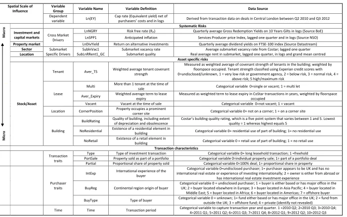
The independent variables included in the analysis are largely derived from the literature, set out
above. They are summarised in Table 3 and can be seen to follow the extended pricing model in
equation (3) with the addition of variables to enable segmentation of the results for transaction
characteristics, being the wider contextual and behavioural differences in transaction type,
purchaser characteristics and time period. Two areas require expansion. Firstly, at the market level,
the two components of real estate sector and location are, in effect, office submarkets, given the
focus of the study on central London office markets. Thus, they are measured together using vacancy
and rental variables to proxy the relative quality of each submarket, encapsulating additional factors
identified as important, such as local economic structure and catchment. While the lagged vacancy
data are straight-forward in their representation of perceptions of submarket quality, the differential
rental measure used to indicate market quality is constructed from lagged rents, adjusted for
inflation through the time frame of the project and centring around the average rent (grand mean)
across all the submarkets included in the study. This allows us to interpret changes in this variable as
Table 3. Exploring the determinants of office cap rates: variables and data
Spatial Scale of Influence
Variable
Group Variable Name Variable Definition Data Source
Dependent
variable Ln(EY)
Cap rate (Equivalent yield) net of
Derived from transaction data on deals in Central London between Q2 2010 and Q3 2012
M
a
cr
o Systematic Risks
Investment and
capital markets Cross Market
Drivers
LnNGRY Risk free rate (Rrf) Quarterly average Gross Redemption Yields on 10 Years Gilts in logs (Source BoE) LnSPP1 Anticipated inflation Services Producer price Index, lagged one quarter and in logs (Source NSO)
Property market LnDivYield Return on alternative investments Quarterly average dividend yields on FTSE-100 index (Source Datastream)
Sector Submarket Specific Drivers
SublnVac1 SubLnRRent1_GC
Submarket vacancy rate Submarket quality
Average submarket vacancy rate from Costar; lagged one quarter Real average rent in submarket, lagged one quarter, in logs and grand mean centred
Location
Asset specific risks
Stock/Asset
Tenant Aver_TS Weighted average tenant covenant strength
Measured as weighted average of covenant strength of tenants in the building; weighted by floorspace occupied. Tenant strength classified using Experian credit scores with 0=undisclosed/unknown, 1 = very low risk or government agency, 2 = below risk, 3 = normal risk, 4 =
above risk; 5 high/maximum risk
Lease
Multi More than 1 tenant at the time of
sale Categorical variable 0=single or vacant; 1 = multi let
Aver_Expiry Weighted average term to lease expiry
Measured as weighted term to lease expiry in CoStar transactions in years, weighted by floorspace occupied
Vacant Vacant at the time of sale Categorical variable 0=not vacant; 1 = vacant
Location CornerPosition Property occupies a prominent
corner site Categorical variable 0= not on a corner; 1 = on a corner site
Building
BuildRating Quality of building, including extent of depreciation and obsolescence
C L
quality = 1 whereas highest equals 5
M
ic
ro NoResidential
Existence of a residential element in
building Categorical variable 0= residential use of part of building; 1= no residential use
NoRetail Existence of a retail element in
building Categorical variable 0 = retail use of part of building; 1 = no retail use
Transaction characteristics
Transaction traits
Type Type of investment transaction Categorical variable 0= long leasehold transaction; 1 =freehold PortSale Property sold as part of a portfolio Categorical variable 0=individual property sale; 1= part of a portfolio deal
Partial Proportional share of property sold Categorical variable 0=100% deal; 1= proportional share in property
Purchaser traits
IntExp International experience of the buyer
Categorical variable 0=undisclosed purchaser; 1= purchaser appears to be UK and has no international real estate or experience of investing internationally; 2 = owner is either from abroad or
has international real estate investment experience
BuyReg Continental region origin of buyer
Categorical variable 0 = undisclosed purchaser; 1 = buyer is either based or has major office in the UK; 2 = buyer located elsewhere in Europe; 3 = buyer located in Asia Pacific; 4 = buyer located in
Middle East; 5 = buyer located in Africa; 6 = buyer located in Americas; 7 = offshore buyer
BuyType Type of buyer Categorical variable 0 = unknown; 1= fund either based or has major office in the UK; 2 = fund from outside the UK; 3 = offshore fund; 4 = private (identify not revealed)
Secondly, following the derivation of the pricing model, the disaggregation of the RP into its
component parts traces expectations of growth and depreciation to underlying causes at both
market and stock levels. In terms of data requirements and modelling approaches, this represents
advancement on previous studies that have struggled to find appropriate measures for growth
and/or depreciation which have, in some instances, been ignored or assumed away as constants.
Here, expected depreciation at the stock/asset level, is a function of location and building
[image:19.595.67.534.246.633.2]characteristics, captured by C “ measure of building quality, set out in detail in Table 4.
Table 4. CoStar building classification for offices
Building
Rating Definition
Percentage in Sample
1 Star A very poor quality building with no tenant and little prospect of attracting a tenant because it is in very poor condition with substantial physical and structural defects and does not offer viable accommodation.
0.0%
2 Star An older building, typically more than 20 years old, with the majority of the accommodation cellular. Poor quality reception areas with no lifts or old, poorly maintained lifts and generally poor maintenance with physical or structural defects. Rents will be substantially lower than for 3 Star buildings and close to the lowest levels achieved locally.
1.2%
3 Star This is an older building that offers basic open plan accommodation and has been partly renovated but the interior has not been completely refurbished. Plant and other servicing likely to be outdated and inferior with some functional limitations although still reasonably well maintained.
39.2%
4 Star A modern building, completed or renovated in the last 10 years, which offers good quality modern open plan space which is well maintained and managed. Externally less architecturally impressive than a 5 Star building. Offers good quality open plan office accommodation with raised floors, some form of air cooling system and adequate passenger lifts but is of a more basic design than a five star building.
47.6%
5 Star A landmark building, either new built or extensively renovated within the last 5 years; to provide top specification accommodation and typically have a BREEAM rating of VERY GOOD, EXCELLENT or OUTSTANDING. If the building is older then the interior will be completely reconstructed with only the historical façade or structural frame remaining, and maintained and managed to the highest standard. Commands rents at or close to the top achievable rents in the local market.
12.0%
Source: CoStar (2013)
The CoStar building quality rating is a single categorical variable that measures the condition of the
building through a grading of its specification, quality of maintenance, architectural quality, energy
performance and prominence of its location. The building quality data are a new initiative and the
ratings are collected by observation. Observers are given a set of criteria in order to grade each
refurbishment/redevelopment opportunities and were excluded from the investment transaction
dataset leaving the bulk of properties in grades 3, 4 and, to a lesser extent, grade 5.
5.
Findings
Each stage of the model development is operationalised and the estimations, using a Restricted
Maximum Likelihood (REML) method5, are given in Tables 5 and 6. The analysis begins by testing
Equation 6, the basic two-level framework. This is the same as
k
ij
00
0j
e
ij where theexplanatory variables and parameters (represented by
i 0RFR,
lj
REM l1
RP
and
lij
STK
ljRP
) areomitted, leaving the intercept (
00) in the empty model (shown in Table 5 as Estimation 1) torepresent the overall average cap rate. It is shown in natural logs (-2.9800) to create a normal,
non-skewed data series and, when transformed back into percentage, gives an average cap rate of
5.08%.6 Starting at this point in the analysis is useful as it allows us to then explore how cap rates
differ due to submarket effects, stock-specific effects and transaction characteristics.
The intra-submarket correlation for the sample over the study period captures a significant
proportion (85.45%) of the variation in cap rates around the estimated mean.7 This conforms with a priori expectations, as previous studies show that specific risks contribute a large proportion of the investment risk attached to an asset and that default and void risks are primarily driven by the
characteristics of the tenants, lease terms and property, as set out in the model by Jackson and Orr
(2011).
It is noteworthy that the variance between transactions is 5.9 times larger than the variance
between submarkets (see estimate of covariance parameters near bottom of Table 5). However, a
not-insignificant 14.56%8 of the differences in cap rates in the sample can be traced to submarket
differences. Thus, both stock and submarket variables need to be investigated to fully explain cap
rates. The relatively small size of the submarket-specific influence may surprise some analysts, but
5
REML is one of two possible estimation techniques employed in most multi-level programs and selects the
model parameter values that maximise the likelihood function that is calculated from a set of data that has been transformed to focus on the parameters of interest. This transformation is achieved by removing the effect of the fixed variables.
6 This average is the common average across all the submarkets allowing for between and within submarket
variation and the bias generated by between submarket variations.
7
This is estimated as 1-(0.0285/(0.0285+0.1672)).
this could reflect the fact that many buyers are overseas and are seeking to buy in London as a
perceived politically and financially stable international market, rather than very specific parts of
London. Given the gap between cap rates in London and the rest of the UK (CBRE, quarterly), this
London effect would be expected to be more noticeable if submarkets outside London had been
included. The impact of overseas purchasers on cap rates is one of the factors tested subsequently.
Table 5. Results of empty multi-level models
Fixed Effects Estimation 1 Estimation 2 Estimation 3 Estimation 4 Estimation 5
Intercept -2.9800 *** -2.9801 *** -2.9026 *** -2.9556 *** -2.9801 ***
SublnRRent1_GC (Submarket quality) -.3159 * -.4638 ** -0.5465 *** -0.3159 *
Time = 2010 Q2 -.0935
Time = 2010 Q3 -.1189
Time = 2010 Q4 -.0658
Time = 2011 Q1 -.1005
Time = 2011 Q2 -.1567 **
Time = 2011 Q3 -.1643 **
Time = 2011 Q4 -.0122
Time = 2012 Q1 .0451
Time = 2012 Q2 -.0901
Estimates of Covariance Parameters
Residual .1672 *** .1680 *** .1676 *** 0.1723 *** 0.1680 ***
Intercept [subject = Submarket_id]
Variance .0285 ** .0181 * .0158 *
0.0181 *
TIME [subject = Submarket_id]
Variance 0.0143 ** 0.0000
Model Fit Statistics
-2 Restricted Log Likelihood 548.73 547.72 568.20 575.88 547.72
Akaike's Information Criterion (AIC) 552.73 551.72 572.20 579.88 553.72
Hurvich and Tsai's Criterion (AICC) 552.75 551.74 572.23 579.90 553.77
Bozdogan's Criterion (CAIC) 563.14 562.13 582.57 590.29 569.33
Schwarz's Bayesian Criterion (BIC) 561.14 560.13 580.57 588.29 566.33
*** significance at the 1% confidence level; ** at the 5% confidence level; * at the 10% confidence level.
The next stage of the analysis explores the influence of adding submarket variables as fixed effects to
give Estimation 2. Here, we add the level-2 submarket variable SublnRRent1_GC to capture market
quality. This mean-centred variable measures the change in the difference between average rental
the average cap rate across all submarket locations remains at 5.08% (transformed from -2.9801 in
natural logs), there is a clear improvement in explanatory power. Estimation 2 indicates that
investors purchase at lower cap rates for better submarket quality: for every 1% the submarket
location rental value rises above the change in average Central London rental value, the cap rate falls
by 0.36% (transformed from 0.3159).9 This is statistically significant and, thus, the unexplained
variance between submarkets falls by 36.49%. The reduction in the Akaike's Information Criterion
(AIC); Hurvich and Tsai's Criterion (AICC); Bozdogan's Criterion (CAIC) and Schwarz's Bayesian
Criterion (BIC) also suggest an improvement in fit.10 However, this improvement in fit is still relatively
small with the Wald Z statistic testing11 of the variance components in the covariance parameters
suggesting that unexplained transaction variation still exists at the 1% confidence level. Although
such tests can be unreliable (Snijders and Bosker, 1994), the fall in the Wald Z statistics to 1.786 for
the unexplained submarket variation suggests (but only at the 10% confidence level) that a little
variation exists between submarkets and the inclusion of the level 2 predictor does not remove all
the submarket specific variation present in cap rates.12
The first of the wider contextual transaction characteristics is introduced in Estimation 3, where
movements in the level of cap rates associated with the timing of the transaction are tested.13 With
only two exceptions (Q2 and Q3 in 2011) there are no significant differences over the study period,
possibly implying that yield movements were static over the period of analysis. Market evidence
supports this finding, with CBRE (various) indicating that prime yields in central London offices
remained largely static for most of this analysis period. Statistically, the addition of the time variables
fails to improve fit. When retested with time specified as random effects (Estimation 4) this results in
higher information criterion statistics, suggesting the fit has been negatively affected by the inclusion
9 For example, if the rent in a submarket is £20 per square foot above the average central London rental
value and that difference grows by 10% to £22, assuming all else remains unchanged, the cap rate will fall by 3.6%; i.e. from 5.08% to 4.9%.
10 Selection between alternative non-nested multi-level models can be made using goodness of fit statistics
that are relative estimates of the information lost when a given model is used on a given set of data. The AIC, AICC, CAIC and BIC are variants of a goodness of fit test that use a likelihood function with either a penalty for the number of estimation parameters included in the model (AIC and BIC) or sample size (AICC and CAIC). The model with the lowest AIC, AICC, CAIC and BIC are preferred (Bozdogan, 2000).
11 The Wald test is a parametric statistical test that in this instance is used to test the significance of the null
hypothesis that the difference between the estimated sample variance and the true variance is equal to zero. If the test rejects the null hypothesis then a statistical difference exists and this is assumed to be due to the model and its variance not capturing the true variance. The level of confidence in rejecting the null hypothesis is denoted by ***for the 1% confidence level; ** for the 5% confidence level and * for the 10% confidence level.
12 The influence of other submarket measures (absolute and grand mean centred submarket vacancy rates
and actual rental growth, adjusted for inflation) in explaining cap rates were examined. None of these results are reported in the paper as they were insignificant and failed to improve explanatory power.
of a time random effect. Time, at least during this period of study, does not help explain the
variation in cap rates.14,15
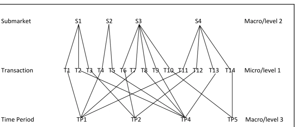
Estimation 5, the last in Table 5, checks for the possibility for time to be a third level of spatial
influence where it affects multiple transactions over more than one submarket (as illustrated in
Figure 4). This can be captured as a non-nested third level estimation. The level 2 and 3 random
effects in Estimation 5 have been included as single identities.16 A comparison of AIC and BIC
statistics implies that the simpler 2 level hierarchical frameworks are a more relevant structure to
[image:23.595.69.551.286.494.2]adopt.
Figure 4. A unit diagram for a two level nested hierarchy and non-nested third level
Submarket S1 S2 S3 S4 Macro/level 2
Transaction T1 T2 T3 T4 T5 T6 T7 T8 T9 T10 T11 T12 T13 T14 Micro/level 1
Time Period TP1 TP2 TP4 TP5 Macro/level 3
Table 6 presents the analysis when variables measuring the RFR rate are introduced, as are
additional components of the RP, alongside the remaining wider contextual and behavioural factors
relating to transaction characteristics, the latter as (level 1) explanatory variables. As detailed in
Table 3, the variables run through the risk scale, starting at the macro end with the RFR
14 One concern was that there is not a sufficient number of observations in each time period across 13
submarkets; this was therefore reviewed across alternative submarket definitions (first the three City, West End and Mid-Town submarkets and, second, the merging of contiguous submarkets into seven groupings down from the original 13). In each of these iterations the time fixed effects and random effects remained insignificant, while the variation between submarkets became blurred and insignificant. The results are not, therefore, reported here.
15
Other random effects, tested in our mixed effects estimations as random slope effects, were absolute and grand mean centred submarket vacancy rates and actual rental growth, adjusted for inflation and grand centred submarket rents, adjusted for inflation. The addition of these variables as random effects did not improve explanatory power. The results are not reported in this paper.
16
expectation regarding the risk free rate of return and anticipated inflation; and, moving along the
scale to the RP with additional real estate market factors, to include return on alternative
investments; and, at the micro end of the risk scale: variables capturing the tenant, lease, location
and building specific attributes of the asset. The rate of return expected on a risk free asset, the
weighted average term to expiry and the
measured as continuous variables, with the remaining attributes captured through categorical
variables. The intercept is removed to allow differentiation between the mean cap rate by type of
transaction, with 0 denoting the purchase of a long leasehold and 1 representing a freehold.
Estimation 6 presents a detailed fixed effects model which contains possible predictors, as listed in
Table 3, in an attempt to assess which individual variables contribute to London office cap rates but
not all are significant. The majority of the properties in the sample are homogeneous in that they are
occupied (Vacant=0), sold individually (PortSale=0) and sold as complete units (Partial=0), therefore
these dichotomous variables are not significant in explaining differences in cap rates over and above
the base model. In addition, the unit being on a corner site (CornerPosition=0) is also insignificant
and, along with insignificant variables at the macro end of the scale that gauge anticipated inflation
and dividend yields on shares as an alternative form of investment, these variables are removed in
Estimation 7. This represents a more parsimonious fixed effects estimation17 which yields lower AIC
and BIC statistics and nearly all the fixed effects are significant at the 90% confidence level. The
A T“
(Aver_Expiry), some CoStar building quality ratings (BuildRating), and the category for international
experience that represents when this buyer information is unknown (IntExp=0). This estimation of
the model specifies that the average cap rates for long leaseholds and freeholds based on a sample
of the transactions where the buildings being transacted are rated as 5 star, top quality stock and
bought by buyers with international experience are 3.52% (transformed from -3.3454) and 3.25%
(exponent of -3.4254), respectively.
17
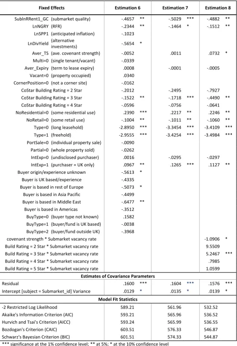
Table 6. Results of multi-level models containing property, buyer and transaction variables
Fixed Effects Estimation 6 Estimation 7 Estimation 8
SublnRRent1_GC (submarket quality) -.4657 ** -.5029 *** -.4882 **
LnNGRY (RFR) -.2344 ** -.1464 * -.1512 **
LnSPP1 (anticipated inflation) -.1023
LnDivYield (alternative
investments) -.5654 *
Aver_TS (ave. covenant strength) -.0052 .0011 .0732 *
Multi=0 (single tenant/vacant) -.0339
Aver_Expiry (term to lease expiry) .0008 -.0001 -.0005
Vacant=0 (property occupied) .0340
CornerPosition=0 (not a corner site) -.0162
CoStar Building Rating = 2 Star -.2012 -.2495 -.7927
CoStar Building Rating = 3 Star -.1522 ** -.1718 *** -.4490 **
CoStar Building Rating = 4 Star -.0596 -.0756 -.0641
NoResidential=0 (some residential use) .2390 *** .2217 ** .2246 **
NoRetail=0 (some retail use) -.1004 ** -.1011 ** -.1060 **
Type=0 (long leasehold) -2.8950 *** -3.3454 *** -3.4109 ***
Type=1 (freehold) -2.9555 *** -3.4254 *** -3.4984 ***
PortSale=0 (individual property sale) -.0090
Partial=0 (whole property sold) -.0262
IntExp=0 (undisclosed purchaser) .0016 -.0295 -.0297
IntExp=1 (purchaser = UK only) .0967 ** .1265 *** .1127 **
Buyer origin/experience unknown -.5613 *
Buyer is UK based/experience -.4335
Buyer is based in rest of Europe -.5073 *
Buyer is based in Asia Pacific -.4499
Buyer is based in Middle East -.6477 **
Buyer is based in Americas -.3512
BuyType=0 (buyer type not known) .1582
BuyType=1 (buyer/fund is UK based) -.0038
BuyType=2 (buyer/fund outside UK) -.3968
covenant strength * Submarket vacancy rate -1.0906 *
Build Rating = 2 Star * Submarket vacancy rate 9.5509
Build Rating = 3 Star * Submarket vacancy rate 5.2467 ***
Build Rating = 4 Star * Submarket vacancy rate .7985
Build Rating = 5 Star * Submarket vacancy rate 1.0599
Estimates of Covariance Parameters
Residual .1600 *** .1604 *** .1576 ***
Intercept [subject = Submarket_id] Variance .0129 * .0135 * .0139 *
Model Fit Statistics
-2 Restricted Log Likelihood 589.21 561.96 532.52
Akaike's Information Criterion (AIC) 593.21 565.96 536.52
Hurvich and Tsai's Criterion (AICC) 593.24 565.99 536.55
Bozdogan's Criterion (CAIC) 603.51 576.33 546.87
Schwarz's Bayesian Criterion (BIC) 601.51 574.33 544.87
At the macro end of the risk scale, Estimation 7 shows that the fixed effect for contemporaneous
nominal risk free rates suggests that falling Gross Redemption Yields raise capitalisation rates. This is
the same result even when lagged rates or alternative measures such as the Treasury Bill rate are
used. Either real estate investors are slow to react to changes in the capital markets, as noted in the
literature, or falling bond yields encourage investors to shift away from assets with the highest
implied growth rates, especially if falling bond yields are a product of expected decreases in inflation
that may impact on equity income flows.18 Moving along the risk scale, Estimation 7 shows that
mixed use within real estate assets impacts on cap rates. Where there is a residential component in
the building, it seems that investors are pricing this as a risk and raising cap rates. In contrast, where
offices have a retail component, this is perceived to lower risk and therefore lower cap rates.
The level of international experience of the buyer is also significant, with the results indicting that
investors with international experience appear to buy at lower cap rates and, thus, higher prices,
than home investors with no international experience.The origin of buyers has been removed from
Estimation 7 as the inclusion of this variable failed to improve fit and multicollinearity appeared to
exist between this variable and the definition used to categorise the international investment
experience of buyers. Yet, when included, the results (see back to Estimation 6) confirm the finding
cap rates, suggesting that buyers from the Middle
East and Europe transacted at lower cap rates than other regional buyers.
Estimation 8 specifies cross-level interactions to capture the possibility that our submarket measure
of market quality may be linked to the quality of buildings. It also allows for the influence of historic
by lease expiry terms. The results show a base cap rate of 3.30% for investors with experience in
international markets buying long leaseholds with no retail or residential component in a top quality
building (transformed from -3.4109). For a comparable freehold, the base cap rate is 3.02%
(transformed from -3.4984). Key changes in the results given by Equation 8 include that the effect of
tenant covenant strength now has a significant role in explaining cap rates, with rates increasing with
increased covenant risk. The effect of building quality in explaining the differences in cap rates is
inconclusive (even contradictory to expectations) although the positive and significant cross
18
interaction figures suggest that, in times of higher vacancy rates, cap rates are higher for buildings of
poorer 3 star ratings than for buildings with higher ratings.
The significant variables driving transaction cap rates (in logs) are the risk free rate, type of real
estate interest, existence of retail and residential space in the building, and
strength. Investment experience also has a significant influence, with experience in only UK markets
resulting in upwards shifts in cap rates of 0.36% for freeholds and 0.39% for long leaseholds. The
lower AIC and BIC tests suggest Estimation 8 is the better model, which is also confirmed by a
Likelihood Ratio Test which describes the difference in deviance between Estimation 7 and 8,
Estimations 1 and 8, and Estimations 2 and 8 and suggests Estimations 8 fits the data better.19
6.
Discussion and Conclusions
The purpose of this study is to examine the pricing of direct real estate, focusing on the
determination of cap rates and, more especially, the real estate attributes that determine the risk
premium. Through this, a refined pricing model for direct real estate is proposed, extending previous
understanding and reflecting the unique complexities of the asset and its context. Application of the
model is demonstrated through the development of a spatially robust multi-level framework and
subsequent estimation using observed cap rates for office properties in the central London global
office markets.
The analysis of cap rates, focusing on the disaggregation of the risk premium, is developed from an
analysis of the literature and uses the concept of a risk scale to identify the spatially distinct
component parts of the risk premium. This, then, underpins the revised pricing model which reveals
the complex components of the previously aggregated and opaque RP, with estimation of each
subsequently demonstrated. Further, the catch-all categories of growth and depreciation are traced
back to their causes, further enabling robust estimation and, importantly, avoiding potential
endogeneity issues with these latent variables.
Operationalisation of the model is presented here through a cross-sectional inter-temporal analysis
employing a dataset of real estate transactions in the central London office sector over a two and a
half year period. The dataset contains asset-specific information not previously released by CoStar
19