This is a repository copy of
Forcing-dependent dynamics and emergence of helicity in
rotating turbulence
.
White Rose Research Online URL for this paper:
http://eprints.whiterose.ac.uk/99700/
Version: Accepted Version
Article:
Dallas, V and Tobias, SM (2016) Forcing-dependent dynamics and emergence of helicity
in rotating turbulence. Journal of Fluid Mechanics, 798. pp. 682-695. ISSN 0022-1120
https://doi.org/10.1017/jfm.2016.341
[email protected] https://eprints.whiterose.ac.uk/ Reuse
Unless indicated otherwise, fulltext items are protected by copyright with all rights reserved. The copyright exception in section 29 of the Copyright, Designs and Patents Act 1988 allows the making of a single copy solely for the purpose of non-commercial research or private study within the limits of fair dealing. The publisher or other rights-holder may allow further reproduction and re-use of this version - refer to the White Rose Research Online record for this item. Where records identify the publisher as the copyright holder, users can verify any specific terms of use on the publisher’s website.
Takedown
If you consider content in White Rose Research Online to be in breach of UK law, please notify us by
Forcing-dependent dynamics and emergence
of helicity in rotating turbulence
Vassilios Dallas
†
and Steven M. Tobias
Department of Applied Mathematics, University of Leeds, Leeds LS2 9JT, UK
(Received ?; revised ?; accepted ?. - To be entered by editorial office)
The effects of large scale mechanical forcing on the dynamics of rotating turbulent flows are studied by means ofdirectnumerical simulations, varying systematically the nature of the mechanical force in time. We find that the statistically stationary solutions of these flows depend on the nature of the forcing mechanism. Rapidly enough rotating flows with a forcing that has a persistent direction relatively to the axis of rotation bifurcate from a non-helical state to a helical state despite the fact that the forcing is non-helical. We demonstrate that the nature of the mechanical force in time and the emergence of helicity have direct implications on the cascade dynamics of these flows, determining the anisotropy in the flow, the energy condensation at large scales and the power-law energy spectra that are consistent with previous findings and phenomenologies under strong and weak turbulence.
Key words:
1. Introduction
The effects of the Coriolis force on a turbulent fluid flow become important at suffi-ciently high rotation rates altering its dynamics (Tritton 1988). Experiments and simu-lations reveal that fast rotation renders the flow quasi-two-dimensional (quasi-2D), since fast rotation suppresses the velocity gradients along the axis of rotation as shown by the Taylor-Proudman theorem (Proudman 1916; Taylor 1917). Under such conditions, the flow sustains inertial waves whose frequency is proportional to the rotation rate (Lighthill 1965; Greenspan 1968).
The interplay between inertial waves and eddies in rotating fluids makes the problem of rotating turbulence very rich. Many experimental studies at a wide range of parameters have elucidated the dynamics of such flows (Hopfinger & Heijst 1993; Ruppert-Felsot et al. 2005; Davidson et al.2006; Bewley et al.2007; van Bokhoven et al. 2009; Moisy et al. 2011). Many numerical studies have also been carried out on rotating turbulence. The regime for which both the turbulence is fully developed (large Reynolds numbers) and the flow is fast rotating (small Rossby numbers) puts strong restrictions on the scale separation requirements in simulations. Therefore, most of the early numerical investigations were focused on decaying rotating turbulence (Bartelloet al.1994; Hossain 1994; Cambonet al.1997; Morinishiet al.2001; Teitelbaum & Mininni 2011; Yoshimatsu et al. 2011). More recent studies have been performed on forced rotating turbulence both at large (Yeung & Zhou 1998; Mininni & Pouquet 2010; Mininniet al.2012) and small scales; the latter to study the dynamics of the inverse cascade (Smithet al. 1996; Pouquet et al.2013; Deusebio et al.2014). The computational costs prevent in general
the exhaustive coverage of the parameters space with most numerical studies reaching either large Reynolds numbers and moderate Rossby numbers or moderate Reynolds numbers and small Rossby numbers. Note that these simulations, with the exception of a very recent study which reached steady states and covered extensively a fairly large portion of the parameters space (Alexakis 2015), have not reached statistically stationary solutions because very long integration times are required.
Although these studies were numerous and an adequate portion of the parameters space was covered there are still disparate results in different cases — for example, different power law spectra withE(k)∝k−5/3,k−2andk−5/2, supported theoretically by strong and weak-wave turbulence phenomenologies (Kolmogorov 1941; Zhou 1995; Galtier 2003; Pouquet & Mininni 2010). Moreover, a recent investigation showed sensitivity to forcing in that different results for the large scales of a flow that was forced at intermediate scales (Senet al.2012) when energy was injected exclusively to the quasi-2D component of the flow and when it was injected solely to the inertial waves. The injection of helicity into the flow has also shown alterations on the behaviour of the cascade (Pouquet & Mininni 2010). Forcing dependent dynamics have been observed in various other systems such as in two-dimensional (2D) turbulence (Bracco & McWilliams 2010; Boffetta & Ecke 2012), in beta-plane turbulence (Maltrud & Vallis 1991) and in magnetohydrodynamic turbulence (Dallas & Alexakis 2015).
The present work focuses on the effects of the mechanical force on the dynamics of rotating flows by means of numerical simulations, varying systematically the memory time scale of the mechanical force (i.e. the time scale of which the phases of the force are randomised). The behaviour of different mechanical forcing mechanisms on the flows is also considered for different rotation rates. To the best of the authors’ knowledge this is the first study of forced rotating flows in the steady state regime where the effects of a large scale external force on the dynamics are studied extensively.
The paper is structured as follows. All the necessary details of the formulation of our direct numerical simulations (DNS) of forced rotating turbulence are provided in Sec. 2. Section 3 analyses the dynamics of the flows with different memory time scales of the forcing mechanism for a given Rossby number. Here, we also focus on the spontaneous emergence of helicity in our flows and its influence on the anisotropy and on the spectral dynamics. In Sec. 4 we describe the Rossby number dependence on flows with different type of forcing mechanisms and we justify the spontaneous mirror-symmetry breaking in our flows even though net helicity is not injected directly. Finally, in Sec. 5, we conclude by summarising our findings and we discuss the implications of our work.
2. Numerical Simulations
In this study, we consider the three-dimensional (3D) incompressible Navier-Stokes equations in a rotating frame of reference
∂tu+ω×u+ 2Ω×u=−∇P+ν∇2u+f, (2.1)
where u is the velocity field, ω = ∇×u is the vorticity, P is the pressure, ν is the
kinematic viscosity, and f is an external mechanical force. In a Cartesian domain, we choose the rotation axis to be in thezdirection withΩ= Ωez, where Ω is the rotation
frequency. In the ideal case ofν= 0 andf = 0, Eq. (2.1) conserves the energyE=1 2h|u|
2i
τm/τN L 0.5 0.5 0.5 0.5 0.5 0.5 4.0 32.0 128.0 ∞ ∞ ∞ ∞ ∞ ∞ ∞
Rof 0.01 0.05 0.1 0.1 0.2 0.5 0.1 0.1 0.1 0.01 0.05 0.1 0.1 0.2 0.33 0.5
Ref 333 333 333 714 333 333 333 333 333 333 333 333 714 333 333 333 Ω 50.0 10.0 5.0 5.0 2.5 1.0 5.0 5.0 5.0 50.0 10.0 5.0 5.0 1.0 1.5 1.0
ν(×10−3) 3.0 3.0 3.0 1.4 3.0 3.0 3.0 3.0 3.0 3.0 3.0 3.0 1.4 3.0 3.0 3.0
N 256 256 256 512 256 256 256 256 256 256 256 256 512 256 256 256
Table 1: Numerical control parameters of the DNS.
The external mechanical forcing in Eq. (2.1) is given by
f =f0 X
kf
sin(kfy+φy) + sin(kfz+φz)
sin(kfx+φx) + sin(kfz+φz)
sin(kfx+φx) + sin(kfy+φy)
, (2.2)
where φx, φy, φz are phases, which are randomised every τm, the so called memory time scale, which is one of the control parameters in our study. The forcing is applied at wavenumber amplitudes|k|=kf = 2, 3 and 4, wherekfdenotes the forcing wavenumber. The random phases are specific to akf mode and the random change of phases is done instantaneously for all phases.In the limit ofτm→0 we have essentially a random delta
correlated in time forcing with the phases randomised at each time step, whereas when we choose τm =∞ we randomise the phases only att = 0 in the duration of the runs
and hence we apply a time-independent forcing.For all the runs the forcing amplitude is normalised such thatf/|f|=f0= 1. Note that our forcing mechanism hasf·∇×f 6= 0
pointwise in space but it is non-helical on averagehf·∇×fi= 0 unlike an ABC forcing (Dombreet al. 1986) which is fully helical.
Now, if we write the wavenumbers in the 3D Fourier space using cylindrical coordinates, we have k = (k⊥,kk), with k⊥ =
q
k2
x+ky2 and kk = |kz|. Then, the 2D modes (i.e.
independent ofz) in Fourier space can be denoted as u(k⊥) and the 3D or wave modes
as u(k). Then, in this setting the time-independent forcing (τm = ∞) excites two 2D
modes in thekxandky axis of the Fourier space and one 3D mode in thekzaxis in the
Fourier shellfor each wavenumberkf. The random-in-time forcing (τm→0) excites also
the same modes but since the phases are random, this mechanism is isotropic in contrast to the time-independent forcing. By isotropic, we mean that the forcing vector of the driving mechanism with the short memory time scale samples all phase space assuming ergodicity.
The relevant dimensionless control parameters of our problem are defined based on the forcing amplitude. So, the Reynolds number is given byRef =U/(kminν) and the
Rossby number byRof =U kmin/(2Ω) where U = (f0/kmin)1/2. Using these definitions
Re2
f is essentially the Grashof number and Rof the ratio of the rotation period τw ∝
Ω−1 to the eddy turnover time τ
N L = (U kmin)−1. Note that Ref and Rof are control
parameters that they do not require knowledge of the solution to be evaluated and are useful for comparison with body-forced numerical simulations or experiments. All the control parameters of our DNS are listed in Table 1.
Using the pseudo-spectral method, we numerically integrate Eq. (2.1) in a periodic box of size 2π, satisfying the incompressibility condition∇·u= 0. The time derivatives are
0 500 1000 100
101 102
t
E
/
τ
NLτm/τNL= 0.5 τm/τNL= 4 τm/τNL= 32 τm/τNL= 128 τm/τNL=∞
(a)
0 500 1000
−1 0 1 2 3
τm/τNL=∞
τm/τNL= 0.5
t /
τ
NLhu·fi
ǫ
(b)
Figure 1: (Color online) Time series of (a) the energy E for the flows with different memory time scales τm of the forcing and of (b) the rates of energy dissipation ǫ and
injection hu·fi for the flows withτm/τN L = 0.5 and ∞ at Rossby numberRof = 0.1
and Reynolds numberRef = 333
kmin = 1 andkmax =N/3, respectively, whereN is the number of grid points in each
Cartesian coordinate. For more details on the numerical code see (G´omezet al.2005).
3. Forcing-dependent dynamics
3.1. Time evolution
Figure 1a shows the temporal evolution of the energy E for flows with Rof = 0.1 and
different memory time scale τm of the forcing. As τm increases, we observe a gradual
increase of the amplitude of the energy up to an order of magnitude. The time-series for τm/τN L > 4 are characterised by large signal variations, which require extremely
long time-integrations restricting our runs to moderate Reynolds numbers. Note that even for low τm a steady state is reached after a transient that lasts for about 50 to
100τN L turnover times indicating how expensive computationally is to reach a steady
state regime in rotating flows forced at large scales.
The temporal evolution of the energy dissipation rate ǫ = νh|ω|2i and the energy injection ratehu·fiare presented in Fig. 1b. For clear illustration purposes we choose to plot only the two extreme cases of the flows with the highly random-in-time forcing (τm/τN L = 0.5) and the time-independent forcing (τm/τN L = ∞) at Rof = 0.1. At
relatively early times the two flows reach a steady state (see Fig. 1a) and therefore the balanceǫ=hu·fiis satisfied with both flows having the same rates of energy injection and dissipation. However, after a very long time period (∼600τN L turnover times) the
flow with the time-independent forcing deviates eventually to a new statistically steady state. This happens when u becomes correlated with f and then the flow adjusts its dissipation rate such that a new steady state is achieved.
The adjustment of the dissipation rate by the flow owing to the increase of the correla-tion between the external mechanical force and the velocity field explains why the energy increases as we increase the memory time scale of the forcing. This is a very interesting property of rotating flows from a practical point of view if one wants to minimise or max-imise the energy dissipation rate in a potential application such as in turbomachinery.
[image:5.595.97.462.107.279.2]0 500 1000 −1
−0.5 0 0.5 1
t /
τ
NLρ H
τm/τNL= 0.5
τm/τNL= 128 τm/τNL=∞
(a)
0 0.2 0.4 0.6 0.8
0 0.2 0.4 0.6 0.8
|ρH|
τm/τNL= 0.5 τm/τNL= 4 τm/τNL= 32 τm/τNL= 128 τm/τNL=∞
(b)
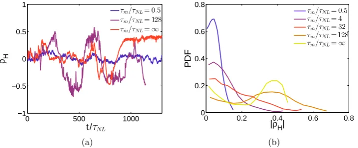
Figure 2: (Color online) (a) Time series of relative helicityρHand (b) Probability Density
Function (PDF) of the absolute value ofρH for the flows with different forcing memory
time scale at Rossby numberRof = 0.1 and Reynolds numberRef = 333
with τm/τN L = 0.5 throughout the duration of the simulation for two reasons. The first reason is due to the short memory timescale of the forcing that keeps the hu·fi
correlation small and the second reason is due to the low Rossby number, resulting in a weak turbulent cascade as we show later on.
3.2. The role of helicity
Helicity is common in real flows and it can be created, for example, in planetary atmo-spheres in the presence of rotation and stratification (Moffatt 1978; Tobias 2009; Marino et al. 2013). In homogenenous non-rotating turbulence it is expected that the helicity spectrum cannot develop if it is initially zero (Andr´e & Lesieur 1977) or if an external mechanism does not inject net helicity (Dallaset al.2015). In our runs zero net helicity is injected into the flow. Nevertheless, for a given rotation rate (i.e.Rof = 0.1) we observe
that the relative helicity ρH = H/(|u||ω|) increases as the memory time scale of the
forcing increases (see Fig. 2).
It is apparent from Fig. 2 that the mirror-symmetry breaking depends on the value ofτm. Figure 2a shows ρH to be almost zero at early times for all the flows and as τm
increases the mirror-symmetry breaks at later times only for long enoughτm. We observe
that helicity emerges in the flow as soon asτmbecomes of the order of the eddy turnover
time, i.e.τm/τN L∼ O(1). To analyse further this behaviour ofρHwe plot the Probability
Density Function (PDF) of the time series of the absolute value of relative helicity in Fig. 2b. This plot shows an increase in the mean value of |ρH|and also a broadening of the
tails of the PDFs for longer memory time scales. So, unlike in homogeneous turbulence, helicity can be created in rotating flows by an external force with a sufficiently long memory time scale, even though net helicity is not injected directly into the flow.
To determine whether the breaking of mirror-symmetry, that distinguishes flows with highly random-in-time and time-independent forcings, remains at higher Reynolds num-bers we carried out simulations for the two extreme cases of τm/τN L = 0.5 and∞ at
Ref = 714 andRof = 0.1. Our numerical simulations confirm the persistence of this
be-haviour at higher Reynolds numbers. We therefore analyse these higher Reynolds number runs in order to gain further insight on the effects of helicity on the flow.
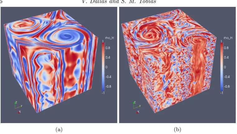
Visualisations of the relative helicity of the flows withRef = 714 are presented in Figs.
[image:6.595.103.468.126.277.2](a) (b)
Figure 3: (Color online) Visualisations of the relative helicityρH for the flows at Rossby
number Rof = 0.1 and Reynolds number Ref = 714 with (a) τm/τN L = 0.5, ρH = −0.018 and (b)τm/τN L=∞,ρH= 0.45
The red and blue colour in Fig. 3 indicate right-hand (positive helicity) and left-hand (negative helicity) circularly polarized helical waves, respectively. An instructive way to explain this further is to decompose the velocity field into circularly polarised helical waves (Constantin & Majda 1988; Waleffe 1992)
u(x, t) =h±(k)ei(
k·x−ω±t), (3.1)
whereik, h+andh− are the linearly independent eigenvectors of the curl operator, i.e.
ik×h± = ±|k|h±. These complex eigenvectors are orthogonal to each other and are
fully helical. So, nowub(k) can be expressed as a linear combination of the eigenvectors
h+ andh− only as follows
b
u(k, t) =u+(k, t)h+(k) +u−(k, t)h−(k) (3.2)
sincek·ub(k) = 0. Then, the helicity can be separated into modes of positive and negative helicity, viz.
H =X
k
b
u(k)·ωb∗(k)
=X
k
k(|u+(k)|2− |u−(k)|2)
=k(E+−E−) =H+−H−, (3.3)
where∗ denotes the complex-conjugate.
[image:7.595.97.478.109.324.2]k⊥
50 100 150 kk
50 100 150
(a)
k⊥
50 100 150 kk
50 100 150
(b)
Figure 4: (Color online) The two-dimensional energy spectrumE2D(k⊥, kk) for the flows
at Rossby numberRof = 0.1 and Reynolds number Ref = 714 with (a)τm/τN L= 0.5,
ρH=−0.018 and (b)τm/τN L=∞,ρH= 0.45
and intermediate scales that is imposed by rotation (see Fig. 3b). Note that the two large scale vortices are still present but this time they have the same sign of helicity on average. Similar effects of helicity have also been observed on an elder study of decaying rotating turbulence (Morinishiet al.2001).
In order to quantify the level of anisotropy of these two runs we consider the 2D energy spectrum which is defined as
E2D(k⊥, kk) =
X
kk6|k·ez|<kk+1
k⊥6|k×ez|<k⊥+1
|ukb |2. (3.4)
The sum is restricted here at energy in cylinders of radius k⊥ and energy in planes
kk. Figures 4a and 4b show the 2D energy spectrum for the flows with τm/τN L = 0.5
and ∞, respectively. The contours of the 2D energy spectrum for an isotropic flow is represented by concentric circles centered at the origin of the axes. Any deviation from the circular pattern indicates the level of anisotropy in the flow.By comparing the two contour plots ofE2D, it becomes clear that in Fig. 4b the intermediate and small scales are closer to isotropy, implying that the flow with the time-independent forcing is overall less anisotropic than the flow with the highly random-in-time forcing.This observation is in agreement with the visualisation of Fig. 3, which prompt us to postulate that the helicity plays a central role on the suppression of anisotropy in the flow.
3.3. Spectral behaviour
In this section we present the spectra of the energyE(k) and the energy flux ΠE(k). The
energy spectrum was spherically averaged using the following expression
E(k) = X
k6|k|<k+1
|ukb |2 (3.5)
and the spectrum of the energy flux was obtained as
ΠE(k) = K X
k=1 X
k6|k|<k+1 b
u∗(k)·(u\×ω)(k). (3.6)
[image:8.595.129.477.100.263.2]100 101 102 10−2
100 102
E(k)∝k−5/3
E(k)∝k−2
k
k
5/2
E(k)
τm/τNL= 0.5 τm/τNL= 4 τm/τNL= 32
τm/τNL= 128
τm/τNL=∞
(a)
100 101 102
−0.5 0 0.5 1
Π E
(k)/
ε E
k
(b)
Figure 5: (Color online) (a) Energy spectraE(k) compensated byk5/2and (b) the energy flux spectra ΠE(k) normalised with the dissipation rateǫEfor flows with different forcing
memory time scale at Rossby numberRof = 0.1 and Reynolds numberRef = 333
that the flow with the time-independent forcing (τm/τN L=∞) was time-averaged only
after∼800τN Lturnover times, when the new steady state was reached (see Fig. 1b).
Note that we did not observe any differences to the scalings of the spectra when averaging over spheres and over cylinders. This has also been shown clearly by Mininni et al.(2009), who performed simulations at low Rossby numbers and of similar resolutions to us. So, the scalings of the spectra that we present are also valid for energy spectra as a function of k⊥. However, significant differences in the scalings are observed in the kk
direction.
The effects of the memory time scale of the forcing is also apparent on the spectral dynamics of our flows. Figure 5a shows the energy spectra of the flows with different memory time scales of the forcing compensated byk5/2. The spectra of these flows obey different power laws which clearly depend on the memory time scale of the forcing. The runs that are forced with the highly random-in-time forcingseem to have ak−5/2
scaling. As τm increases the spectra start to deviate gradually from the k−5/2 scaling
towards ak−2 and finally reach ak−5/3 scaling for the flow with the time-independent forcing. Thek−5/3energy spectrum can be interpreted from the fact that the intermediate and small scales of the flow are closer to isotropy (see Figs. 4b and 3b) and hence we expect the Kolmogorov phenomenology to be valid in this case. All the exponents that we observe here could be related to the various phenomenologies on strong and weak-wave turbulence in the literature, where the interplay between τN L and the time scale
of the inertial waves τw ∝ Ω−1 is central to obtain the different energy spectra. These
spectral exponents have also been observed in other studies of forced rotating flows (Yeung & Zhou 1998; Mininni & Pouquet 2010; Alexakis 2015).Owing to the moderate resolution of these simulations, the statements about the exact spectral exponents are qualitative. In any case, our results show clearly a dependence of the spectra on the nature of the forcing in rotating turbulence. Simulations integrated for extremely long times with higher Reynolds numbers but also lower Rossby numbers, falling in the same dynamical regime of the two-dimensional parameter space, are necessary to verify whether our results imply a lack of universality in these flows.
The corresponding spectra for the energy flux ΠE(k) normalised by the energy
[image:9.595.98.466.102.279.2]a forward cascade while the negative flux indicates a transfer of energy from the small to the large scales of the flow. In the case of negative flux we do not talk about a cascade because we do not have enough scale separation between the forcing scale and the box size. As the memory time scale of the forcing increases, the forward cascade becomes stronger. On the other hand, the flux of energy towards the large scales increases as the forcing becomes more random-in-time with the flow reaching a quasi-2D state. These observations are in line with the visualisations of Fig. 3.
We already saw that, as the forcing becomes less time-dependent helicity increases considerably in our flows, so these changes in the spectra can also be related to the presence of strong net helicity in the flow. This is in agreement with prior studies that have shown the influence of helicity on the energy spectrum by directly injecting helicity into the flow (Mininni & Pouquet 2009, 2010). In contrast, helicity does not seem to have any significant effect on the spectra in non-rotating, homogeneous and isotropic helical turbulence (Dallaset al.2015).
The fact that helicity is not a sign-definite quantity and because we do not inject any net helicity, the sign of helicity in our flows undergoes changes in its inertial range. Therefore, there is either no power-law or difficult to define one in our helicity spectra. For this reason, we do not show any helicity spectra here. In the next section, we examine the Rossby number dependence of the dynamics of the flows.
4. Rossby number dependence
4.1. Global behaviour
In the previous sections we saw that the dynamics depend on the nature of the forcing for a given Rossby number. Here, we investigate the effects of the rotation rate on the flows, focusing on the extreme cases of the forcing being highly random-in-time (τm/τN L =
0.5) and time-independent (τm/τN L =∞) for fixed Ref = 333. Again here we restrict
ourselves to moderate Reynolds numbers because extremely long integration times for the runs with time-independent forcing are inevitable.
For high Rossby number flows the effect of rotation is negligible and the energy is expected to flow to scales smaller than the forcing scale. However, as Rossby number is decreased and the flow tends to become quasi-2D, there is more and more energy transferred to scales larger than the forcing scale due to an inverse cascade (Pouquet et al.2013).
We examine the energy and the relative helicity for runs with different Rossby numbers. The triangles and circles denote runs forced with a time-independent forcing and random-in-time forcing, respectively. As Rossby number is decreased we see that energy increases as expected (see Fig. 6a). However, the rate of increase and the values of energy for high enough rotation rates depend on the nature of the mechanical force. Note that the flow with the time-independent forcing has much more energy at small Rossby numbers.
The relative helicity behaves also very differently for the two types of flows and this is shown in Fig. 6b. The flow with the random-in-time forcing has zero net helicity for all Rof. However, the flow with the time-independent forcing bifurcates to a state of
non-zero helicity for small enough Rossby numbers. The value of |ρH| seems to vary
discontinuously as Rof is decreased with the flow bifurcating to a helical state at the
critical Rocrit
f ≃0.2. Thus, the transition from the non-helical to the helical state is a
jump bifurcation. In summary, net helicity emerges in the flow only for small enough
Rof and long enoughτm.
10−2 10−1 100 100
101 102
E
Rof
(a)
10−2 10−1 100
0 0.2 0.4 0.6
|
ρ H
|
Rof
(b)
Figure 6: (Color online) Rossby number dependence of (a) energy and (b) absolute value of relative helicity for flows with Reynolds number Ref = 333. The and △ denote
runs forced withτm/τN L= 0.5 andτm/τN L=∞, respectively.
(i.e.u·(∇×f)6= 0) by a helical mechanical force or if another pseudoscalar quantity exists related to the pseudovector ∇×f. In our work, we observe that net helicity
emerges in rapidly rotating flows with long enough memory time scale forcings only. So, a pseudovector that relates the rotation vector with the forcing isΩ×(∇×f) and hence
the pseudoscalar quantity that will allow the generation of helicity in a rotating flow is
H ∝u·Ω×(∇×f). (4.1)
A similar expression was derived in a different way by Hide (1975) for a rapidly rotating flow in geostrophic balance assuming that the non-linear term is negligible. Now, from Eq. (4.1) we can deduce that no net helicity will be generated for a short memory time scale forcing since h∇×fit = 0 (with h.it denoting an average over time), assuming
isotropy and ergodicity. On the other hand, for a forcing with long enough memory time scaleh∇×fit=g(x)6= 0 and thereforeH 6= 0 for long enough integration time scales
in agreement with our observations.
Moffatt (1970) suggested that a random superposition of inertial waves will exhibit a lack of mirror-symmetry if and only if there is a mechanical excitation on a preferred direction in the propagation of the waves with respect to the axis of rotation. Otherwise, the random superposition of inertial waves in equal proportions would give zero net helicity. Based on Eq. (4.1), we conjecture that such a mechanism is pertinent to our flows where the angle ϕ between Ωez and ∇×f is fixed at time t = 0 for a
time-independent forcing and hence such a forcing can add a preferred direction of propagation to the inertial waves inducing the mirror-symmetry breaking in our flows. From the other side, a highly random-in-time forcing can excite inertial waves on all directions in equal proportions since ϕis random in time and this is why the net helicity remains zero for any value ofRof in this case.
4.2. Spectral behaviour
Here we analyse the energy spectra of the flows at different Rossby numbers. In Fig. 7a we present the energy spectra E(k) compensated by k5/2 of the flows with the highly random-in-time forcing. ForRof = 0.5 the energy spectrum is close to the Kolmogorov
[image:11.595.98.465.106.278.2]100 101 102 10−2
10−1 100 101 102
E(k)∝k−5/3
k
k
5/2
E(k)
Rof=0.5
Rof=0.2
Rof=0.1
Rof=0.05
Rof=0.01
(a)
100 101 102
10−1 100 101
102 E(k)∝k−
5/3
k
k
5/2
E(k)
Rof=0.5
Rof=0.2
Rof=0.1
Rof=0.05
Rof=0.01
(b)
Figure 7: (Color online) Energy spectraE(k) compensated byk5/2for the flows with (a)
τm/τN L= 0.5 and (b)τm/τN L=∞at different Rossby numbers and Reynolds number
Ref = 333
the dominant timescale and then the spectrum is changed to the weak-wave turbulence prediction ofE(k)∝k−5/2 .
Similar behaviour is observed for the spectra of the flows with the time-independent forcing (see Fig. 7b) but with two different characteristics. The first is the significant condensation of energy at large scales for small enough Rossby numbers in comparison to the flows with the random-in-time forcing. The second is the transition from the Kolmogorov-like regime withτE ≪τwto the weak-wave turbulence regime withτw≪τE,
which occurs at lower Rossby numbers, showing the dependence of this transition to the nature of the mechanical force.
Here, we should point out that weak-wave turbulence theory arguments, which assume uniform and isotropic forcing, predict ak−5/2spectrum but they do not predict conden-sation of energy at large scales due to an inverse cascade in unbounded domains. This is in agreement with Fig. 7a where there is some energy condensation at large scales but not significant in comparison to Fig. 7b. However, the energy condensation at large scales in Fig. 7b suggests that weak-wave turbulence theory is not necessarily valid for the small Rossby number flows with time-independent forcing even thoughE(k)∝k−5/2.
5. Discussion & conclusions
The dependence of the dynamics of rotating turbulence on the nature of the large scale mechanical force is studied by means of numerical simulations to shed light on the disparate results in the literature. For moderate Reynolds and low Rossby number flows we systematically vary the memory time scaleτmof the mechanical force. Asτmincreases
the forcing mechanism becomes less time-dependent and essentially less isotropic. We are able to demonstrate that different steady state solutions will be reached if one is able to integrate for long enough time scales, showing the dependence of the flows on the forcing mechanism. When τm ∝ τN L we observe that mirror-symmetry spontaneously breaks
in the flow even though our mechanical force is non-helical. Moreover, as the forcing mechanism becomes less time-dependent (longτm) the net helicity increases. This is also
[image:12.595.101.466.120.278.2]makes the flow less anisotropic in contract to a flow with highly random-in-time forcing where the net helicity appears to be negligible.
In addition, for moderateRef and lowRof flows both the power laws for the energy
spectrum and the forward and inverse fluxes of energy depend strongly on the forcing mechanism.Depending on the value ofτmwe obtain different scaling of the energy spec-trum with E(k) ∝ k−5/3, k−2 and k−5/2 showing a clear dependence of the spectral
dynamics on the nature of the external driving force. Alexakis (2015) showed that no matter how large the Reynolds number can be there is a small enough Rossby num-ber such that the flow exhibits a particular behaviour (e.g. weakly rotating turbulence, quasi-2D condensates) provided that an appropriateα >0 is considered in the scaling
Rof ∝ Re−fα (where α is expected to depend on the external driving force). So, lack
of universality seems plausible in forced rotating turbulent flows. To corroborate this argument a large extent of the control parameters space should be covered with higher Reynolds number and lower Rossby number simulations integrated for extremely long times.However, this is beyond the reach of current computational capabilities.
The Rossby number dependence on the dynamics of flows with a highly random-in-time and a random-in-time-independent mechanical force is also investigated at moderate Reynolds numbers. For weakly rotating turbulence (highRof) the total energies of the two systems
are comparable. Even so for small enough Rof, even though large scale vortices are
present in both systems, energy condensates at large scales only for the flow with the time-independent forcing as the energy spectra demonstrate.
Moreover, for large Rof the net felicities of the two systems are zero but as Rof
becomes smaller there is a critical Rocrit
f which the flow with the time-independent
forcing bifurcates discontinuously from a non-helical state to a helical state. On the other hand, the helicity of the flow with the random-in-time forcing remains zero for all values ofRof. Based on this observation we argue that the angle between Ωezand∇×f
is important on the excitation of the inertial waves and consequently on the generation of net helicity in rotating flows. Thus, a time-independent forcing adds a preferred direction of propagation to the inertial waves inducing the mirror-symmetry breaking in our flows, since this angle is fixed in time. From the other side, a highly random-in-time forcing with excites inertial waves on all directions in equal proportions and this is why the net helicity remains zero for any value ofRof. Such a mechanism has also been proposed for
planetary dynamos (Moffatt 1970).
In the end, the lack of consistency of the results in the literature is attributed here on the forcing-depend dynamics of forced rotating turbulent flows. Experiments should be able to show if this is true at higher Reynolds and lower Rossby numbers. The spon-taneous emergence of helicity in such flows is an important aspect with implications on cyclones persistence and intensity in supercell thunderstorms, a phenomenon which defies weather forecasting (Markowskiet al.1998) but also in planetary dynamos.
Acknowledgements
REFERENCES
Alexakis, A.2015 Rotating taylor-green flow.Journal of Fluid Mechanics 769, 46–78.
Andr´e, J. C. & Lesieur, M.1977 Influence of helicity on the evolution of isotropic turbulence at high reynolds number.Journal of Fluid Mechanics81, 187–207.
Bartello, Peter, M´etais, Olivier & Lesieur, Marcel1994 Coherent structures in rotating three-dimensional turbulence.Journal of Fluid Mechanics 273, 1–29.
Bewley, Gregory P., Lathrop, Daniel P., Maas, Leo R. M. & Sreenivasan, K. R.2007 Inertial waves in rotating grid turbulence.Physics of Fluids19, 071701,.
Boffetta, Guido & Ecke, Robert E.2012 Two-dimensional turbulence.Annual Review of Fluid Mechanics44(1), 427–451.
van Bokhoven, L. J. A., Clercx, H. J. H., van Heijst, G. J. F. & Trieling, R. R.2009 Experiments on rapidly rotating turbulent flows.Physics of Fluids 21, 096601.
Bracco, Annalisa & McWilliams, James C.2010 Reynolds-number dependency in homo-geneous, stationary two-dimensional turbulence.Journal of Fluid Mechanics646, 517–526.
Cambon, Claude, Mansour, N. N. & Godeferd, F. S. 1997 Energy transfer in rotating turbulence.Journal of Fluid Mechanics337, 303–332.
Constantin, Peter & Majda, Andrew1988 The beltrami spectrum for incompressible fluid flows.Communications in Mathematical Physics115, 435–456.
Dallas, V. & Alexakis, A.2015 Self-organisation and non-linear dynamics in driven magne-tohydrodynamic turbulent flows.Physics of Fluids 27, 045105.
Dallas, V., Fauve, S. & Alexakis, A.2015 Statistical equilibria of large scales in dissipative hydrodynamic turbulence.Phys. Rev. Lett.115, 204501.
Davidson, P. A., Staplehurst, P. J. & Dalziel, S. B.2006 On the evolution of eddies in a rapidly rotating system.Journal of Fluid Mechanics557, 135–144.
Deusebio, E., Boffetta, G., Lindborg, E. & Musacchio, S.2014 Dimensional transition in rotating turbulence.Phys. Rev. E 90, 023005.
Dombre, T., Frisch, U., Greene, J. M., Hnon, M., Mehr, A. & Soward, A. M. 1986 Chaotic streamlines in the abc flows.Journal of Fluid Mechanics 167, 353–391.
Galtier, S´ebastien2003 Weak inertial-wave turbulence theory.Phys. Rev. E 68, 015301.
G´omez, Daniel O., Mininni, Pablo D. & Dmitruk, Pablo 2005 Parallel simulations in turbulent MHD.Physica ScriptaT116, 123–127.
Greenspan, H. P.1968The Theory of Rotating Fluids. Cambridge University Press.
Hide, R.1975 A note on helicity.Geophysical Fluid Dynamics 7(1), 157–161.
Hopfinger, E J & Heijst, G J F V1993 Vortices in rotating fluids.Annual Review of Fluid Mechanics 25, 241–289.
Hossain, Murshed1994 Reduction in the dimensionality of turbulence due to a strong rotation.
Physics of Fluids 6, 1077–1080.
Kolmogorov, A. N.1941 The local structure of turbulence in incompressible viscous fluid for very large Reynolds number.Doklady Akademii Nauk SSSR30, 301–305.
Lighthill, James1965Waves in fluids. Cambridge University Press.
Maltrud, M. E. & Vallis, G. K. 1991 Energy spectra and coherent structures in forced two-dimensional and beta-plane turbulence.Journal of Fluid Mechanics228, 321–342.
Marino, Raffaele, Mininni, Pablo D., Rosenberg, Duane & Pouquet, Annick 2013 Emergence of helicity in rotating stratified turbulence.Phys. Rev. E 87, 033016.
Markowski, Paul M, Straka, Jerry M, Rasmussen, Erik N & Blanchard, David O1998 Variability of storm-relative helicity during VORTEX.Monthly weather review 126(11), 2959–2971.
Mininni, P. D., Alexakis, A. & Pouquet, A. 2009 Scale interactions and scaling laws in rotating flows at moderate rossby numbers and large reynolds numbers.Physics of Fluids
21, 015108.
Mininni, P. D. & Pouquet, A.2009 Helicity cascades in rotating turbulence. Phys. Rev. E
79, 026304.
Mininni, P. D. & Pouquet, A. 2010 Rotating helical turbulence. i. global evolution and spectral behavior.Physics of Fluids 22, 035105.
Moffatt, H. K. 1970 Dynamo action associated with random inertial waves in a rotating conducting fluid.Journal of Fluid Mechanics44, 705–719.
Moffatt, Henry K.1978Magnetic Field Generation in Electrically Conducting Fluids. Cam-bridge University Press.
Moisy, F., Morize, C., Rabaud, M. & Sommeria, J. 2011 Decay laws, anisotropy and cyclone-anticyclone asymmetry in decaying rotating turbulence.Journal of Fluid Mechan-ics 666, 5–35.
Morinishi, Youhei, Nakabayashi, Koichi & Ren, Shuiqiang 2001 Effects of helicity and system rotation on decaying homogeneous turbulence.JSME International Journal Series B Fluids and Thermal Engineering44, 410–418.
Pouquet, A. & Mininni, P. D.2010 The interplay between helicity and rotation in turbulence: implications for scaling laws and small-scale dynamics. Philosophical Transactions of the Royal Society of London A: Mathematical, Physical and Engineering Sciences368(1916), 1635–1662.
Pouquet, A, Sen, A, Rosenberg, D, Mininni, P D & Baerenzung, J2013 Inverse cascades in turbulence and the case of rotating flows.Physica ScriptaT155, 014032.
Proudman, J.1916 On the motion of solids in a liquid possessing vorticity.Proceedings of the Royal Society of London A: Mathematical, Physical and Engineering Sciences 92(642), 408–424.
Ruppert-Felsot, Jori E., Praud, Olivier, Sharon, Eran & Swinney, Harry L. 2005 Extraction of coherent structures in a rotating turbulent flow experiment. Phys. Rev. E
72, 016311.
Sen, Amrik, Mininni, Pablo D., Rosenberg, Duane & Pouquet, Annick2012 Anisotropy and nonuniversality in scaling laws of the large-scale energy spectrum in rotating turbu-lence.Phys. Rev. E 86, 036319.
Smith, Leslie M., Chasnov, Jeffrey R. & Waleffe, Fabian1996 Crossover from two- to three-dimensional turbulence.Phys. Rev. Lett.77, 2467–2470.
Taylor, G. I.1917 Motion of solids in fluids when the flow is not irrotational.Proceedings of the Royal Society of London A: Mathematical, Physical and Engineering Sciences93(648), 99–113.
Teitelbaum, Tomas & Mininni, Pablo D. 2011 The decay of turbulence in rotating flows.
Physics of Fluids 23(6), 065105.
Tobias, S. M.2009 The solar dynamo: The role of penetration, rotation and shear on convective dynamos.Space Science Reviews144, 77–86.
Tritton, D. J.1988 Physical fluid dynamics.Oxford, Clarendon Press .
Waleffe, Fabian1992 The nature of triad interactions in homogeneous turbulence.Physics of Fluids A4(2), 350–363.
Yeung, P. K. & Zhou, Ye1998 Numerical study of rotating turbulence with external forcing.
Physics of Fluids 10, 2895–2909.
Yoshimatsu, K., Midorikawa, M. & Kaneda, Y.2011 Columnar eddy formation in freely decaying homogeneous rotating turbulence.Journal of Fluid Mechanics 677, 154–178.