This is a repository copy of
A Comparison of Methods for Representing Random Taste
Heterogeneity in Discrete Choice Models
.
White Rose Research Online URL for this paper:
http://eprints.whiterose.ac.uk/43631/
Article:
Fosgerau, M and Hess, S (2009) A Comparison of Methods for Representing Random
Taste Heterogeneity in Discrete Choice Models. European Transport - Trasporti Europei,
42. 1 - 25 . ISSN 1825-3997
Reuse
Unless indicated otherwise, fulltext items are protected by copyright with all rights reserved. The copyright exception in section 29 of the Copyright, Designs and Patents Act 1988 allows the making of a single copy solely for the purpose of non-commercial research or private study within the limits of fair dealing. The publisher or other rights-holder may allow further reproduction and re-use of this version - refer to the White Rose Research Online record for this item. Where records identify the publisher as the copyright holder, users can verify any specific terms of use on the publisher’s website.
Takedown
If you consider content in White Rose Research Online to be in breach of UK law, please notify us by
A comparison of methods for representing random
taste heterogeneity in discrete choice models
Mogens Fosgerau ∗ Stephane Hess † January 22, 2008
Abstract
This paper reports the findings of a systematic study using Monte Carlo experiments and a real dataset aimed at comparing the performance of vari-ous ways of specifying random taste heterogeneity in a discrete choice model. Specifically, the analysis compares the performance of two recent advanced approaches against a background of four commonly used continuous distribu-tion funcdistribu-tions. The first of these two approaches improves on the flexibility of a base distribution by adding in a series approximation using Legendre polynomials. The second approach uses a discrete mixture of multiple con-tinuous distributions. Both approaches allows the researcher to increase the number of parameters as desired. The paper provides a range of evidence on the ability of the various approaches to recover various distributions from data. The two advanced approaches are comparable in terms of the likeli-hoods achieved, but each has its own advantages and disadvantages.
Keywords: random taste heterogeneity, mixed logit, method of sieves, mix-tures of distributions
∗Technical University of Denmark, Copenhagen, [email protected]
1
Introduction
The widespread use of models such as the Mixed Multinomial Logit (MMNL) model (cf.Revelt and Train,1998;Train,1998;McFadden and Train,2000; Hen-sher and Greene, 2003; Train, 2003) has made the issue of choosing a mixing distribution very important. In these models we must specify a mixing distri-bution, i.e. a distribution of random parameters, that may be interpreted as representing random taste heterogeneity. The trouble is that we never observe these random parameters and that we mostly have little a priori information about the shape of their distribution except possibly a sign constraint. On the other hand, the choice of a specific distribution may seriously bias results if that distribution is not suitable for the data (cf. Hess et al., 2005; Fosgerau, 2006). This kind of misspecification is particularly damaging when the distribution is it-self of interest as is the case in estimation of the value of travel time, the response to tolls, adoption of a new mode, etc.1
The point of this paper is to provide a comparison of two advanced approaches for the representation of random taste heterogeneity in discrete choice models. A prominent feature of the paper is the graphical evidence we provide on the ability of the various approaches to approximate various challenging distributions. The range of possible shapes of the mixing distribution is determined by a number of deep parameters to be estimated. The two advanced approaches in this paper are ways of specifying the mixing distribution with a variable number of deep parameters such that an arbitrary level of flexibility may be achieved. In the present paper, we limit our attention to univariate mixing distributions2
; the use of multivariate distributions is a topic for further research.
Various authors have estimated a range of parametric distributions, aiming to gauge the advantages of distributions with a high degree of flexibility (see for example Hensher and Greene, 2003; Train and Sonnier, 2005; Hess et al., 2006). However, although different distributions have different properties, flexi-bility is generally determined by the number of parameters for the distributions. A two-parameter distribution corresponds to just a two-dimensional subset of some space of distributions. So, while it may be possible to find a low-parameter parametric distribution that fits well in a specific situation, it will not be more flexible than other parametric distributions with the same number of parameters. This acts as our main motivation for exploring alternative ways of representing random taste heterogeneity.
1Misspecification has even lead some researchers to think that they have evidence of positive
marginal utility of travel time, when in fact they have just specified a mixing distribution that has values on both sides of zero.
The method of sieves is a natural choice for generating flexible distribu-tions. Consider some model containing an unknown function to be estimated, where, in the present case, the unknown function is the unknown density of a taste coefficient α. The unknown function can be thought of as a point in an infinite-dimensional parameter space. Rather than trying to estimate a point in an indimensional space, one estimates over an approximating finite-dimensional parameter space. As the dimension of the approximating space grows, the resulting estimate approaches the true unknown function under quite general circumstances (Chen,2006). Additionally, the dimension of the imating space can increase with the size of the dataset such that better approx-imations to the true function are obtained for larger datasets. In econometrics, the resulting estimators are known as semi-nonparametric (Gallant and Nychka, 1987).
There are various ways of approximating an infinite-dimensional space of dis-tributions by finite-dimensional spaces. In this paper, we shall confine attention to just two convenient possibilities and we shall fix the number of parameters to be estimated, corresponding to the dimension of the approximating space, at low values. What we obtain is thus just some very flexible distributions with more parameters than usual. The distributions can be extended with more parameters as desired in a very straightforward way, as discussed in Section2.
The first approach we consider is that described by Fosgerau and Bierlaire (2007). The main feature of this approach is that it can use any continuous distribution as its base. This is then extended by means of a series expansion, in our case using Legendre polynomials, such that any continuous distribution can be approximated at the limit, providing it has support within the support of the base distribution. The number of parameters can be increased one by one by increasing the number of terms used in the series expansion. Fosgerau and Bierlaire(2007) present the technique as a test of the appropriateness of the base distribution, used by testing the model with additional terms against the base model. Here, we simply use the resulting model as a flexible means of retrieving random taste heterogeneity.
mix-tures of Normal distribution is given byGeweke and Keane (2001).
Both approaches have the flexibility of allowing for multiple modes in a dis-tribution. This can be a significant advantage compared to the typically used distributions (e.g. Normal, Lognormal, ...) that are restricted to a single mode, given the possibility that the sample may be composed of distinct groups with different behaviour.
In this paper, we present evidence from two separate studies. In the first part of the paper, we conduct a systematic study using Monte Carlo experiments. Here, we show that the two flexible approaches are both able to approximate well a range of true distributions, even though the number of deep parameters is kept reasonably low. The two approaches do about equally well in outperforming four commonly used distributions over a range of situations. Hence, we recommend the use of a flexible approach in applied modelling work, at least as a guide to the selection of a simpler distribution. The choice between the two flexible approaches may be guided by considerations on bias and variance, which seem to favour the Fosgerau & Bierlaire approach, or by the ability of the MOD estimator to approximate point masses.
In the second part of the paper, we provide evidence on the methods using data from the Swiss value of time study. Here we simultaneously estimate flexible distribution for four coefficients, which we believe is a first. We find the appli-cation of the flexible approaches to be illuminating in that it reveals features of the data that could not be revealed using the simpler approaches. The MOD ap-proach did run into a limitation in that it turned out to be not computationally possible to estimate beyond a mixture of two normals for each coefficient. On the other hand, a larger number of parameters could be estimated with the Fosgerau & Bierlaire approach, with no limit in sight.
We do not provide theoretical results concerning consistency and asymptotic properties of the estimators of the distribution of α that we employ. Fosgerau and Nielsen(2006) prove consistency of an estimator of the distribution of α in a case when the distribution of the error terms3
is unknown. It seems feasible to extend this result to the case of a MMNL model with an unknown mixing distribution.
The paper is organised as follows. The following section presents the math-ematical details of the two advanced approaches used in this paper. This is followed in Section3by a discussion of the results from the Monte Carlo studies, and a discussion of the results from the application on real data in Section 4. Finally, Section5presents the conclusions of the analysis.
2
Methodology
In this section, we discuss the two main methods compared in this analysis, with the Fosgerau-Bierlaire approach described in Section2.1, and the MOD approach described in Section2.2. This is followed in Section2.3by a brief description of various continuous distributions used in our experiments.
2.1 Fosgerau & Bierlaire approach
Let Φ be the standard Normal cumulative distribution function with density φ
and letG be an absolute continuous distribution with density g. We take Φ as the base distribution with which we seek to estimate the true distributionG.4
Since both Φ andGare increasing, it is possible to defineQ(x) =G(Φ−1 (x)) such that Q(Φ(β)) = G(β). Furthermore, Q is monotonically increasing and ranges from 0 to 1 on the unit interval. Thus, Q is a cumulative distribution function for a random variable on the unit interval. Denote by q the density of this variable, which exists since Gis absolute continuous. Then we can express the true density asg=q(Φ)φ.
Consider now a discrete choice model P(y|v, α) conditional on the random parameterα which has the true distributionG. Then the unconditional model is
P(y|v) =
Z
α
P(y|v, α)g(α)dα
=
Z
x
P(y|v,Φ−1
(x))q(x)dx (1)
Thus the problem of finding the unknown densityg is reduced to that of finding
q, an unknown density on the unit interval. The terms Φ−1
(x) are just standard Normal draws used in numerical simulation of the likelihood (cf.Train,2003).
Now, letLk be the kthLegendre polynomial on the unit interval (cf. Bierens,
2007; Fosgerau and Bierlaire,2007). These functions constitute an orthonormal base for functions on the unit interval5
such that R LkLk′ is equal to 1 when
k=k′ and zero otherwise. We can then write
q(x) = (1 +
P
kγkLk)2
1 +Pkγ2
k
. (2)
Squaring the numerator ensures positivity, while the normalisation in the denom-inator ensures thatq(x) integrates to 1. Thus this expression is in fact a density.
4It is generally appropriate to choose a base distribution that is a priori thought to be a likely
candidate for the true distribution. We choose the Normal distribution to have consistency with the MOD approach.
Bierens(2007) proves that any density on the unit interval can be written in this way.
The choice of Legendre polynomials is not a necessity. There are many other bases for functions on the unit interval that could have been used. Legendre polynomials are convenient because they have a recursive definition that is easily implemented on a computer.6
To define the estimator that we use in this paper, we simply select a cut-offK
fork, such that we only use the firstKterms of (2). Thus we have a representation of a flexibleqK with K parameters and a corresponding cumulative distribution
functionQK. This is inserted into equation (1) to enable estimation by maximum
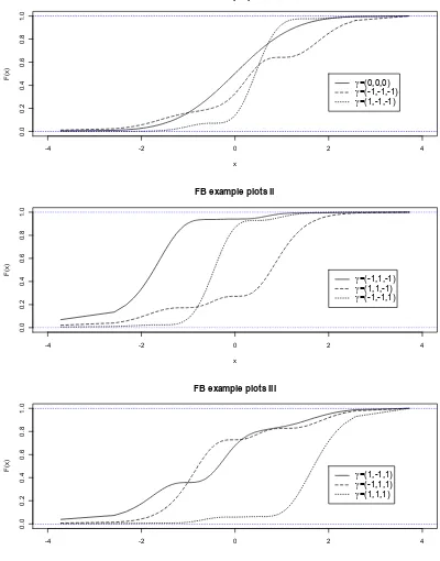
likelihood. For more details on this approach, seeFosgerau and Bierlaire(2007). Figure1shows cumulative distribution functions (CDF) for various parameter combinations of aQ3(Φ) distribution, where the base distribution Φ is a standard Normal distribution and the threeγk parameters are set to all combinations of
-1, 0 and 1. As the figure shows, this general form is able to take a variety of shapes.
2.2 Mixtures of distributions approach
In our MOD approach, we combine a standard continuous mixture approach with a discrete mixture approach, as described for example byHess et al.(2007) and, in another context,Coppejans(2001). Specifically, the mixing distribution is itself a discrete mixture of several independently distributed Normal distributions. We define a set of mean parameters, µk and a corresponding set of standard
deviations, σk, with k = 1, . . . , K. For each pair (µk, σk), we then define a
probabilityπk, where 0≤πk ≤1, ∀k, and wherePKk=1πk= 1. A draw from the
mixture distribution is then produced on the basis of two uniform drawsu1 and
u2 contained between 0 and 1, where we get:
α= Φ−µ11,σ1(u1), ifu2 < π1
α= Φ−µk1,σk(u1), if
k−1
X
l=1
πl≤u2<
k X
l=1
πlwith 1< k≤K−1
α= Φ−1
µK,σK(u1), if
KX−1
l=1
πl≤u2, (3)
6The recursion formula for the Legendre polynomials on the unit interval states thatL
k(x) = √
4k2−1
k (2x−1)Lk−1(x)−(
k−1)√2k+1
k√2k−3 Lk−2(x). The first four polynomials areL0(x) = 1,L1(x) = √
3(2x
−1),L2(x) =√5(6x2−6x+ 1), andL3(x) = √
7(20x3
where Φ−1
µk,σk is the inverse cumulative distribution of a Normal with mean µk
and standard deviationσk.
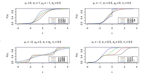
WithkNormal terms, the resulting distribution allows forkseparate modes, where the different modes can differ in mass. However, the flexibility of this approach is not limited to allowing for multiple modes, the method also allows for saddle points in a distribution.
Furthermore, it is possible to have point-mass at a specific value, in which case the associated standard deviation parameter becomes 0. This property of the MOD approach is both a blessing and a curse. Coppejans(2001) enforces a lower bound on the variance of the normally distributed components in order to ensure that the estimated distribution is smooth and to prove asymptotic convergence to the true distribution as the number of Normal distributions increases with sample size. Thus imposing a lower bound on the variances is desirable when the true distribution is thought to be smooth and it avoids the estimated distribution becoming degenerate.
It is difficult to make a case for mass-points in a distribution of preference-parameters. However, there is one exception, namely a heightened mass at zero. This is useful in the representation of taste heterogeneity for attributes that some individuals are indifferent to, a concept discussed for example in the context of the valuation of travel time savings (VTTS) byCirillo and Axhausen (2006). It can also be useful in the context of attribute processing strategies in SP data, with some respondents ignoring certain attributes, such that they obtain a zero coefficient (cf. Hensher, 2006). In the results below we do not impose a lower bound on the variances.
Normal fixed at −2. As the mean of the second Normal is gradually decreased from its initial value of 2, we move from a distribution with two separate peaks to a distribution approximating a Normal.
2.3 Other distributions
Along with the approaches from Section 2.1 and Section 2.2, we also estimated models making use of a set of standard continuous distributions, as commonly used in Mixed Logit analyses. Here, we limit the set of distributions to the Normal, the Uniform, the symmetrical Triangular and the Johnson SB.
3
Experiments on simulated data
This section presents the results from our systematic Monte Carlo analysis. We first present the empirical framework used in this analysis (Section 3.1). We then briefly discuss the issue of the number of parameters (Section 3.2) before discussing the actual results (Section3.3).
3.1 Generation of data
The setup for this analysis makes use of binary choice panel data. The conditional indirect utility function for the first alternative is set to zero, while, in choice situationtfor respondent n, the utility of the second alternative is given by:
Un,t=αn+vn,t+
1
µεn,t, (4)
where ε follows a logistic distribution, vn,t is an observed quantity, and αn is
an individual-specific i.i.d. latent random variable. This is the simplest possi-ble setup that allows us to identify the distribution of an unobserved random parameter. This simplicity is a virtue, since we can then focus on the issue at hand, namely the ability of different estimators to recover a true distribution. The use of panel data is crucial, since otherwise it becomes hard to distinguish the distribution ofα from the distribution ofε.
We simulate datasets of a size that is realistic in applied situations, containing 1,000 “individuals” making 8 “choices” each. We generate data for seven different choices oftruedistribution forαn, with details given below. The observed variable
v is drawn from a standard Normal distribution, while the scale parameter µ is fixed at a value of 2.
Therefore we generate 50 datasets for each distribution.7
Estimating the mod-els many times for each true distribution of α allows us to take into account the fact that the estimates are random variables obtained as functions of random data. Altogether, we generate 50 datasets for each of the seventruedistributions, leading to a total of 350 datasets.
The seventrue distributions were chosen with the aim of representing a wide array of possibilities that challenge our ability to estimate them. An important point here is to select the distributions such that they lie well within the support of vn,t which is standard Normal. Thus we have selected the distributions to lie
mostly within the interval [-2,2].8
Specifically, we use the following seven data generating processes:
DM(2) data: discrete mixture with two support points,α=−1 with probabil-ityπ1 = 0.5, andα= 1 with probability π2 = 0.5
DM(3) data: discrete mixture with three support points, α =−1, α = 0 and
α= 1, with equal mass ofπ1=π2 =π3 = 13
LN data: Lognormal shifted to the left, generated by α=exp(u)/2−1, where
u∼N(0,1)
N data: Standard Normal,α∼N(0,1)
NM data: Normal with point mass at zero. With probability π1 = 0.8, α ∼
N(−1,1), and with probabilityπ2= 0.2, α= 0.
2N data: Mixture of two Normals, with π1 = 0.5, α ∼ N(−1,0.5), and with
π2 = 0.5,α∼N(1,0.5)
U data: Uniform distribution,α∼U[−1,1]
3.2 The number of parameters
The Normal, Uniform and symmetrical Triangular distributions all have just two parameters to be estimated, while the Johnson SB distribution is more flexible with four parameters to be estimated. In addition there is the parameter µ
for the scale of the model. The MOD approach has three parameters for each
7With real data it is possible to use bootstrap methods to generate confidence intervals
around the estimated distribution. These confidence intervals can then be used to learn how much is determined from the data about the estimated distribution.
8This is an issue in real applications, where data may not be sufficiently rich to identify
Normal distribution used (location, variance and mass), less one since the masses sum to one. With a mixture of two Normals there are thus six parameters to be estimated. Therefore we also elect to use a total of six parameters for the Fosgerau-Bierlaire approach. Generally, we expect the ability of a distribution to approximate an arbitrary true distribution to increase with the number of parameters. Thus we expect the worst performance from the Normal, Uniform and symmetrical Triangular distributions, while the best performance is expected from the Fosgerau-Bierlaire approach and the MOD approach.
3.3 Results
In this section, we discuss the results of the Monte Carlo analysis carried out to compare the different methods for representing random taste heterogeneity. All estimation is carried out in Ox (Doornik,2001) using customised code.9
Al-together we have estimated six models10
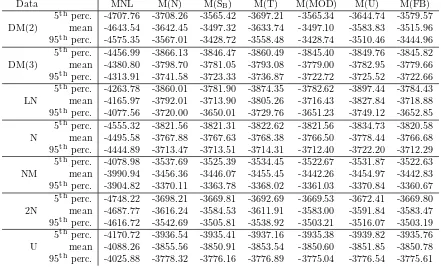
on each of seven datasets, with fifty replications of each dataset. Given the high number of models estimated, only summary results across runs can be presented here. The two advanced models are identified as M(MOD) (mixture of Normals) and M(FB) (Fosgerau-Bierlaire approach), while the four more basic models are identified as M(N) (Normal), M(U)(Uniform), M(T) (symmetrical Triangular) and M(SB) (Johnson SB). In addition, a standard Multinomial Logit (MNL) model was estimated on the data. Two different criteria are used in the presentation of the results. These are the ability to recover the shape of the true distribution and the estimated log-likelihoods. A combination of tables and graphs are used in the presentation of the results.
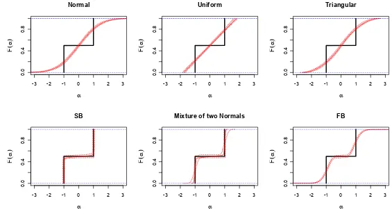
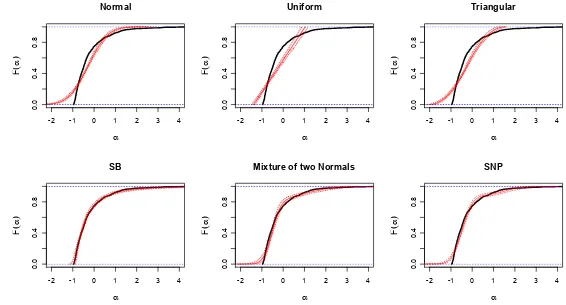
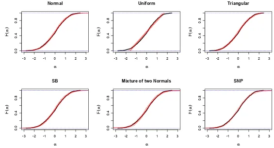
• The performance of the various methods in terms of the recovery of the shape of thetrue distribution is illustrated with the help of CDF plots for thetrue and estimated distributions, where, for the latter, the mean CDF across runs is presented alongside a pointwise 90% confidence band for the CDF. The various plots are shown in Figure3for the DM(2)data, Figure 4for theDM(3)data, Figure5 for theLNdata, Figure6 for theNdata, Figure7 for theNMdata, Figure 8for the2N data, and Figure9 for the
U data.
• These CDF plots are the main result of the analysis as they directly inform on the ability to estimate the unknown true distributions. Vertical distances in the CDF plots correspond to theL∞norm of the difference between true
9Available from the authors on request.
and estimated CDFs; indeed, in the space of CDFs, convergence of estimates to the true distribution, as the number of terms increases, takes place in
L∞ norm. We have chosen to present CDFs rather than densities, since many of the true distributions that we use have point masses and hence no ordinary densities. Moreover, convergence inL∞norm is easier to interpret visually than convergence inL1 norm, which corresponds to densities.
• Table 1 shows the final log-likelihood (LL) obtained in estimation of the various models. Here, we give the mean LL obtained across the fifty runs in each model and dataset combination, along with the 5th
and 95th
percentiles of the distribution of the LL measure across runs, giving an indication of the stability of the methods.
We will now proceed with a discussion of the results obtained in the various datasets.
DM(2) data: For the data generated by a discrete mixture with two support points, we expect the M(MOD) and the M(SB) to perform best due to their ability to become degenerate. The M(MOD) can accommodate the DM(2) distribution with two Normals with zero variance, while the M(SB) can have infinite variance for the Normal distribution.
Figure 3 shows that M(MOD) and M(SB) are able to reproduce the true distribution quite closely. The M(SB) finds the two mass points and puts almost all the mass there through a very large variance of the underlying Normal distribution. The same goes for the M(MOD), which assigns very low variances to the two Normal distributions at the two mass points. The M(FB) is able to indicate roughly the shape of the true distribution but is seemingly not able to generate very sharp kinks in the estimated CDF. Note that the estimated confidence bands are somewhat tighter for the M(FB) than for the M(MOD). The approximations given by M(U), M(T) and M(N) are not able to reveal much about the true distribution except its location and range.
not yield a significant improvement of the mean log-likelihood. But it does allow the M(MOD) to reproduce the true distribution under investigation, in principle perfectly.
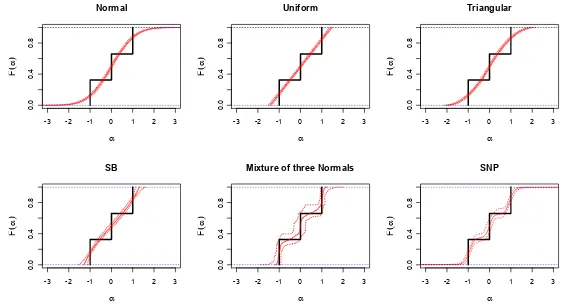
Figure4now shows, as expected, that none of the four simplest distributions are able to provide any information about the true distribution other than its location and rough range. Both the M(MOD) and the M(FB) with the increased number of parameters are able to indicate the shape of the true distribution. The M(MOD) is able to concentrate more of the mass near the three mass points of thetrue distribution but again at the cost of larger confidence bands. In other words, the M(MOD) is able to estimate the true distribution with smaller bias but larger variance.
The log-likelihoods fits obtained by M(MOD) and M(FB) are best, but not much better than M(SB) and M(U).
LN data: For the data generated by a Lognormal distribution, we find in Figure 5 that the two advanced distributions along with the M(SB) are able to recover the lognormal shape quite well. This is quite remarkable, since it implies that a true continuous distribution can be recovered even though it is quite different from the Normal distribution which is used as a base. This should be important in applied work where a priori information about the shape of the true distribution is not available. The M(SB) is even able to find the lower bound on the true distribution. These models produce much better log-likelihoods than the simpler models based on normal, triangular and uniform distributions.
N data: For the data generated with a standard Normal distribution we expect the M(N), M(MOD) and M(FB) to do well, since they nest the true model. Also the M(SB) should do well by letting the range of the distribution be large. This is confirmed by the results in Figure 6. In fact, even the Triangular distribution is able to reproduce the shape of the Normal dis-tribution quite closely. Like before, it seems that the estimated CDF from the M(MOD) has somewhat higher variance than M(FB).
The log-likelihoods are close with only the M(U) doing noticeably worse than the rest. The M(MOD) and M(FB) nest the true distribution and given the small differences in the estimated log-likelihoods, it would be al-most always possible to accept the null hypothesis that the true distribution is in fact Normal, which is reassuring.
is set to zero such that the distribution becomes degenerate.
While all the estimated models are able to indicate the location and range of the true distribution, it is only the M(MOD) that is able to provide a hint about the point mass (Figure 7). The cost is, however, that the M(MOD) again seems to have a higher variance.
In terms of log-likelihoods, the M(MOD) and the M(FB) achieve similar fits, while the M(SB) is somewhat poorer and the remaining are further behind.
2N data: For the data generated by a mixture of two Normals, the MOD model M(MOD) obtains the best model fit. This is as expected since the model is the same as the data generating process. The M(FB) and the M(SB) are however very close. As Figure8 shows, the M(MOD) and also the M(FB) are both able to reproduce the main features of the true 2N distribution. Again, the M(MOD) seems to have higher variance.
U data: For the final dataset, generated with a Uniform distribution, the per-formance of the various models is very similar. From Figure 9, we note that the M(MOD) again has somewhat higher variance than the M(FB) distribution. In terms of log-likelihood, all models are quite similar.
4
Experiment on real data
For our analysis on real world data, we make use of data collected as part of a recent VTTS study in Switzerland (cf. Abay and Axhausen, 2001). Specifically, we look at a public transport route choice experiment, with 3,501 observations collected from 389 respondents. The two alternatives are described in terms of travel time (TT), travel cost (TC), headway (HW) and interchanges (CH). With this, the utility function for alternative 1 is given by:
U1=δ1+βTTTT1+βTCTC1+βHWHW1+βCHCH1, (5)
with a corresponding formulation for alternative 2, except for the absence of a constant.
models, no further improvements could be obtained beyond the use of two points in the mixture, partly due to problems with degeneracy. On the other hand, using the FB approach, models were estimated with up to 6 SNP terms for each taste coefficient. There was no indication that it would not be possible to estimate models with even more SNP terms.
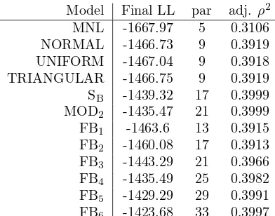
We first look at the achieved likelihoods of the various estimated structures, with a summary given in Table 2. As expected, all mixture models offer signifi-cant improvements in model fit over the MNL model, highlighting the presence of significant levels of taste heterogeneity relative to the linear specification of indirect utility. Here, for the more basic specifications, the performance with the Normal, Uniform and symmetrical Triangular distributions is very similar, with better performance being obtained with the more flexible SB distribution.
Moving on to the MOD and FB models, we can see that, whileM OD2obtains a better log-likelihood than the model using the SB distribution, the additional parameters mean that in terms of adjustedρ2
, the performance of the two mod-els is virtually identical. For the FB modmod-els, the adjusted ρ2
is always below that of the M OD2 model and the SB model, but there is a gradual and signifi-cant improvement in model fit as we increase the number of terms in the series expansions.
We proceed with a graphical analysis of the implied distributions resulting from the various models. As we are looking at the shapes of the estimated distri-butions this is much more informative than looking at the estimated parameters. Here, Figure 10 shows the CDF for βTT in the various models, with Figure 11 looking atβTC, Figure12looking at βHWand Figure13looking at βCH. In each case, the presentation of the FB results is limited to FB3, FB5 and FB6.
this is a true feature of the distribution of preferences in the population. There is a possibility that a distribution of a coefficient may indeed have multiple modes in a sample population in the case where there exists some segmentation of this population that is not accounted for in the model. However, for the number of modes to be exactly two11
across all four coefficients seems most unlikely. We can think of two potential explanations. The first potential explanation is that the effect is an artefact of the stated preference design. If this is true, then we are in effect measuring the design and not only the preferences which are the object of interest. It would then be prudent to seek to improve the design. The other potential explanation is that we are seeing a reference point effect (De Borger and Fosgerau, 2008), whereby the size of a parameter is influenced by whether the attribute being valued is larger or smaller than some reference. In any case, it is a real advantage of the flexible approaches that they allow such issues to be discovered. The potential problems here would have been invisible with the standard approaches.
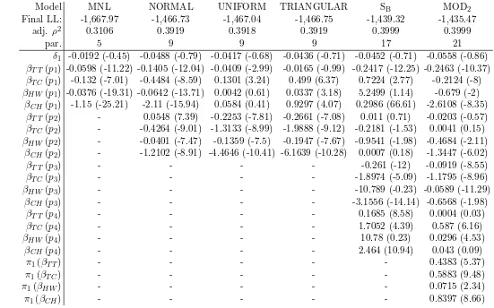
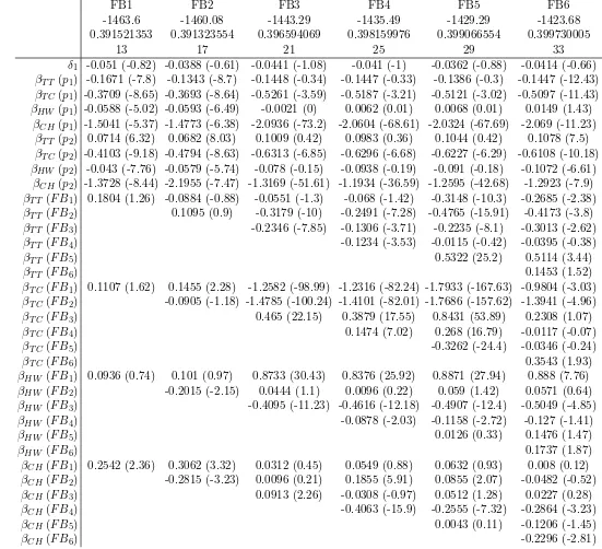
For completeness, the estimated parameters are presented in Table 3 for the standard models and the MOD2 while Table4 presents the estimates for the FB models. Here, δ1 is constant; the p1 parameters are used as fixed parameters in MNL, the mean in Normal, boundary to one side for Uniform and Triangular (this turns out to be the right hand boundary), the mean of underlying Normal in SB and the mean of the first Normal in MOD2. The p2 parameters are used as standard deviations for the Normal, interval width for the Uniform and Tri-angular, standard deviation of the underlying Normal for SB and std.dev. of the first Normal for MOD2. Thep3 parameters give the left boundary for the SBand the mean for the second Normal in MOD2. Finally, the p4 parameters give the interval width for the SB and the std.dev. for the second Normal in MOD2 and theπ parameters give the mass for the first Normal in MOD2. In the FB results presented in Table 4, the δ, β(p1) and β(p2) parameters are the same as in the Normal model in Table 3. The β(F B) parameters are the terms in the series expansions of the distributions for each coefficient.
On the estimated parameters we note in particular the low standard deviations (p2 and p4 parameters) for the MOD2 model, corresponding to almost point masses. On the FB models we note that most of the terms in the series expansion are quite significant in t-tests, with the exception of the last FB6 model.
11While the SBand MOD2 models are restricted to two modes, models FB3 to FB6 allow for
5
Conclusions
This paper has reported the findings of a systematic study using Monte Carlo experiments aimed at comparing the performance of various methods in retrieving random taste heterogeneity in a discrete choice context. Specifically, the analysis has compared the performance of four commonly used continuous distribution functions, the Normal, symmetrical Triangular, Uniform and Johnson SB, to that of two more advanced approaches discussed in this paper. The first of these two approaches, the FB approach, improves on the flexibility of a base distribution by adding in a series approximation using here Legendre polynomials, where the Normal distribution was chosen as the base. The second approach, the MOD approach, uses a discrete mixture of continuous distributions, where again, in the present study, the base distributions are all Normal.
The simulation study compared the performance of the six resulting models across seven separate case studies, making use of different assumptions for the true distribution of the single random parameter in the model. In each case study, fifty random versions of the data were generated to allow us to gauge the stability of the various approaches. We find as expected that the ability to reproduce an underlying true distribution depends on the number of parameters in the estimated distribution. The most flexible distributions are able to approximate a variety of different shapes and they result in higher log-likelihoods. Good performance was also obtained by the models using the Johnson SBdistribution. The latter has, however, the drawback that it cannot be made more flexible. So even though the Johnson SB distribution may do well in a particular application it is not possible to assess whether it does well enough. In contrast, one may just increase the number of parameters in the two flexible approaches and use a likelihood ratio test to decide when the number of parameters is sufficient.
The performance of the two-parameter distributions is poor in comparison. Even though this could be expected, we consider it illuminating to illustrate how these distributions fail and compare this to the application of more flexible dis-tributions. Many past applications of the Mixed Logit model have relied on such two-parameter distributions. On the other hand, the two advanced approaches discussed in this paper seem to perform very well across all the cases studied here, suggesting that they can approximate well a variety of distributions, ranging from the most trivial (Uniform) to more complex multi-modal distributions.
have somewhat higher variance than the FB estimates.
For non-smooth distributions, the MOD approach has the ability to become degenerate and have a point mass. The FB approach does not allow for point masses. This may be viewed as an advantage of the MOD approach if one believes in mass-points, a concept that, in an applied discrete choice context, only really makes sense for a mass-point at zero. However, this degeneracy is also a problem for the ability of the estimator to approximate smooth distributions and the estimator must be constrained in some way (cf. Coppejans, 2001). It may be conjectured that the higher variance of the MOD approach is related to this degeneracy problem.
In our application using the Swiss value of time data we have demonstrated that the flexible approaches are practical for real data. We found that all four coefficients tended to have bimodal distributions. This is something that deserves an explanation and we have put forward two potential explanations. The contri-bution of the flexible approaches that is relevant for the current paper is that they were able to reveal these features of the data that the less flexible approaches did not detect. The Johnson SB distribution and the MOD did have problems with degeneracy and it was not computationally possible to increase the MOD beyond MOD2. It is a possibility that this problem is related to weak identification of the distributions in the data. The FB approach did not have problems of degeneracy and there were no computational problems involved in increasing the number of parameters in the series expansions.
The flexibility of either of the two approaches can be increased by estimating additional parameters, in terms of additional terms in the series expansion in the FB approach, or additional distributions in the MOD approach. Here, an important advantage of the FB approach is that it is possible to add just one parameter at a time, while, with the MOD approach, it is necessary to add three parameters at the same time (location, variance and mass). Increasing the number of parameters inevitably leads to increased estimation cost, and issues of convergence to local maxima become more prominent.
Both approaches are not restricted to being based on the Normal distribution, but can use any continuous distribution as the base. Both approaches are also relatively easy to implement, where the FB approach has already been imple-mented in BIOGEME (Bierlaire,2003), and where estimation code for the MOD approach is available from the second author on request.
choice of an appropriate model. In one of the case studies in the simulation study discussed in this paper, one would, for example, be able to reveal that the lognor-mal distribution was an appropriate choice without imposing that distribution initially.
In a direct comparison of the two advanced approaches discussed in this paper, we can conclude that they are very similar in their ability to approximate smooth distributions. In general there is no reason to suppose that one approach should be better than the other, since both are able to approximate any distribution arbitrarily well by increasing the number of parameters. Our application to real data did however show that the MOD approach encountered some problems, where these problems may however be related to the data and not the MOD approach itself.
An important avenue for further research is the development and testing of the two approaches in more complex scenarios, such as in the presence of multiple random coefficients with potential correlation between them. This issue is related to the issue of the degree of model complexity that data will allow. There is clearly a limit in sight where normal-sized datasets will not allow us to identify all we would like to know about heterogenous preferences.
Acknowledgements
Part of the work described in this paper was carried out during a guest stay by Stephane Hess at the Institute of Transport and Logistics Studies at the University of Sydney. Financial support for Mogens Fosgerau from the Danish Social Science Research Council is acknowledged. The authors would like to thank Aruna Sivakumar and Katrine Hjort for comments on an earlier version of this paper.
References
Abay, G., Axhausen, K. W., 2001. Zeitkostenans¨atze im Personenverkehr: Vorstudie. SVI Forschungsauftrag 42/00, Schriftenreihe 472. Bundesamt f¨ur Strassen, UVEK, Bern. Bierens, H. J., 2007. Semi-nonparametric interval-censored mixed proportional hazard
models: Identification and consistency results. Econometric Theory Forthcoming. Bierlaire, M., 2003. BIOGEME: a free package for the estimation of discrete choice
models. Proceedings of the 3rd
Swiss Transport Research Conference, Monte Verit`a, Ascona.
Chen, X., 2006. Large sample sieve estimation of semi-nonparametric models. In: Hand-book of Econometrics, forthcoming Edition.
savings from a six-week diary. Transportation Research Part A: Policy and Practice 40 (5), 444–457.
Coppejans, M., 2001. Estimation of the binary response model using a mixture of distri-butions estimator (mod). Journal of Econometrics 102 (2), 231–269.
De Borger, B., Fosgerau, M., 2008. The trade-off between money and travel time: a test of the theory of reference-dependent preferences. Journal of Urban Economics Forthcoming.
Doornik, J. A., 2001. Ox: An Object-Oriented Matrix Language. Timberlake Consultants Press, London.
Fosgerau, M., 2006. Investigating the distribution of the value of travel time savings. Transportation Research Part B: Methodological 40 (8), 688–707.
Fosgerau, M., Bierlaire, M., 2007. A practical test for the choice of mixing distribution in discrete choice models. Transportation Research Part B: Methodological 41 (7), 784–794.
Fosgerau, M., Nielsen, S. F., 2006. Deconvoluting preferences and errors: a semi-nonparametric model for binomial data. Econometric Society European Meeting 2006. Gallant, A. R., Nychka, D. W., 1987. Semi-nonparametric maximum likelihood
estima-tion. Econometrica 55 (2), 363–390.
Geweke, J., Keane, M., 2001. Computationally intensive methods for integration in econo-metrics. In: Heckman, J. L., Leamer, E. (Eds.), Handbook of Econoecono-metrics. Elsevier, Amsterdam, Ch. 56, pp. 3463–3568.
Hensher, D. A., 2006. Reducing Sign Violation for VTTS Distributions through Recog-nition of an Individual’s Attribute Processing Strategy. ITLS working paper. Institute of Transport and Logistics Studies, University of Sydney.
Hensher, D. A., Greene, W. H., 2003. The Mixed Logit Model: The State of Practice. Transportation 30 (2), 133–176.
Hess, S., Axhausen, K. W., Polak, J. W., 2006. Distributional assumptions in Mixed Logit modelling. paper presented at the 85th
Annual Meeting of the Transportation Research Board, Washington, DC.
Hess, S., Bierlaire, M., Polak, J. W., 2005. Estimation of value of travel-time savings using mixed logit models. Transportation Research Part A: Policy and Practice 39 (2-3), 221–236.
Hess, S., Bierlaire, M., Polak, J. W., 2007. A systematic comparison of continuous and discrete mixture models. European Transport 36.
Klein, R. W., Spady, R. H., 1993. An efficient semiparametric estimator for binary re-sponse models. Econometrica 61 (2), 387–421.
McFadden, D., Train, K., 2000. Mixed MNL Models for discrete response. Journal of Applied Econometrics 15, 447–470.
Revelt, D., Train, K., 1998. Mixed Logit with repeated choices: households’ choices of appliance efficiency level. Review of Economics and Statistics 80 (4), 647–657. Train, K., 1998. Recreation demand models with taste differences over people. Land
Economics 74, 185–194.
Data MNL M(N) M(SB) M(T) M(MOD) M(U) M(FB) 5th
perc. -4707.76 -3708.26 -3565.42 -3697.21 -3565.34 -3644.74 -3579.57 mean -4643.54 -3642.45 -3497.32 -3633.74 -3497.10 -3583.83 -3515.96 DM(2)
95th
perc. -4575.35 -3567.01 -3428.72 -3558.48 -3428.74 -3510.46 -3444.96 5th
perc. -4456.99 -3866.13 -3846.47 -3860.49 -3845.40 -3849.76 -3845.82 mean -4380.80 -3798.70 -3781.05 -3793.08 -3779.00 -3782.95 -3779.66 DM(3)
95th
perc. -4313.91 -3741.58 -3723.33 -3736.87 -3722.72 -3725.52 -3722.66 5th
perc. -4263.78 -3860.01 -3781.90 -3874.35 -3782.62 -3897.44 -3784.43 mean -4165.97 -3792.01 -3713.90 -3805.26 -3716.43 -3827.84 -3718.88 LN
95th
perc. -4077.56 -3720.00 -3650.01 -3729.76 -3651.23 -3749.12 -3652.85 5th
perc. -4555.32 -3821.56 -3821.31 -3822.62 -3821.56 -3834.73 -3820.58 mean -4495.58 -3767.88 -3767.63 -3768.38 -3766.50 -3778.44 -3766.68 N
95th
perc. -4444.89 -3713.47 -3713.51 -3714.31 -3712.40 -3722.20 -3712.29 5th
perc. -4078.98 -3537.69 -3525.39 -3534.45 -3522.67 -3531.87 -3522.63 mean -3990.94 -3456.36 -3446.07 -3455.45 -3442.26 -3454.97 -3442.83 NM
95th
perc. -3904.82 -3370.11 -3363.78 -3368.02 -3361.03 -3370.84 -3360.67 5th
perc. -4748.22 -3698.21 -3669.81 -3692.69 -3669.53 -3672.41 -3669.80 mean -4687.77 -3616.24 -3584.53 -3611.91 -3583.00 -3591.84 -3583.47 2N
95th
perc. -4616.72 -3542.69 -3505.81 -3538.92 -3503.21 -3516.07 -3503.19 5th
perc. -4170.72 -3936.54 -3935.41 -3937.16 -3935.38 -3939.82 -3935.76 mean -4088.26 -3855.56 -3850.91 -3853.54 -3850.60 -3851.85 -3850.78 U
95th
[image:22.612.172.613.173.440.2]perc. -4025.88 -3778.32 -3776.16 -3776.89 -3775.04 -3776.54 -3775.61
Table 1: Model fit statistics across datasets and models
Model Final LL par adj. ρ2 MNL -1667.97 5 0.3106 NORMAL -1466.73 9 0.3919 UNIFORM -1467.04 9 0.3918 TRIANGULAR -1466.75 9 0.3919 SB -1439.32 17 0.3999 MOD2 -1435.47 21 0.3999 FB1 -1463.6 13 0.3915 FB2 -1460.08 17 0.3913 FB3 -1443.29 21 0.3966 FB4 -1435.49 25 0.3982 FB5 -1429.29 29 0.3991 FB6 -1423.68 33 0.3997
Model MNL NORMAL UNIFORM TRIANGULAR SB MOD2
Final LL: -1,667.97 -1,466.73 -1,467.04 -1,466.75 -1,439.32 -1,435.47
adj. ρ2
0.3106 0.3919 0.3918 0.3919 0.3999 0.3999
par. 5 9 9 9 17 21
δ1 -0.0192 (-0.45) -0.0488 (-0.79) -0.0417 (-0.68) -0.0436 (-0.71) -0.0452 (-0.71) -0.0558 (-0.86) βT T(p1) -0.0598 (-11.22) -0.1405 (-12.04) -0.0409 (-2.99) -0.0165 (-0.99) -0.2417 (-12.25) -0.2463 (-10.37) βT C(p1) -0.132 (-7.01) -0.4484 (-8.59) 0.1301 (3.24) 0.499 (6.37) 0.7224 (2.77) -0.2124 (-8) βHW (p1) -0.0376 (-19.31) -0.0642 (-13.71) 0.0042 (0.61) 0.0337 (3.18) 5.2499 (1.14) -0.679 (-2)
βCH(p1) -1.15 (-25.21) -2.11 (-15.94) 0.0584 (0.41) 0.9297 (4.07) 0.2986 (66.61) -2.6108 (-8.35) βT T(p2) - 0.0548 (7.39) -0.2253 (-7.81) -0.2661 (-7.08) 0.011 (0.71) -0.0203 (-0.57) βT C(p2) - -0.4264 (-9.01) -1.3133 (-8.99) -1.9888 (-9.12) -0.2181 (-1.53) 0.0041 (0.15) βHW (p2) - -0.0401 (-7.47) -0.1359 (-7.5) -0.1947 (-7.67) -0.9541 (-1.98) -0.4684 (-2.11)
βCH(p2) - -1.2102 (-8.91) -4.4646 (-10.41) -6.1639 (-10.28) 0.0007 (0.18) -1.3447 (-6.02)
βT T(p3) - - - - -0.261 (-12) -0.0919 (-8.55)
βT C(p3) - - - - -1.8974 (-5.09) -1.1795 (-8.96)
βHW (p3) - - - - -10.789 (-0.23) -0.0589 (-11.29)
βCH(p3) - - - - -3.1556 (-14.14) -0.6568 (-1.98)
βT T(p4) - - - - 0.1685 (8.58) 0.0004 (0.03)
βT C(p4) - - - - 1.7052 (4.39) 0.587 (6.16)
βHW (p4) - - - - 10.78 (0.23) 0.0296 (4.53)
βCH(p4) - - - - 2.464 (10.94) 0.043 (0.09)
π1(βT T) - - - 0.4383 (5.37)
π1(βT C) - - - 0.5883 (9.48)
π1(βHW) - - - 0.0715 (2.34)
[image:24.612.107.658.132.476.2]π1(βCH) - - - 0.8397 (8.66)
Table 3: Model estimation on Swiss route choice data (part 1, asy. t-ratios in brackets)
FB1 FB2 FB3 FB4 FB5 FB6
-1463.6 -1460.08 -1443.29 -1435.49 -1429.29 -1423.68
0.391521353 0.391323554 0.396594069 0.398159976 0.399066554 0.399730005
13 17 21 25 29 33
δ1 -0.051 (-0.82) -0.0388 (-0.61) -0.0441 (-1.08) -0.041 (-1) -0.0362 (-0.88) -0.0414 (-0.66) βT T(p1) -0.1671 (-7.8) -0.1343 (-8.7) -0.1448 (-0.34) -0.1447 (-0.33) -0.1386 (-0.3) -0.1447 (-12.43) βT C(p1) -0.3709 (-8.65) -0.3693 (-8.64) -0.5261 (-3.59) -0.5187 (-3.21) -0.5121 (-3.02) -0.5097 (-11.43) βHW(p1) -0.0588 (-5.02) -0.0593 (-6.49) -0.0021 (0) 0.0062 (0.01) 0.0068 (0.01) 0.0149 (1.43)
βCH(p1) -1.5041 (-5.37) -1.4773 (-6.38) -2.0936 (-73.2) -2.0604 (-68.61) -2.0324 (-67.69) -2.069 (-11.23) βT T(p2) 0.0714 (6.32) 0.0682 (8.03) 0.1009 (0.42) 0.0983 (0.36) 0.1044 (0.42) 0.1078 (7.5) βT C(p2) -0.4103 (-9.18) -0.4794 (-8.63) -0.6313 (-6.85) -0.6296 (-6.68) -0.6227 (-6.29) -0.6108 (-10.18) βHW(p2) -0.043 (-7.76) -0.0579 (-5.74) -0.078 (-0.15) -0.0938 (-0.19) -0.091 (-0.18) -0.1072 (-6.61)
βCH(p2) -1.3728 (-8.44) -2.1955 (-7.47) -1.3169 (-51.61) -1.1934 (-36.59) -1.2595 (-42.68) -1.2923 (-7.9) βT T(F B1) 0.1804 (1.26) -0.0884 (-0.88) -0.0551 (-1.3) -0.068 (-1.42) -0.3148 (-10.3) -0.2685 (-2.38) βT T(F B2) 0.1095 (0.9) -0.3179 (-10) -0.2491 (-7.28) -0.4765 (-15.91) -0.4173 (-3.8)
βT T(F B3) -0.2346 (-7.85) -0.1306 (-3.71) -0.2235 (-8.1) -0.3013 (-2.62)
βT T(F B4) -0.1234 (-3.53) -0.0115 (-0.42) -0.0395 (-0.38)
βT T(F B5) 0.5322 (25.2) 0.5114 (3.44)
βT T(F B6) 0.1453 (1.52)
βT C(F B1) 0.1107 (1.62) 0.1455 (2.28) -1.2582 (-98.99) -1.2316 (-82.24) -1.7933 (-167.63) -0.9804 (-3.03) βT C(F B2) -0.0905 (-1.18) -1.4785 (-100.24) -1.4101 (-82.01) -1.7686 (-157.62) -1.3941 (-4.96)
βT C(F B3) 0.465 (22.15) 0.3879 (17.55) 0.8431 (53.89) 0.2308 (1.07)
βT C(F B4) 0.1474 (7.02) 0.268 (16.79) -0.0117 (-0.07)
βT C(F B5) -0.3262 (-24.4) -0.0346 (-0.24)
βT C(F B6) 0.3543 (1.93)
βHW(F B1) 0.0936 (0.74) 0.101 (0.97) 0.8733 (30.43) 0.8376 (25.92) 0.8871 (27.94) 0.888 (7.76) βHW(F B2) -0.2015 (-2.15) 0.0444 (1.1) 0.0096 (0.22) 0.059 (1.42) 0.0571 (0.64)
βHW(F B3) -0.4095 (-11.23) -0.4616 (-12.18) -0.4907 (-12.4) -0.5049 (-4.85)
βHW(F B4) -0.0878 (-2.03) -0.1158 (-2.72) -0.127 (-1.41)
βHW(F B5) 0.0126 (0.33) 0.1476 (1.47)
βHW(F B6) 0.1737 (1.87)
βCH(F B1) 0.2542 (2.36) 0.3062 (3.32) 0.0312 (0.45) 0.0549 (0.88) 0.0632 (0.93) 0.008 (0.12) βCH(F B2) -0.2815 (-3.23) 0.0096 (0.21) 0.1855 (5.91) 0.0855 (2.07) -0.0482 (-0.52)
βCH(F B3) 0.0913 (2.26) -0.0308 (-0.97) 0.0512 (1.28) 0.0227 (0.28)
βCH(F B4) -0.4063 (-15.9) -0.2555 (-7.32) -0.2864 (-3.23)
βCH(F B5) 0.0043 (0.11) -0.1206 (-1.45)
βCH(F B6) -0.2296 (-2.81)
[image:25.612.110.661.54.556.2]γ γ γ
γ γ γ
[image:26.612.129.529.151.661.2]γ γ γ
= σ = = − σ =
π = π = π = π =
= − σ = = π =
σ = σ = σ = σ =
= − = σ = σ π =
σ = σ = σ = σ =
= − σ = σ = π =
[image:27.612.100.677.150.454.2]= = = = −
Figure 2: CDF plots for various mixtures of two Normal distributions
α
(
α
)
α
(
α
)
α
(
α
)
α
(
α
)
α
(
α
)
α
(
α
[image:28.612.112.677.152.457.2])
Figure 3: CDF plots forα in models estimated on DM(2) data
α
(
α
)
α
(
α
)
α
(
α
)
α
(
α
)
α
(
α
)
α
(
α
[image:29.612.114.677.151.457.2])
Figure 4: CDF plots forα in models estimated on DM(3) data
α
(
α
)
α
(
α
)
α
(
α
)
α
(
α
)
α
(
α
)
α
(
α
[image:30.612.110.676.152.457.2])
Figure 5: CDF plots forα in models estimated on LN data
α
(
α
)
α
(
α
)
α
(
α
)
α
(
α
)
α
(
α
)
α
(
α
[image:31.612.112.677.152.457.2])
Figure 6: CDF plots forα in models estimated on N data
α
(
α
)
α
(
α
)
α
(
α
)
α
(
α
)
α
(
α
)
α
(
α
[image:32.612.111.679.152.456.2])
Figure 7: CDF plots forα in models estimated on NM data
α
(
α
)
α
(
α
)
α
(
α
)
α
(
α
)
α
(
α
)
α
(
α
[image:33.612.113.677.152.457.2])
Figure 8: CDF plots forα in models estimated on 2N data
α
(
α
)
α
(
α
)
α
(
α
)
α
(
α
)
α
(
α
)
α
(
α
[image:34.612.117.676.150.458.2])
Figure 9: CDF plots forα in models estimated on U data
β
β
β
β
β
β
β
β
β
β
β
β
β
β
β
[image:35.612.129.514.143.359.2]β
Figure 10: CDF plots forβTT in models estimated on Swiss route choice data
β
β
β
β
β
β
β
β
β
β
β
β
β
β
β
β
[image:35.612.128.512.418.637.2]β
β
β
β
β
β
β
β
β
β
β
β
β
β
β
[image:36.612.128.515.144.360.2]β
Figure 12: CDF plots forβHW in models estimated on Swiss route choice data
β
β
β
β
β
β
β
β
β
β
β
β
β
β
β
β
[image:36.612.128.513.418.637.2]