Parameterization of contrails in the UK Met Office Climate Model

Model

_.

White Rose Research Online URL for this paper:

http://eprints.whiterose.ac.uk/76988/

Article:

Rap, A, Forster, PM, Jones, A et al. (4 more authors) (2010) Parameterization of contrails

in the UK Met Office Climate Model. Journal of Geophysical Research Atmospheres, 115

(D10). D10205. ISSN 0148-0227

https://doi.org/10.1029/2009JD012443

[email protected] https://eprints.whiterose.ac.uk/

Reuse

Unless indicated otherwise, fulltext items are protected by copyright with all rights reserved. The copyright exception in section 29 of the Copyright, Designs and Patents Act 1988 allows the making of a single copy solely for the purpose of non-commercial research or private study within the limits of fair dealing. The publisher or other rights-holder may allow further reproduction and re-use of this version - refer to the White Rose Research Online record for this item. Where records identify the publisher as the copyright holder, users can verify any specific terms of use on the publisher’s website.

Takedown

If you consider content in White Rose Research Online to be in breach of UK law, please notify us by

Here

for

Full Article

Parameterization of contrails in the UK Met Office

Climate Model

A. Rap,

P. M. Forster,

A. Jones,

O. Boucher,

J. M. Haywood,

N. Bellouin,

and R. R. De Leon

Received 7 May 2009; revised 7 December 2009; accepted 24 December 2009; published 19 May 2010.

[1]

Persistent contrails are believed to currently have a relatively small but significant

positive radiative forcing on climate. With air travel predicted to continue its rapid growth

over the coming years, the contrail warming effect on climate is expected to increase.

Nevertheless, there remains a high level of uncertainty in the current estimates of contrail

radiative forcing. Contrail formation depends mostly on the aircraft flying in cold and

moist enough air masses. Most studies to date have relied on simple parameterizations

using averaged meteorological conditions. In this paper we take into account the

short

_‐

term variability in background cloudiness by developing an on

_‐

line contrail

parameterization for the UK Met Office climate model. With this parameterization, we

estimate that for the air traffic of year 2002 the global mean annual linear contrail coverage

was approximately 0.11%. Assuming a global mean contrail optical depth of 0.2 or smaller

and assuming hexagonal ice crystals, the corresponding contrail radiative forcing was

calculated to be less than 10 mW m

in all

‐

sky conditions. We find that the natural cloud

masking effect on contrails may be significantly higher than previously believed. This new

result is explained by the fact that contrails seem to preferentially form in cloudy

conditions, which ameliorates their overall climate impact by approximately 40%.

Citation: Rap, A., P. M. Forster, A. Jones, O. Boucher, J. M. Haywood, N. Bellouin, and R. R. De Leon (2010),

Parameterization of contrails in the UK Met Office Climate Model,J. Geophys. Res.,115, D10205, doi:10.1029/2009JD012443.

1.

Introduction

[2] Condensation trails, or simply contrails, are visible

line‐shaped high clouds that form behind an aircraft. As with all clouds, their presence causes an alteration in the Earth’s radiation budget, via their shortwave (SW) albedo effect, i.e., they reduce the amount of SW radiation reaching the Earth, and their longwave (LW) greenhouse effect; that is, they reduce the amount of LW radiation leaving Earth to space. The balance between these two competing effects is strongly dependent on the cloud optical properties and altitude (temperature) [Fu et al., 2000]. While for all cloud cover in general, the cooling effect dominates the warming effect, the opposite has been shown to be the case for thin cirrus and contrails.

[3] The theory behind the contrail formation process is

well understood since the publication of the first two papers that provided the explanation of this process based on thermodynamic theory, namely those bySchmidt[1941] and

Appleman [1953]. Nowadays it is therefore known that

contrails form under liquid water saturation conditions as a result of heat and water vapor mixing between the warm and moist exhaust and the cool ambient air. When they form in dry unsaturated air, contrails are usually short‐lived, but when the ambient relative humidity exceeds ice saturation, they persist and can develop into extended cirrus cloud layers [see, e.g., Schumann, 1996]. Existing studies have shown that for these persistent contrails, their daily average LW radiative forcing (RF) effect is larger than their SW effect, meaning that contrails cause a positive net RF, and therefore a warming [see, e.g.,Meerkötter et al., 1999]. The magnitude of this net positive RF estimated by various studies for the air traffic of the year 1985, varies from a value of 2.0 mW m−2_{[Stuber and Forster, 2007] to a value} of 17 mW m−2 _{[Minnis et al., 1999]. According to the} Intergovernmental Panel on Climate Change (IPCC) fourth assessment [Forster et al., 2007], the linear contrail radia-tive forcing for the year 2005 is estimated at 10 mW m−2_, with an uncertainty factor of 3 caused by a low level of current scientific understanding. This represents an impor-tant contribution, i.e., approximately 20%, of the total avi-ation RF. The high uncertainty factor still present in our estimates of contrail RF is mainly due to the limited knowledge of contrail optical properties and contrail cov-erages. When estimating global contrail RF, most available models assume constant optical properties for contrails. Currently there are only two climate model approaches that 1

Institute for Climate and Atmospheric Science, School of Earth and Environment, University of Leeds, Leeds, UK.

2

Met Office Hadley Centre, Exeter, UK.

3_{Centre for Air Transport and the Environment, Manchester}

Metropolitan University, Manchester, UK.

have the ability of considering a geographical and temporal variability for contrail optical depths, namely thePonater et al.[2002] model, with amendments byMarquart and Mayer

[2002], and the Burkhardt and Kärcher [2009] contrail cirrus model, both hosted by the ECHAM4 climate model. As air traffic is expected to experience a significant increase in the future, the contrail warming effect may become stronger and therefore the development of more reliable models that can accurately estimate contrail formation and their radiative impact is considered important. Also, more than one GCM configuration is desirable to provide reliable error estimates, due to the different performance of cirrus parameterizations in GCMs, as indicated by, for example,

Lohmann and Kärcher [2002] andWaliser et al.[2009]. [4] The aim of the current study is to develop a new linear

contrail parameterization by adapting the contrail parame-terization from Ponater et al.[2002] to the second version of the UK Hadley Centre Global Environmental Model (HadGEM2) [Collins et al., 2008]. This provides the research community with an additional GCM tool for esti-mating the impact of contrails on the Earth’s radiative budget and climate, and an alternative development platform for advanced research on the global impact of aircraft induced cloudiness. This paper addresses only the radiative forcing aspects of the parameterization. In a planned follow‐

up paper the full climate impact of these parameterized contrails will be evaluated.

[5] Section 2 of the present paper describes the

method-ology of our contrail parameterization. The results obtained for the contrail coverage, optical depth, and radiative forcing are then presented in sections 3, 4, and 5, respectively. Finally, section 6 discusses some of the main results and summarizes the conclusions of this study.

2.

Contrail Parameterization Within HadGEM2

[6] This section describes the implementation of the

contrail parameterization within the Hadley Centre climate model HadGEM2. Section 2.1 briefly presents the host climate model, section 2.2 describes the details of our parameterization and section 2.3 shows some benchmark calculations for the evaluation of the radiation code employed in this study.

2.1. Host Climate Model: HadGEM2

[7] The host climate model for our contrail

parameteri-zation is the Hadley Centre climate model HadGEM2 [Collins et al., 2008]. The model generates its own meteo-rology based on greenhouse gases, aerosol emissions and land use distribution for the year 2000. The sea surface temperatures and sea ice are from the AMIP II observed climatology [Hurrell et al., 2008], averaged over the 1978–

1995 period.

[8] The radiation scheme of HadGEM2 is that ofEdwards and Slingo [1996], which will be described in section 2.3. The cloud scheme within HadGEM2 is the same with the one from HadGEM1 [seeMartin et al., 2006]. This is based on theSmith[1990] scheme, in which cloud water and cloud amount are diagnosed from total moisture and liquid water potential temperature using a triangular probability distri-bution function. Also, the main assumption regarding the

interaction with radiation and clouds in the model is that clouds consist of four components (stratiform water and ice, convective water and ice) and they are treated as plane parallel (no 3D effects) with a maximum random overlap assumption.

[9] The HadGEM2 experiments employ a resolution

configuration of 192 (longitude) × 145 (latitude) × 38 (altitude). This differs from the resolution of the off‐line radiation code calculations employed in sections 2.3 and 5.1.

2.2. Contrail Parameterization

[10] For the contrail parameterization within HadGEM2

we adopt a similar methodology to the one developed by

Ponater et al. [2002] for the ECHAM4 climate model. Based on contrail formation thermodynamics, the maximum temperature and minimum relative humidity thresholds necessary for contrails to form depend only on the ambient temperature, pressure and relative humidity, as well as on the emission index of water vapor, the specific heat of fuel combustion and on the propulsion efficiency of the aircraft engine.

[11] The threshold temperature (in K) for contrail

forma-tion used in our parameterizaforma-tion is the one estimated by

Schumann[1996], namely

Tcontr¼226:69þ9:43 lnðG 0:053Þ þ0:72 ln2ðG 0:053Þ;

ð1Þ

where G is the slope of the mean phase trajectory in the turbulent exhaust field on an absolute temperature versus water vapor partial pressure diagram. G has the unit of Pa K−1_{and is given by}

G¼ EIH2Ocpp

Qð1 Þ; ð2Þ

where EIH₂O= 1.25 is the emission index of water vapor, cp= 1004 J kg−1_K−1_{is the isobaric heat capacity of air,pis} the ambient air pressure,= 0.622 is the ratio of molecular masses of water and dry air,Q= 43 MJ kg−1_{is the specific} combustion heat, and h = 0.3 is the average propulsion efficiency of the jet engine.

[12] The critical relative humidity, rcontr, for contrail

formation at a given ambient temperature T can then be calculated as

rcontrð Þ ¼T

G Tð TcontrÞ þeliqsatðTcontrÞ

eliq_{satð Þ}T ; ð3Þ

whereesat liq

(T) is the saturation pressure of water vapor with respect to the liquid phase, at a given temperatureT.

[13] As in the Ponater et al. [2002] study, in order to

adapt the theory of local contrail formation to the HadGEM2 cloud scheme, we define a modified relative humidity thresholdr*crit, by combining the theoretical threshold rcontr

with the threshold rcrit = 0.8 controlling the initiation of

cirrus formation in HadGEM2,

r*_crit¼rcontrrcrit: ð4Þ

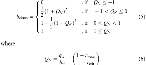
[14] FollowingSmith[1990], the UK Met Office Climate

on the assumption of a symmetric triangular probability distribution function (PDF) of the total water saturation excess, s, around its grid box mean. Details are given by

Wilson and Gregory [2003] and Wilson [2007]. Using the

Smith[1990] cloud fraction formula, the natural cirrus cloud coverage (bcirrus) is then given by

bcirrus¼

0 ;if QN 1

1

2ð1þQNÞ

2 _{;if 1<Q}

N 0

1 1

2ð1 QNÞ 2

;if 0<QN <1

1 ;if 1QN

8 > > > > < > > > > :

; _ð5_Þ

where

QN ¼ qcf bsi

1 rwater 1 rcrit

; _ð6Þ

with qcf being the ice water content and bsi = (1 − rcrit) qsatwaterthe half width of the triangular PDF ins. This width

is defined such that the condensation in the grid box occurs when the grid box mean relative humidity over waterrwater= q/qsatwaterequals the prescribedrcrit.

[15] It should be noted here that the Smith [1990] ice

cloud scheme employs the saturation humidity with respect to water, and not with respected to ice. This was chosen primarily to produce consistency in cloud fractions when liquid water cloud was homogeneously frozen to ice [see

Wilson, 2007], and in our case means that equation (4) is consistent, all three relative humidities being defined over water.

[16] Employing r*crit from equation (4), but maintaining

the same width bsiof the triangular PDF, we define

Q*_N ¼qcf

bsi

1 rwater

1 r*_crit

!

: ð7Þ

As pointed out byBurkhardt et al.[2008], when developing a new coverage parameterization (in our case, linear contrail coverage), it is important to maintain consistency with the existing natural cloud coverage parameterization, by employing in both cases the same PDF of total water, with the same fixed width.

[17] With this newQ*N, we obtain a potential cloud

cover-age for all high clouds (btotalpotential), including both natural cirrus

and contrails, by replacingQNwithQ*_Nin equation (5). We can then define a potential cloud coverage for contrails only as

bpotential_contr ¼bpotential_total bcirrus: ð8Þ

[18] Figure 1 shows bcirrus,bcontrpotentialand btotalpotentialas

func-tions of the grid box mean relative humidity with respect to water for the case whenrcontr= 0.5 andrcrit= 0.8. It can be

seen that the potential contrail cover reaches its maximum at values comparatively larger than those fromPonater et al.

[2002] as shown in their Figure 1.

[19] The final parameterized contrail coverage is then

calculated using the following expression:

bcontr¼Dbpotentialcontr ; ð9Þ

where g is a nonphysical scaling factor obtained by cali-brating the temporal and spatial average of contrail coverage to observed conditions, and D is the local distance flown that allows us to account for the dependency of the contrail coverage on the density of air traffic. The contrail coverage parameterized in this way (bcontr) is a three‐dimensional

field, defined for every (longitude × latitude × altitude) grid box in the model.

[20] For the distance flown dataD, we use the AERO2K

global air traffic inventory [Eyers et al., 2004]. This inventory provides the total distance flown by aircraft on a three‐dimensional grid for each month of the year 2002. Also, for one week in June, the data is provided for four 6‐hourly time periods starting at midnight GMT. We apply this diurnal variation from that week in June to the distance flown for all months.

[21] It should also be mentioned that the parameterization

considers only contrails that persist for at least 30 minutes, i.e., one model time step. An implicit contrail persistence criterion is incorporated into the scheme using the same approach as that ofPonater et al.[2002]; that is, if there is no contrail ice water formation at some time step, then the contrail coverage is reset to zero.

[22] The contrail optical depth, t, is calculated as the

integral over vertical levels of the contrail specific extinction coefficient,kextin m2kg−1, weighted by the contrail mass‐

mixing ratio, MMR in kg kg−1_{, following:}

ð Þ ¼ Z

z

kextð ÞMMRð Þzð Þzdz; ð10Þ

where l is the wavelength, z is the vertical coordinate (in m), andris the air density (kg m−3_{). Specific extinction} coefficients are obtained using the contrail size distribution and optical properties ofStrauss et al. [1997]. Throughout this paper, the optical depth is assumed to be independent of

Figure 1. Parameterization of the fractional coverage of natural cirrus cloudsbcirrus(dashed line), potential contrails bcontrpotential(dotted line), and the sum of total natural cirrus and

contrailsbtotalpotential(solid line) in case ofrcontr= 0.5,rcrit= 0.8

wavelength and is given at 0.55 microns. Finally, it should be mentioned that the contrail mass‐mixing ratio MMR is a dimensionless variable defined as the product of the ice mass mixing ratio and the contrail fraction.

2.3. Benchmark Calculations

[23] Once contrail coverage and optical depth

distribu-tions are generated, these can then be used in order to evaluate the contrail RF by employing a radiative transfer model. The model used in this study is the Edwards‐Slingo radiation code [seeEdwards and Slingo, 1996], in both its off‐line and on‐line (within HadGEM2) versions. The cli-mate model based version of this code employs 6 bands in the shortwave and 9 bands in the longwave and adopts a delta‐Eddington 2 stream scattering solver at all wave-lengths. As noted by Marquart and Mayer [2002], not accounting for scattering by contrail in the longwave can be a source of error.

[24] In order to evaluate the performance of this radiation

code for estimating the contrail RF we first perform some test calculations where the contrail cover is represented by a homogeneous constant global cloud cover of cirrus. As in work by Meerkötter et al. [1999], a 100% homogeneous contrail coverage is assumed at 250 hPa, with a constant optical deptht= 0.52 at 0.55mm, an ice water content IWC = 21 mg m−3_{, and a generalized mean effective size Dge =} 23mm. FollowingFu[1996], the generalized mean effective size is given by

Dge¼

2 ffiffiffi 3 p

IWC 3iAc

; _ð11_Þ

whereri= 0.9167 g cm−3is the ice density andAcis the total

cross‐sectional area of the particle per unit volume. Also, the effective radius (re) is given by [seeFu, 1996]

re¼

3IWC

4iAc ð

12_Þ

and can therefore be related toDgein the form

re¼

3pffiffiffi3

8 Dge: ð13Þ

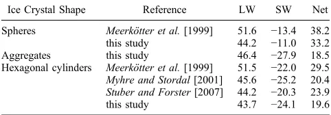
[25] Three different ice particle shapes are considered,

namely spheres, aggregates, and hexagonal cylinders. Using the off‐line Edwards‐Slingo code with the 144 (longitude) ×

72 (latitude) × 23 (altitude) resolution, the LW, SW and net RFs at the top of the atmosphere can be estimated. Table 1 shows the results obtained by the model for the global mean RFs, compared with similar cases presented byMeerkötter et al. [1999],Myhre and Stordal[2001], and Stuber and Forster [2007]. As already shown by these earlier studies, we note that the shape of the ice particles plays an important role, with aggregates and hexagonal cylinders exerting sig-nificantly less net RFs than spherical ice particles. This difference in the net RFs is mainly due to the different influences on the SW radiative flux, as the shape does not change the LW fluxes significantly. The choice of the ice particle shape is therefore an important factor in estimating the contrail RF. In the remainder of this paper we use hexagonal cylinders in all calculations. In terms of com-paring our model results with those presented in the other three publications, it can be seen that the RFs obtained by our Edwards‐Slingo code are broadly consistent with those reported by the other authors, although due to SW and LW forcing cancellation, net differences in forcing can be as large as 30%.

[26] Another test for the radiation code is performed by

considering the Myhre and Stordal [2001] case, also repeated by Stuber and Forster [2007], where a 1% homogeneous contrail coverage is assumed at 250 hPa, with an optical deptht = 0.3 at 0.55mm, an ice water content IWC = 21 mg m−3_{, and a generalized effective sizeDge=} 23mm. For these calculations, the natural clouds are based on monthly averaged distributions for the 1983–2002 period, for low‐level, midlevel and high‐level cloud from the International Satellite Cloud Climatology (ISCCP) project. For comparison, Stuber and Forster [2007] also used ISCCP data, whilstMyhre and Stordal[2001] employed 1996 natural clouds from the European Centre for Medium‐

Range Weather Forecasts (ECMWF) analysis.

[27] Table 2 shows the results obtained in this case, for

both clear‐sky and all‐sky conditions, which are remarkably similar to those reported by the above two papers. Both the LW and SW contrail RFs are reduced by the presence of clouds, via the cloud masking effect. However, since this effect has similar magnitudes in the LW and SW, this results in the clouds having a very small effect on the net contrail RFs.

[28] For purely technical reasons, on_‐line contrail RF

calculations within HadGEM2 are easier to perform if the contrail is artificially considered as a new aerosol species, rather than an ice cloud. The only shortcoming of such a technical assumption is that, for aerosols, the model does not have an“aerosol fraction”. Therefore, if we are to include contrails as aerosols in HadGEM2 RF calculations, then we

Table 1. Global Mean Radiative Forcing at the Top of the Atmosphere for a 100% Homogeneous Contrail Coverage at 250 hPa Indicating the Dependence of Ice Crystal Shapea

Ice Crystal Shape Reference LW SW Net

Spheres Meerkötter et al.[1999] 51.6 −13.4 38.2

this study 44.2 −11.0 33.2

Aggregates this study 46.4 −27.9 18.5

Hexagonal cylinders Meerkötter et al.[1999] 51.5 −22.0 29.5

Myhre and Stordal[2001] 45.6 −25.2 20.4

Stuber and Forster[2007] 44.2 −20.3 23.9

this study 43.7 −24.1 19.6

a

Unit is W m−2_{. Studies are for July values and for an optical depth of}

0.52 at 0.55mm and an ice water content of 21 mg/m3.

Table 2. Radiative Forcing at the Top of the Atmosphere for a 1% Homogeneous Contrail Coverage at 250 hPaa

Reference

Clear Sky All Sky

LW SW Net LW SW Net

Myhre and Stordal[2001] 0.27 −0.15 0.12 0.21 −0.09 0.12

Stuber and Forster[2007] 0.25 −0.12 0.13 0.19 −0.06 0.13

this study 0.27 −0.15 0.12 0.22 −0.10 0.12

a_{Unit is W m}−2_{. Studies are for July values, an optical depth of 0.3 at}

must be able to control the contrail coverage (cloud fraction) by another parameter, that is present in the aerosol radiative transfer scheme of the model. The best candidate for such a parameter is the aerosol optical depth. Thus, we want to check if, from a radiative transfer point of view, it is rea-sonable to assume that instead of having a bcontr contrail

coverage of optical depth t, we can assume of having a 100% contrail coverage of optical depthbcontrt. Technically,

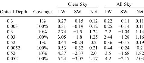
this would allow the treatment of the contrails as aerosols. We consider four such coupled cases: the first one with 1% contrail coverage andt= 0.3, compared with 100% contrail coverage and t = 0.003, and the second one for a 10% contrail coverage with t = 0.3, compared with 100% con-trail coverage and t = 0.03. The third and fourth cases consider similar coverages but optical depths of t = 0.52, t = 0.052 andt= 0.0052. Again, both clear‐sky and all‐sky conditions are investigated.

[29] The results presented in Table 3 show that when

considering a 100% contrail coverage, with a correspond-ingly smaller optical depth, the magnitude for both the LW and SW forcings increases, compared with the case when 1% or 10% contrail coverages are assumed but with higher optical depths. These differences would affect the forcing diurnal variations and may affect the climate response. However, for the net forcings, these differences virtually cancel each other, meaning that controlling the contrail fraction in the model by correspondingly altering the optical depth is not an unreasonable assumption for daily averaged forcing estimates. It should also be mentioned that when doing this scaling on the optical depth the other contrail optical properties remain unchanged.

3.

Contrail Coverage

[30] With the contrail parameterization described in

section 2.2 incorporated in the HadGEM2 GCM, a 5 year simulation was performed. The averaged contrail cover over these 5 years represents a fractional coverage within each model grid box for all contrails. Integrating the contrail coverage vertically for all model levels, using the random overlap principle, a two‐dimensional coverage distribution is obtained. However, this distribution needs to be calibrated using some available observations for contrail coverage, via the nonphysical scaling factorgfrom equation (9).

[31] The observations employed for calibration in this

study are those reported byBakan et al.[1994], which were also used in other studies such as those by Ponater et al.

[2002] and Rädel and Shine [2008]. These observations are 24 h means of visual inspection of quicklook photo-graphic prints from NOAA satellites infrared images for the geographical area of 30°W to 30°E and 35°N to 75°N (referred to here as the “Bakan”area). The Bakan et al.

[1994] study uses observations from two periods, namely 1979–1981 and 1989–1992, while the AERO2K traffic inventory we use in this paper corresponds to the year 2002. According toRädel and Shine[2008], a factor of 2 is a good approximation of the air traffic increase in the“Bakan”area from 1985 (the year considered representative for theBakan et al. [1994] observations) to 2002. This factor of 2 is therefore taken into account when scaling the contrail cov-erage produced by the parameterization to the observed average coverage for the“Bakan”area, which was 0.375% for the 1985 air traffic.

[32] For the calculation of the scaling factor g from

equation (9), we only consider the visible contrails, where the same criterion for visible contrails as in work byPonater et al. [2002] is used; that is, the contrails must have an optical depth larger than 0.02 and they must not be dis-guised by natural clouds (the natural clouds coverage in the layers above or immediately below must not be larger than 80%).

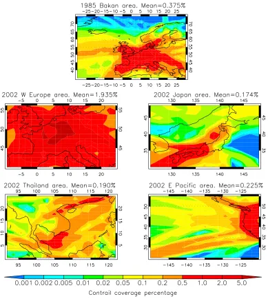
[33] Once the scaling factor is chosen, other observed

coverages reported by some existing studies for various geographical regions can be investigated (see Figure 2). One such a region is the western Europe area of 10°W to 23°E and 40°N to 56°N fromMeyer et al. [2002], where data of the Advanced Very High Resolution Radiometer (AVHRR) sensor onboard the NOAA 14 satellite was analyzed for the 1995–1997 period using an operational contrail detection algorithm. The 1985 average contrail coverage for this region reported byMeyer et al.[2002] is 0.5%, whileBakan et al.[1994] andStuber and Forster[2007] reported values of approximately 0.7% and 0.9%, respectively. Our value for the same region is 0.97% for the year 1985.

[34] For the eastern Pacific area of 120°W to 150°W and

25°N to 55°N the average contrail coverage during May, August and November 2002 and February 2003 reported by

Minnis et al.[2005] was 0.31%. Their calculation was based on 1 km window channel data from the AVHRR on the NOAA 16 satellite, that was analyzed using a automated detection method from Mannstein et al.[1999]. Using the AERO2K air traffic data, combined with ECMWF analysis,

Rädel and Shine [2008] found a 2002 mean contrail cov-erage for the same region of 0.27%, while the value found using our current study is 0.23%.

[35] Meyer et al.[2007] used remote sensing observations

from the NOAA/AVHRR satellite corresponding to the year 1998, analyzed by a fully automated contrail detection algorithm to produce contrail coverage for two regions covering Japan (125.625°E to 148.125°E and 29.689°N to 48.245°N) and Thailand (91.88°E to 121.875°E and 0°N to 25°N); for these two regions their observed coverages were 0.25% and 0.13%, respectively, while our parameterization generates coverages corresponding to the year 2002 of 0.17% and 0.19%, respectively.

[36] The range of regional estimates of contrail cover

shows variation in coverage of over 50% between different estimates and the lack of detailed coverage observations and their variability does not allow us to assess our

parameter-Table 3. Radiative Forcing at the Top of the Atmosphere for 1%, 10%, and 100% Homogeneous Contrail Coverage at 250 hPaa

Optical Depth Coverage

Clear Sky All Sky

LW SW Net LW SW Net

0.3 1% 0.27 −0.15 0.12 0.22 −0.11 0.11

0.003 100% 0.31 −0.19 0.12 0.25 −0.14 0.11

0.3 10% 2.74 −1.5 1.24 2.2 −1.04 1.14

0.03 100% 3.05 −1.8 1.25 2.44 −1.28 1.16

0.52 1% 0.44 −0.24 0.2 0.36 −0.17 0.19

0.0052 100% 0.53 −0.32 0.21 0.44 −0.24 0.2

0.52 10% 4.37 −2.37 2.0 3.5 −1.68 1.82

0.052 100% 5.24 −3.07 2.17 4.2 −2.17 2.03

ization at a regional scale in any robust manner. However, we can say that our parameterization finds similar broad regional variations in coverage with these previous estimates.

[37] In terms of global contrail coverage, the distribution

produced by the current study is illustrated by Figure 3. As expected, the contrail cover pattern follows that of the most intense air traffic, with maxima in North America, Europe and East Asia. The parameterized value for the annual mean global coverage is 0.11% for 2002 air traffic, which is in relatively good agreement with other recent studies. Table 4 shows a comparison between this study and other studies for global and some regional values of contrail coverages. Taking into consideration the different underlying GCM and flight data used in order to estimate the contrail cover, it can

be stated that the agreement between these results is fairly good.

[38] Figure 4 illustrates the twelve monthly means for two

quantities: (1) the parameterized global contrail coverage averaged for the five simulated years and (2) the air traffic (distance flown) as reported by the AERO2K inventory. The coverages for each of the simulated years are also shown. As expected intuitively, it can be seen that there is a good correlation between the two quantities, with more traffic usually leading to higher contrail coverage. However, there are some exceptions such as the fact that although the air traffic recorded in June is very similar with the one from September, the June mean contrail coverage is larger than the September mean coverage by almost 20%. This is Figure 2. Regional contrail coverage estimates (%) produced by the model for (top) the“Bakan”area of

caused by the fact that the contrail formation is affected by two independent factors, one being the amount of air traffic, and the other one being the ambient meteorological condi-tions. Thus, if the winter months correspond to low air traffic (with a minimum in December) and the summer months correspond to high air traffic (with a maximum in August), the meteorological conditions are less favorable to contrail formation in the three summer months, mainly because in these months the northern hemisphere midlati-tudes upper troposphere relative humidity reaches its mini-mum [Marquart et al., 2004; Stuber and Forster, 2007]. The combination of these two independent factors results in the largest global monthly mean contrail coverages being recorded in June and October.

4.

Contrail Optical Depth

[39] As explained in section 1, the contrail radiative

forcing does not only depend on coverage, but also on the contrail properties, particularly its optical depth. This induces a large uncertainty in any forcing estimate due to the fact that most models can only account for very limited variation in optical properties and that such variations are poorly constrained by observations.

[40] One of the greatest strengths of our parameterization

is exactly its ability to allow for a variable optical depth,

Table 4. Averaged Contrail Coverage Estimate in the Published Literature Compared With Our Own Evaluationa

Region Reference

Contrail Coverage for Traffic of Given Year (%)

1985 2002

“Bakan” Bakan et al.[1994] 0.375

West Europe Bakan et al.[1994] 0.7

Meyer et al.[2002] 0.5

Stuber and Forster[2007] 0.9

this study 0.97 1.94

East Pacific Minnis et al.[2005] 0.31

Rädel and Shine[2008] 0.27

this study 0.12 0.23

Japan Meyer et al.[2007] 0.17 0.25

this study 0.09 0.17

Thailand Meyer et al.[2007] 0.06 0.13

this study 0.09 0.19

All globe Minnis et al.[1999] 0.09

Myhre and Stordal[2001] 0.09

Ponater et al.[2002] 0.07

Marquart et al.[2003] 0.06

Fichter et al.[2005] 0.047

Stuber and Forster[2007] 0.04

Rädel and Shine[2008] 0.04 0.08

this study 0.055 0.11

a_{Values fromMeyer et al.[2007] are climate model results corresponding}

along with a variable contrail coverage. However, before being used in the radiative calculations, this variable optical depth needs to be scaled in order to match some observa-tions, in a similar way to the scaling of the contrail fraction. This process is done by fixing the global mean optical depth to some specific values. For most estimations presented in this study, this fixed global mean optical depth is set to a value of 0.2, but sensitivity studies with other global mean values are also investigated in section 5.2.

[41] Mean contrail optical depths over the United States of

America (USA) appear to be around 0.3 [see Palikonda et al., 2005]. However, European contrail optical depths are observed to have a mean optical depth around 0.1 [Meyer et al., 2002]. A recent modeling study suggests a global median optical depth of around 0.2 [Kärcher et al., 2009]. Figure 5, constrained to a global mean optical depth of 0.2, shows higher optical depths over the USA than Europe and these are the right magnitudes as suggested by the

Palikonda et al. [2005] and Meyer et al. [2002] observa-tions. These patterns are also broadly consistent with

Ponater et al.[2002]. Both studies find high optical depths in tropical regions, eastern United States and southeast Asia and low optical depth over Europe, northern Asia, Canada and the North Atlantic. Differences exist over northern Africa and most of Australia, where our optical depths are smaller. Mean optical depths larger than 0.5 are found in several regions within the western Pacific, Indian Ocean and the eastern Pacific region close to Central America.

5.

Contrail Radiative Forcing

[42] In this section, we present the results obtained for the

contrail RF when using the contrail coverage and optical

depth distributions generated by our model and both the off‐

line and the on‐line versions of the Edwards‐Slingo code.

5.1. Off_‐Line Radiative Forcing Calculations

[43] The 5 year average parameterized contrail coverage

distribution presented in section 3 and the contrail optical depth presented in section 4 is used together with the assumption of a constant contrail generalized effective size

Dge= 30mm within the off‐line Edwards‐Slingo code with the 144 (longitude) × 72 (latitude) × 23 (altitude) resolution. This off‐line radiation code employs a monthly averaged climatology based on the ECMWF reanalysis data and cloud data from the International Satellite Cloud Climatology Project (ISCCP) archive.

[44] The model is run for each of the twelve calendar

months, producing monthly averages for the contrail for-cings. The geographical distribution of the forcings follows very closely the coverage distribution, with the highest values located in North America, Europe, and eastern Asia. The clear‐sky annual global mean LW, SW, and net RFs are 28.4,−14.6 and 13.8 mW m−2, respectively, while the all‐

sky values are 21.0,−9.0 and 12.0 mW m−2, respectively.

These values are broadly consistent with the ones reported by other studies (see Table 5) if we take into consideration the fact that we used a global mean optical depth of 0.2, compared with the values of 0.1 employed byMarquart et al. [2003], Fichter et al.[2005] and Stuber and Forster

[2007], or 0.15 employed by Rädel and Shine[2008]. We should also mention that our estimates for the LW, SW and net RFs halved when the global mean optical depth was reduced from 0.2 to 0.1.

[45] Figure 6 illustrates zonal mean annual averages of the

top of the atmosphere RFs for both clear‐sky and all‐sky Figure 4. Monthly mean estimates of globally averaged daily distance flown (kilometers) (solid curve)

conditions. The strong cancellation of the LW and SW cloud masking effects means that the daily average contrail net RF is reduced by natural clouds by only approximately 13%, although the LW and SW forcings are reduced by more than 25% and 38%, respectively. This is consistent with the 10% net RF reduction reported by Rädel and Shine[2008].

[46] Another interesting point is that although the daily

average net RF seems to be always positive, the daytime average net forcing takes some negative values for latitudes between 45N and 60N. This is better illustrated by Figure 7, which shows the daytime, nighttime and daily average net

RFs for both clear‐sky and all‐sky cases. The possibility of negative net forcings in the daytime mean is consistent with findings fromStuber et al.[2006] andMyhre et al.[2010].

Table 5. Annual Global Mean All‐Sky Radiative Forcings Estimated by Various Studies

Reference

Radiative Forcing for Traffic of Given Year (mW m−2₎

1985 2002

Minnis et al.[1999] 8.0 ‐

Myhre and Stordal[2001] 9.0 15.0

Marquart et al.[2003] 3.5 6.0

Fichter et al.[2005] 3.2 ‐

Stuber and Forster[2007] 2.0 2.8

Rädel and Shine[2008] ‐ 5.9

This study, off‐line 6.0 12.0

This study, on‐line 3.9 7.7

Figure 5. Annual mean global contrail optical depth integrated vertically across the atmosphere for the 2002 air traffic.

5.2. On‐Line Radiative Forcing Calculations

[47] One of the main advantages of the current

parame-terization scheme is the fact that it allows the estimation of the contrail RFs using the HadGEM2 on‐line version of the Edwards‐Slingo radiation code, with a 192 (longitude) × 145 (latitude) × 38 (altitude) resolution. Figure 8 illustrates the RFs estimated in this way. The clear‐sky annual global mean LW, SW, and net RFs are 22.4,−9.5 and 12.9 mW m−2,

respectively, while the all‐sky values are 11.5, −3.8 and

7.7 mW m−2_{, respectively (see Table 6). In clear‐sky} con-ditions both the geographical distribution and the magnitude of the RFs are similar to those obtained when using the off‐

line version of the model. However, in the all‐sky case, although the same geographical pattern is maintained, the forcings are reduced by significant amounts. The LW and SW forcings in all‐sky conditions are reduced by approxi-mately 50% and 60%, respectively, compared to the clear‐

sky forcings. This results in the all‐sky net RF being reduced by approximately 40%, compared to the clear‐sky net RF. This significant influence of natural clouds on the contrail RF has not been observed when the off‐line model was employed, nor has it been reported by other studies [e.g.,Marquart et al., 2003;Stuber and Forster, 2007;Rädel and Shine, 2008] that showed a much smaller impact of natural clouds. Figure 9 plots the twelve monthly global mean contrail RFs and shows that this effect is clearly a significant feature throughout the whole calendar year. We do not believe that these differences are caused by our treatment of contrail as aerosol as this treatment should minimize contrail‐natural cloud overlap, thereby decreasing clear‐sky and all‐sky differences. Also, our results suggest that this enhancement is not occurring in theMarquart et al.

[2003] study, particularly as they employ a maximum ran-dom overlap scheme [Marquart and Mayer, 2002] that should make these clear‐sky‐cloudy sky differences more pronounced. Yet they only find a 10% difference between

clear and cloudy sky net forcing, which they interpret to be somewhat like a maximum effect that the presence of natural clouds may have on the contrail forcing.

[48] The significant decrease in forcing when natural

cloud is introduced into the on‐line model does not occur in the off‐line model version. Although these two models employ different meteorologies and resolutions that give different absolute forcing values, we focus on relative dif-ferences between their clear‐sky and all‐sky forcings to understand this cloud effect. In the off‐line case the RF calculations are performed only once every month (although they include the diurnal cycle of the solar zenith angle), using monthly means for all the parameters involved in the calculations, while in the on‐line case the RF calculations are performed at every radiation scheme time step, i.e., every 3 h. This means that variability in parameters such as the contrail cover, or the natural cloud amount, on time scales shorter than one month, and correlations between them are accounted for only by the on‐line version of the code. Such variabilities can be quite significant, from a radiative forcing point of view, and their inclusion into a contrail parameterization is expected to produce better estimates, compared to parameterizations that excludes them. [49] Figure 10 shows a map of linear Pearson correlation

coefficients between time series of two model parameters from a September run with a time resolution of 3 h: (1) two‐

dimensional natural cloud fraction between 8.82 and 12.5 km Figure 9. Globally averaged radiative forcing by month from the on‐line model. Longwave (red lines),

shortwave (blue lines), and net (black lines). Clear‐sky (solid lines) and all‐sky (dashed lines).

Table 6. Annual Global Mean Contrail Radiative Forcing From the Off‐Line and On‐Line Calculations for the 2002 Air Traffica

Clear Sky All Sky

LW SW Net LW SW Net

Off‐line model 28.4 −14.6 13.8 21.0 −9.0 12.0

On‐line model 22.4 −9.5 12.9 11.5 −3.8 7.7

altitude and (2) two‐dimensional contrail fraction. It is observed that there are several regions with correlation coefficients larger than 0.7, meaning that in the model there is a correlation between the contrail formation and natural clouds. We believe that this correlation is the main expla-nation for the strong reduction in all‐sky contrail RFs that is observed when using the on‐line parameterization, but is missed out by the off‐line parameterizations.

[50] As already explained in section 5.1, although our

parameterization does not assume a constant contrail optical depth, it still needs an a priori choice for the value of the global mean contrail optical depth. This choice is bound to have a significant effect on the contrail RF estimates. Table 7 shows the RFs obtained for three different global mean optical depths, in both clear‐sky and all‐sky conditions. It is observed that the dependence of contrail RF on global mean contrail optical depth is almost linear, which is consistent

with sensitivity studies presented byMarquart et al.[2003],

Stuber and Forster [2007], and Rädel and Shine [2008]. This also confirms the fact that improving observations for contrail optical depth is a priority to accurately estimate contrail RF. The global mean contrail optical depth is not Figure 10. Linear Pearson correlation coefficients for time series of model cloud fraction and model

contrail fraction in the on‐line model. Black isolines show areas with values below −0.7 or above 0.7.

Table 7. Annual Global Mean Contrail Radiative Forcing for Different Mean Optical Depths in the On‐Line Model for the 2002 Air Traffica

Global Mean Optical Depth

Clear Sky All Sky

LW SW Net LW SW Net

0.1 13.2 −6.9 6.3 6.3 −2.4 3.9

0.2 22.4 −9.5 12.9 11.5 −3.8 7.7

0.3 32.1 −12.7 19.4 17.1 −5.5 11.6

well constrained by observations, although it is likely to be smaller than 0.3 (see section 4).

6.

Discussion and Conclusions

[51] The accuracy of a contrail RF estimation is highly

dependent on how realistic the contrail coverage and optical properties estimates are, as well as natural cloudiness. The large majority of the current contrail RF estimates have been made using simple parameterizations within radiative transfer models that employ monthly averaged cloud data and/or assume constant optical depths. Averaging cloud data over a month does not fully account for correlations between natural cloud and contrail on shorter time scales, and therefore reduces the ability to produce accurate contrail RF estimates. A next step in improving these estimates is the use of GCMs as they have the important advantage of accounting for the short time scale variability of contrail properties dependent on the actual ambient conditions.

[52] The HadGEM2 GCM with the contrail

parameteri-zation described in this paper is the only other GCM with a built‐in on‐line contrail parameterization, apart from the ECHAM4 model, for which two contrail parameterizations have been developed, namely that ofPonater et al.[2002] and the recent Burkhardt and Kärcher [2009] contrail cir-rus parameterization. Although our parameterization follows a methodology inspired by Ponater et al.[2002], there are some significant differences between the two schemes, since they are hosted in two very different climate models. One main difference is the formulae for calculating the potential contrail coverages. In each scheme this formula is a modi-fied form of the parameterization of the natural cirrus cov-erage in the respective host models. Another main difference is the radiative transfer parameterization from these two GCMs. While ECHAM4 follows theFouquart and Bonnel

[1980] and Morcrette[1989] parameterizations for the SW and LW part of the spectrum, respectively, HadGEM2 fol-lows the Edwards and Slingo [1996] parameterization. Apart from these two main methodological differences, it should also be noted that the two schemes also employ different air traffic inventories. All this means that we now have estimates for contrail coverage and RF from two independent GCMs, which will certainly help to consolidate our knowledge of contrail impact on climate.

[53] As noted in section 3, the annual mean global linear

contrail coverage estimate, i.e., 0.11% for the 2002 air traffic, made by our parameterization is in good agreement with the published work from other studies. We estimate that for global mean optical depth of 0.1 and 0.2, the all‐sky globally averaged persistent linear contrail forcing is 3.9 mW m−2_{and 7.7 mW m}−2_{, respectively; the corresponding} clear‐sky values are 6.3 mW m−2_{and 12.9 mW m}−2_, respec-tively. Our parameterization makes a range of assumptions regarding contrail coverage, optical depth, optical properties and contrail‐cloud overlap. Where possible, using sensitivity tests, we have examined how optical depth, optical proper-ties and contrail coverage observations impact our results. Provided the current observations of contrail optical depth and the regional satellite derived contrail coverages employed in our parameterization are correct, our calculated globally averaged persistent linear contrail forcing of less than 10 mW m−2_{appears likely.}

[54] An important finding of this study is the fact that,

when incorporating day to day variations in cloud cover, we observe that contrails seem to preferentially form when background natural cloud cover is higher. While this might be expected because regions of high relative humidity are likely to be preferential formation areas for both naturally occurring cirrus and persistent contrails, this acts to limit the radiative impact of any contrails formed, due to the natural cloud masking effect. Thus, the inclusion of day‐to‐day variability into contrail forcing calculations may reduce global mean forcing estimates by about 40%. This is a significant new result, as previous studies have not evalu-ated this effect.

[55] Future improvement of the current work should

fol-low two different routes. The first one should focus on improving current contrail coverage and optical properties observations, as in the current methodology they both play essential roles. The second route should be the development of new parameterizations for spreading contrail cirrus clouds, which would prevent the need for using sometimes subjective contrail coverage estimates to scale forcing and climate impact estimates. Until these improvements are achieved, the current parameterization is expected to be the most suitable tool for assessing the impact of linear contrails on climate.

[56] Acknowledgments. The authors would like to thank Steven Dobbie and the three anonymous referees for their careful review of the manuscript and useful comments and suggestions. The work of A.R. and P.M.F. was supported by the Omega partnership under the project code

W1/009. The work of A.J., O.B., J.M.H., and N.B. was supported by the Joint DECC, Defra, and MoD Integrated Climate Programme: DECC/Defra (GA01101), MoD (CBC/2B/0417 Annex C5).

References

Appleman, H. (1953), The formation of exhaust condensation trails by jet aircraft,Bull. Am. Meteorol. Soc.,34, 14–20.

Bakan, S., M. Betancor, V. Gayler, and H. Grassl (1994), Contrail frequency over Europe from NOAA‐satellite images,Ann. Geophys.,12(10–11), 962–968.

Burkhardt, U., and B. Kärcher (2009), Process‐based simulation of contrail cirrus in a global climate model, J. Geophys. Res.,114, D16201, doi:10.1029/2008JD011491.

Burkhardt, U., B. Kärcher, M. Ponater, K. Gierens, and A. Gettelman (2008), Contrail cirrus supporting areas in model and observations, Geophys. Res. Lett.,35, L16808, doi:10.1029/2008GL034056. Collins, W., et al. (2008), Evaluation of the HadGEM2 model,Hadley

Cent. Tech. Note 74, Met Off., Exeter, U. K.

Edwards, J., and A. Slingo (1996), Studies with a flexible new radiation code. 1. Choosing a configuration for a large‐scale model,Q. J. R. Meteorol. Soc., 122, 689–719.

Eyers, C., P. Norman, J. Middel, M. Plohr, S. Michot, K. Atkinson, and R. Christou (2004), AERO2k global aviation emissions inventories for 2002 and 2025,Tech. Rep. Qinetiq/04/01113, QinetiQ Ltd., Farnborough, U. K.

Fichter, C., S. Marquart, R. Sausen, and D. Lee (2005), The impact of cruise altitude on contrails and related radiative forcing,Meteorol. Z., 14, 563–572.

Forster, P., et al. (2007), Changes in atmospheric constituents and in radi-ative forcing, in Climate Change 2007: The Physical Science Basis. Contribution of Working Group I to the Fourth Assessment Report of the Intergovernmental Panel on Climate Change, edited by S. Solomon et al., pp. 131–234, Cambridge Univ. Press, Cambridge, U. K. Fouquart, Y., and B. Bonnel (1980), Computations of solar heating of the

Earth’s atmosphere: A new parameterization,Beitr. Phys. Atmos.,53, 35–62.

Fu, Q. (1996), An accurate parameterization of the solar radiative properties of cirrus clouds for climate models,J. Clim.,9, 2058–2082.

Hurrell, J., J. Hack, D. Shea, J. Caron, and J. Rosinski (2008), A new sea surface temperature and sea ice boundary dataset for the Community Atmosphere Model,J. Clim.,21, 5145–5153.

Kärcher, B., U. Burkhardt, S. Unterstrasser, and P. Minnis (2009), Factors controlling contrail cirrus optical depth,Atmos. Chem. Phys. Discuss.,9, 11,589–11,658.

Lohmann, U., and B. Kärcher (2002), First interactive simulations of cirrus clouds formed by homogeneous freezing in the ECHAM general circulation model,J. Geophys. Res., 107(D10), 4105, doi:10.1029/ 2001JD000767.

Mannstein, H., R. Meyer, and P. Wendling (1999), Operational detection of contrails from NOAA–AVHRR‐data,Int. J. Remote Sens.,20(8), 1641–

1660.

Marquart, S., and B. Mayer (2002), Towards a reliable GCM estimation of contrail radiative forcing,Geophys. Res. Lett.,29(8), 1179, doi:10.1029/ 2001GL014075.

Marquart, S., M. Ponater, F. Mager, and R. Sausen (2003), Future develop-ment of contrail cover, optical depth, and radiative forcing: Impacts of increasing air traffic and climate change,J. Clim.,16, 2890–2904. Marquart, S., M. Ponater, F. Mager, and R. Sausen (2004), Future

develop-ment of contrails: Impacts of increasing air traffic and climate change, paper presented at Conference on Aviation, Atmosphere and Climate, Eur. Communities, Friedrichshafen, Germany.

Martin, G., M. Ringer, V. Pope, A. Jones, C. Dearden, and T. Hinton (2006), The physical properties of the atmosphere in the new Hadley Centre Global Environmental Model (HadGEM1). Part I: Model descrip-tion and global climatology,J. Clim.,19, 1274–1301.

Meerkötter, R., U. Schumann, D. Doelling, P. Minnis, T. Nakajima, and Y. Tsushima (1999), Radiative forcing by contrails,Ann. Geophys.,17(8), 1080–1094.

Meyer, R., H. Mannstein, R. Meerkötter, U. Schumann, and P. Wendling (2002), Regional radiative forcing by line‐shaped contrails derived from satellite data,J. Geophys. Res.,107(D10), 4104, doi:10.1029/ 2001JD000426.

Meyer, R., R. Buell, C. Leiter, H. Mannstein, S. Pechtl, T. Oki, and P. Wendling (2007), Contrail observations over southern and eastern Asia in NOAA/AVHRR data and comparisons to contrail simulations in a GCM,Int. J. Remote Sens.,28(9), 2049–2069.

Minnis, P., U. Schumann, D. Doelling, K. Gierens, and D. Fahey (1999), Global distribution of contrail radiative forcing,Geophys. Res. Lett., 26, 1853–1856.

Minnis, P., R. Palikonda, B. Walter, J. Ayers, and H. Mannstein (2005), Contrail properties over the eastern North Pacific from AVHRR data, Meteorol. Z.,14, 515–523.

Morcrette, J.‐J. (1989), Description of the radiation scheme in the ECMWF model,Tech. Memo. 165, 26 pp., ECMWF, Reading, U. K.

Myhre, G., and F. Stordal (2001), On the tradeoff of the solar and thermal infrared radiative impact of contrails,Geophys. Res. Lett.,28, 3119–

3122.

Myhre, G., et al. (2010), Intercomparison of radiative forcing calculations of stratospheric water vapour and contrails,Meteorol. Z.,18, 585–596, doi:10.1127/0941-2948/2009/0411.

Palikonda, R., P. Minnis, D. Duda, and H. Mannstein (2005), Contrail cov-erage derived from 2001 AVHRR data over the continental United States of America and surrounding areas,Meteorol. Z.,14, 525–536. Ponater, M., S. Marquart, and R. Sausen (2002), Contrails in a

comprehen-sive global climate model: Parameterization and radiative forcing results, J. Geophys. Res.,107(D13), 4164, doi:10.1029/2001JD000429. Rädel, G., and K. Shine (2008), Radiative forcing by persistent contrails

and its dependence on cruise altitudes,J. Geophys. Res.,113, D07105, doi:10.1029/2007JD009117.

Schmidt, E. (1941), Die Entstehung von Eisnebel aus den Auspuffgasen von Flugmotoren, in Deutschen Akademie der Luftfahrtforschung, vol. 44, pp. 1–15, Verlag R. Oldenbourg, Munich, Germany. Schumann, U. (1996), On conditions for contrail formation from aircraft

exhausts,Meteorol. Z.,5, 4–23.

Smith, R. (1990), A scheme for predicting layer clouds and their water con-tent in a general circulation model,Q. J. R. Meteorol. Soc.,116, 435–

460.

Strauss, B., R. Meerkötter, B. Wissinger, P. Wendling, and M. Hess (1997), On the regional climatic impact of contrails: Microphysical and radiative properties of contrails and natural cirrus clouds,Ann. Geophys.,15(11), 1457–1467.

Stuber, N., and P. Forster (2007), The impact of diurnal variations of air traffic on contrail radiative forcing,Atmos. Chem. Phys.,7(12), 3153–

3162.

Stuber, N., P. Forster, G. Rädel, and K. Shine (2006), The importance of the diurnal and annual cycle of air traffic for contrail radiative forcing, Nature,441(7095), 864–867.

Waliser, D., et al. (2009), Cloud ice: A climate model challenge with signs and expectations of progress, J. Geophys. Res., 114, D00A21, doi:10.1029/2008JD010015.

Wilson, D. (2007), The large‐scale cloud scheme and saturated specific humidity,Unified Model Doc. Pap. 29, Met Office, Exeter, U. K. Wilson, D., and D. Gregory (2003), The behaviour of large‐scale model

cloud schemes under idealized forcing scenarios,Q. J. R. Meteorol. Soc.,129, 967–986.

N. Bellouin, O. Boucher, J. M. Haywood, and A. Jones, Met Office Hadley Centre, FitzRoy Road, Exeter EX1 3PB, UK.

R. R. De Leon, Centre for Air Transport and the Environment, Manchester Metropolitan University, Manchester M1 5GD, UK.