Spatio-temporal generalised frequency response functions over unbounded spatial domains

This is a repository copy of

Spatio-temporal generalised frequency response functions

over unbounded spatial domains

.

White Rose Research Online URL for this paper:

http://eprints.whiterose.ac.uk/74668/

Monograph:

Guo, L.Z., Guo, Y.Z., Billings, S.A. et al. (2 more authors) (2010) Spatio-temporal

generalised frequency response functions over unbounded spatial domains. Research

Report. ACSE Research Report no. 1017 . Automatic Control and Systems Engineering,

University of Sheffield

[email protected] https://eprints.whiterose.ac.uk/ Reuse

Unless indicated otherwise, fulltext items are protected by copyright with all rights reserved. The copyright exception in section 29 of the Copyright, Designs and Patents Act 1988 allows the making of a single copy solely for the purpose of non-commercial research or private study within the limits of fair dealing. The publisher or other rights-holder may allow further reproduction and re-use of this version - refer to the White Rose Research Online record for this item. Where records identify the publisher as the copyright holder, users can verify any specific terms of use on the publisher’s website.

Takedown

If you consider content in White Rose Research Online to be in breach of UK law, please notify us by

Spatio-temporal Generalised Frequency

Response Functions over Unbounded Spatial

Domains

L. Z. Guo, Y. Z. Guo, S. A. Billings, D. Coca, Z. Q. Lang

Research Report No. 1017

Department of Automatic Control and Systems Engineering

The University of Sheffield

Mappin Street, Sheffield,

S1 3JD, UK

Abstract—The concept of generalised frequency response functions (GFRFs), which were developed for nonlinear system identification and analysis, is extended to continuous spatio-temporal dynamical systems normally described by partial differential equations (PDEs). The paper provides the definitions and interpretation of spatio-temporal generalised frequency response functions for linear and nonlinear spatio-temporal systems, defined over unbounded spatial domains, based on an impulse response procedure. A new probing method is also developed to calculate the GFRFs. Both the Diffusion equation and

Fisher’s equation are analysed to illustrate the new

frequency domain methods.

Index Terms—Generalised frequency response, spatio-temporal systems, Unbounded spatial domain, Volterra series representation

I. INTRODUCTION

Frequency response analysis is fundamental to and provides important insights into the analysis, stability, and performance characteristics of control, communication, acoustic, and vibration systems, particularly linear time-invariant systems (LTIs). Based on the Volterra series representation of nonlinear relationships, a nonlinear spectral analysis methodology has been developed to overcome the limitations of linear spectral analysis methods applied to nonlinear dynamical systems (Schetzen 1980, Billings and Tsang 1989a,b, Peyton-Jones and Billings 1989, Billings and Peyton-Jones 1990 and the references therein). This methodology characterises nonlinear systems based on the Fourier transforms of the Volterra kernels to produce frequency domain descriptors commonly referred to as generalised frequency response functions (GFRFs). The GFRFs of a nonlinear temporal system provide an intuitive representation of the frequency properties of the system and many nonlinear phenomena can be studied and explained using this framework. Moreover, the GFRFs provide invariant descriptions of the underlying system and are independent of the excitation. The methodology for analysing and

computing generalised frequency response functions for unknown nonlinear systems has also been developed based on a NARMAX description of the nonlinear systems (Billings and Tsang 1989a,b, Peyton-Jones and Billings 1989, Billings and Peyton-Jones 1990). These developments of nonlinear spectral analysis theory have overcome many of the limitations that are associated with a linear or linearised analysis of nonlinear systems. Nonlinear effects such as harmonics, inter-modulation, and energy transfer are just not possible in linear representations and hence linear methods can never fully unravel nonlinear dynamic effects.

Linear spectral analysis has been extended from an analysis of purely temporal dynamical systems to image processing techniques such as Fourier optics. Instead of dealing with temporal frequency effects, Fourier optics makes use of the spatial frequency domain ( , ) as the conjugate of the two-dimensional spatial (x,y) domain. The two dimensional point spread function and optical transfer function are the counterparts of the impulse response function and the frequency response function in temporal systems (Goodman 2005). All of these theories and applications show the importance of spectral analysis for both temporal and spatial systems, which motivates this investigation of the frequency domain analysis for spatio-temporal systems.

Spatio-temporal systems are a class of dynamic systems which evolve over both time and space and which are normally described by partial differential equations (PDEs) in the continuous case and coupled map lattices (CMLs) in the discrete case. These models are generally associated with initial and boundary conditions, and this together with the problem of seeking a solution is usually referred to as an initial-boundary value problem. Spatio-temporal systems are different from conventional dynamic systems in many ways. For example, spatio-temporal systems may be non-causal with respect to the space variables and the state space is infinite dimensional. They are also different in the way the dynamics and evolution are affected by an external stimulus. For temporal systems there is generally a single input-channel which exerts an influence on the system dynamics, whilst there is a variety of ways that can affect spatio-temporal system

Spatio-temporal Generalised Frequency

Response Functions over Unbounded Spatial

Domains

L. Z. Guo, Y. Z. Guo, S. A. Billings, D. Coca, and Z. Q. Lang

dynamics including external control inputs, initial conditions, and boundary conditions. These have been reflected in the control strategies for spatio-temporal systems: distributed control, point-wise control, and boundary control. To investigate the system frequency response we should study the (frequency) response of the underlying spatio-temporal system with respect to the above mentioned control inputs. Input-output and frequency approaches for spatio-temporal systems have to date focused on linear and time-invariant spatio-temporal systems based on the derivations of the transfer functions. A number of different descriptions of transfer function models for spatio-temporal systems have been proposed including Curtain and Zwart (1995), Curtain and Morris (2009), Rabenstein and Trautmann (2002), Garcia-Sanz, Huarte, and Asenjo (2007), Billings and Wei (2007), Guo, Billings, Coca, Peng, and Lang (2009), among which there are two most influential models. The first relates to the one-dimensional case, where the control to the system is assumed to be carried out either through boundary or a type of distributed co-location, which means the control input is only dependent on the time variable. The output of the system is generally taken as a measure at a fixed spatial point or an integration of the system over its spatial domain. In this way, the transfer function between the input and output can be derived as follows: initially, Laplace transforming with respect to time t yields an (spatial) ordinary differential equation with s as parameter. By solving this boundary value problem with respect to the spatial variable produces the desired transfer function between input and output (Curtain and Morris 2009). The second important model is called a multi-dimensional transfer function model (Rabenstein and Trautmann 2002) for scalar and vector partial differential equations. Similar to the first method, initially a Laplace transform is applied with respect to time to remove the time derivatives and a Sturm-Liouville transform is applied for the space variable to yield a multidimensional transfer function which is the sum of the responses with respect to the control input variable, the initial conditions, and the boundary conditions. The frequency response of the system can then be evaluated using these transfer functions. It is well known that the transfer functions of purely temporal systems or lumped-parameter systems are rational functions whilst the transfer functions of spatio-temporal systems can be irrational. These frequency approaches reveal the characteristics of linear spatio-temporal systems and provide a basis for the control of this class of systems.

In this paper, the transfer functions and frequency response approaches are extended and developed to deal with nonlinear spatio-temporal systems defined over an unbounded spatial domain, in particular (an investigation into the case where the spatial domain is

bounded will be presented in a companion paper (Guo, Guo, Billings, Coca, and Lang 2010)). This is achieved by adopting a new approach where two types of generalised transfer functions (GTFs) and generalised frequency response functions (GFRFs) are defined based upon unit impulse responses of the system with respect to the external excitation and the initial conditions. The linear impulse responses are equivalent to Green’s functions (Trim 1990) for linear, translatio n-invariant systems while the nonlinear impulse responses for nonlinear spatio-temporal systems are described using a Volterra series representation. New probing based algorithms are derived to compute the generalised (or nonlinear) frequency response functions for a wide class of nonlinear spatio-temporal systems and several examples are used to illustrate the new methods. We start the investigation with an analysis of the impulse and frequency responses for linear, translation-invariant spatio-temporal systems in Section 2. The formal definitions of the GTFs and GFRFs for nonlinear spatio-temporal systems are then given in Section 3, together with a detailed analysis of these functions. The cases where the systems are not spatially translation-invariant are also investigated. An effective computation method for the calculation of these functions is also included and Section 4 illustrates the proposed methods using the examples of diffusion equations and Fisher’s equations. Conclusions are drawn in Section 5.

II. SPECTRAL ANALYSIS OF LINEAR SPATIO-TEMPORAL SYSTEMS

Traditionally, the transfer function of a spatio-temporal system is defined in a similar way to the transfer function of a temporal dynamical system. The transfer function describes the time response of a spatio-temporal system with respect to the excitation input. Let U, V, and Y be separable Hilbert (function) spaces and

, and

are continuous linear functions (bounded operators) between the corresponding function spaces, it has been shown (Curtain and Zwart 1995) that a linear, translation invariant spatio-temporal system described by the following evolution equation

relationships between the system output and the excitation input and the initial conditions will be discussed for linear, spatio-temporal systems via impulse responses of the systems. For simplicity, in this initial study, we also restrict our discussion to one spatial dimension and scalar systems, which gives , and the unbounded spatial domain .

A. Impulse and Frequency Response of Linear, Translation-invariant Spatio-temporal Systems

In this section, we will consider linear, translation-invariant spatio-temporal systems governed by the following first order evolution equation

(2) with an open boundary condition, where is the space coordinate variable and is the time variable. A is a bounded linear operator which can, for example, take the form of

, where , , and

represent the temporal derivative, first and second order spatial derivatives, respectively. is the linear operator for defining the initial conditions. We assume that and denote the output and the external excitation of the system, respectively.

Due to the linearity, the problem (2) can be split into the following two subproblems

 Inhomogeneous equation with zero initial conditions

(3)

and

 homogeneous equation with nonzero initial conditions

(4) If and are the solutions to (3) and (4) respectively, then the sum of these two solutions

is the solution to (2). In general, Green’s function or a fundamental solution of the (initial) boundary problem is defined as the solution of the problem in response to a unit impulse input signal, that is, the Dirac delta function. It follows that Green’s function of the system with respect to the external excitation is the solution to the problem (3) with

(5)

Similarly, Green’s function of the system with respect to the initial conditions is the solution to the problem (4) with

(6) Note that considering the causality of the temporal

system, it is a general requirement that

for . Following the definition of Green’s function and the superposition of the solutions, the general solution to (2) with an external excitation and inhomogeneous initial conditions can be obtained as

(7) In order to introduce the concepts of the unit impulse response and the frequency response functions, some extra conditions are required. These are defined below.

Assumption 1. It is assumed that Green’s functions for the problem defined in (3) and (4) exist and are unique.

Assumption 2. The underlying spatio-temporal system is time and spatially translation invariant.

Under the assumptions 1 and 2, Green’s functions have the following invariance property

(8) under any translations with respect to the

coordinates . It follows that

(9) so that (7) takes the following convolution form

Consider the case where the input function is and the initial conditions are

, the output is then given by

(11)

Clearly, = is

the (two-sided) Laplace transform of the function

, and is the

two-sided Laplace transform of the function

with respect to the variable x. In this paper, the functions and will be called the impulse response functions, and and

will be called the transfer functions of the system with respect to the external excitation and initial conditions, respectively. The Fourier transform version of the transfer functions is called the frequency response function of the system (2).

Remark 1. Note that the impulse response function, the transfer function, and the frequency response function with respect to the initial conditions contain a time index t which indicates that they are defined at that specific time instant.

Remark 2. From (11), it can be observed that for linear, translation-invariant spatio-temporal systems, the system's response is the sum of the scaled versions of the inputs. Under zero initial conditions, the systems have eigenfunctions and the corresponding eigenvalues . If there is no external excitation, at each time t the systems have eigenfunctions and

eigenvalues . This is similar to conventional linear time invariant purely temporal systems.

B. Impulse and Frequency Response of Linear, Non-translation-invariant Spatio-temporal Systems

In this section, we will consider the case where the spatio-temporal system is not spatially translation invariant. In this case, the system response cannot be expressed as the convolution of the Green’s function and the input variable like those discussed in the previous section. However, similar to the previous discussion, the following relationship still holds (assume the system is still time-invariant)

(12) where and are the Green’s functions with respect to the external excitation and the initial conditions, respectively. A change of variable

results in

(13)

Denoting and

yields

where the impulse input is applied. Furthermore, because , the impulse response can be interpreted as the system response at spatial location caused by a spatio-temporal impulse that was applied spatial locations away from the site . This definition is motivated by the time-varying transfer functions proposed by Zadeh (1950). The Laplace transforms of these two impulse response functions

(15) will be called the transfer functions of the spatio-temporal system (2) with respect to the external excitation and the initial condition. The frequency domain representation and of and will be the frequency response functions. The calculation of these frequency response functions can be carried out in a similar way as in the previous section.

Consider the case where the input function is and the initial conditions are

, the output is then given by

(16) which shows that and are the eigenvalues of the system with corresponding eigenfunctions and , and

(17)

III. SPECTRAL ANALYSIS OF

NONLINEAR SPATIO-TEMPORAL SYSTEMS

In this section, we extend the idea of impulse response functions and frequency response functions for linear spatio-temporal systems to the nonlinear cases using a Volterra series representation of nonlinear relationships.

A. Spatio-temporal Generalised Transfer Functions of Nonlinear, Time and Spatially Translation Invariant Systems

Consider the following first order nonlinear, time and spatially translation invariant evolution equation

(18) where A is a bounded nonlinear operator which can, for example, take a form of

. As in the linear case, define and to be the output and the external excitation of the system, respectively. Again, we will investigate the impulse responses of the following equations derived from equation (18)

 Inhomogeneous equation with zero initial conditions

(19)

and

 homogeneous equation with nonzero initial conditions

(20)

representation, which is capable of describing a more general class of nonlinear dynamical systems.

Following the general nonlinear system and Volterra series representation theory (Schetzen 1980) and the assumption of time and spatial translation invariance, the solutions to (19) and (20) can be expressed as the following Volterra series representations

(21) where , and are the nth order outputs of the system with

(22) Define the functions , and

as the nth order generalised impulse response functions of the system (18) with respect to external signals and initial conditions, respectively. The associated Laplace transforms ,

and the associated Fourier transforms and are called the nth order generalised transfer functions and frequency response functions of the system with respect to external excitation and initial conditions.

Remark 4. Note that in general the solution of (18) may not be the sum of the two solutions in (19) and (20) because the operators A are nonlinear. This solution could take the following general form

(23)

with , where is a

nonlinear map.

Remark 5. It is well known that a nonlinear relationship can be described as a Volterra series with different orders of Volterra kernels which can be visualised as nonlinear impulse response functions (Marmarelis and Marmarelis 1978, Schetzen 1980). Here based on these results, we develop these concepts for nonlinear spatio-temporal systems, which is consistent with the linear cases (see section 2) and conventional temporal dynamical systems.

Assumption 3. In this paper, it is assumed that the generalised impulse functions and the corresponding frequency response functions are symmetric with respect to all the time frequency and all the spatial frequency variables.

According to the above definition, taking the multiple Fourier transform of the nth order generalised impulse response function with respect to the external excitation yields the following nth order generalised frequency response function

(24) Note that because of the causality with respect to time, we can write the integration for time from to

with for any .

Conversely, the nth order generalised impulse response function with respect to the external excitation can be obtained by the inverse Fourier transform

(25) When assuming homogeneous initial conditions, the nth order output is then

(27) where the input spectrum is given by

(28) with the spatial and time frequency respectively.

Suppose the input functions , then from (22) the nth output of the system, due to the symmetric property of assumption 3, is given by

(29) Substituting from equation (24) yields

(30) Similarly, for the spatio-temporal generalised frequency response with respect to the initial conditions

(31)

B. Spatio-temporal Generalised Transfer Functions of Nonlinear Non-Translation-Invariant Systems

In this section, the spatio-temporal generalised transfer functions for nonlinear, time-invariant but non-spatially translation invariant systems will be discussed. For other cases like time-varying systems, a similar discussion can be carried out.

Due to the loss of the property of the translation invariance, the Volterra series representations (21) for translation invariant systems are no longer valid. However, they can expressed as non-stationary Volterra series as follows (Rugh 1981)

(32)

where and

are the nth order non-stationary Volterra kernels with respect to the external excitation and the initial conditions, respectively. A change of variable

(33) Similar to the discussion in the previous section, we define

and

as the nth order generalised impulse response functions of the system with respect to the external excitation and initial condition. The Laplace and Fourier transforms of these impulse response functions will be called the nth generalised transfer functions and frequency response functions of the system with respect to the external excitation and the initial conditions

(34) Of course, a similar interpretation to the one given in the linear case can also be given for the physical meaning of this definition of the generalised impulse response functions. To calculate these generalized frequency

response functions, say

, suppose the input functions , then from (33) the nth output of the system, due to the symmetric property of assumption 3, is given by

(35) Substituting from equation (34) yields

(36) Similarly, for the spatio-temporal nth order generalised frequency response with respect to the initial condition

is

(37)

C. The Calculation of Spatio-temporal Generalised Frequency Response Functions

Consider an example nonlinear system described by the following first order evolution equation

(38) where are spatially-varying coefficients so that the system (38) is not spatially translation invariant. It follows that the frequency response functions to be calculated are

and .

To calculate , suppose the input to (38) is , from (36) the output and the associated temporal and spatial derivatives are then

Substituting equation (39) and

into equation (38) and equating the coefficients of the term yields

(40) The solution to (40) is the required frequency response function .

To calculate , suppose the input

is , again from (36)

the output is then

(41) Substituting (41) and the associated temporal derivative and spatial derivatives , into (38) and equating the coefficients of the term

yields

(42) The solution to (42) is the required frequency response function . The other nth order spatio-temporal generalised frequency response functions can be calculated in a similar way.

IV. NUMERICAL EXAMPLES

A. Linear Spatio-temporal Systems -- Diffusion Equation

Consider the following diffusion equation (Debnath 2005)

(43) where D is the diffusion coefficient. The problem is to calculate the spatio-temporal frequency response functions and .

To calculate the frequency response with respect to the external excitation, we consider the problem

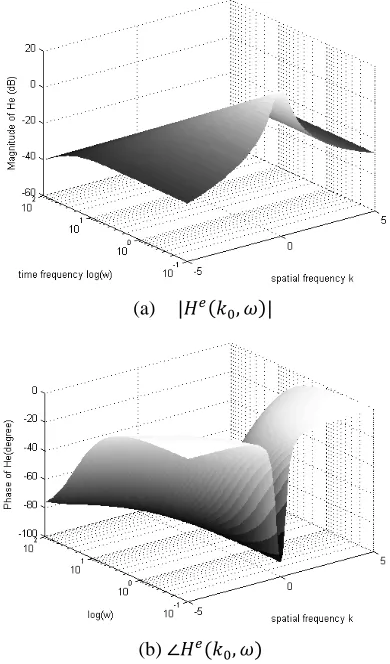
(44) Suppose the input to (44) is , then the probing method gives the frequency response function as

(45) The magnitude and phase of (45) with are shown in Fig. 1, where Fig. 1 (a) shows that system (44) works as a low-pass filter with respect to both space and time frequencies. The frequency domain response depends on both space and time frequencies. These interact with each other. For example, for a certain spatial frequency , is a first order linear system and the corner frequency of the first order system increases with the increase of .

(a)

(b)

The frequency response is related to the following problem

(46) Suppose the input to (46) is , the output and the associated temporal and spatial derivatives are then

(47) Substituting (47) and into equation (46) yields

(48) The frequency response function can be obtained as the solution to the initial value problem (48)

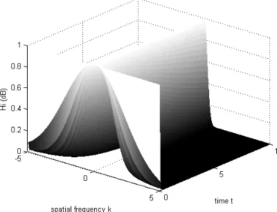
(49) By taking a inverse Fourier Transform, the impulse response function can be obtained as

(50) Fig. 2 shows that the response excited by initial conditions declines with elapsing time. An initial condition with a high frequency sharply drops to zero while a low frequency initial condition declines with a relatively lower speed.

Fig. 2 with of Example A

B. Nonlinear Spatio-temporal Systems – Fisher’s Equation

Consider the following Fisher’s equation in dimensionless form (Debnath 2005)

(51) where D is the diffusion coefficient. In this example, only the first and second order generalized frequency responses will be calculated. An initial condition

yields

(52) Equating the coefficients of on both sides yields

(53) so that the first order generalised frequency response is

(54) In order to calculate , suppose the input is , the corresponding output is

(55) The probing method gives

(56) Substituting (54) into (56) yields

(57) The general solution of (57) can be represented as

(59) The generalised frequency response with respect to

initial conditions is given by

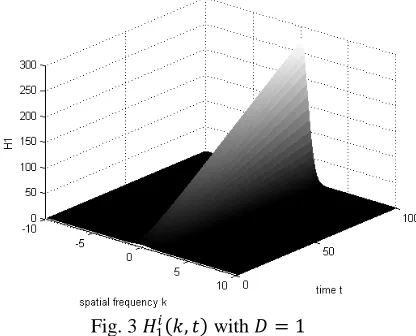
(60) Figs. 3 and 4 show the spatio-temporal generalised frequency response functions and , respectively.

Fig. 3 with

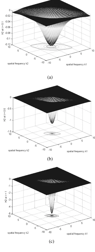
Figs. 3 and 4 show that the magnitude for both

and increase with elapsing time for low frequency initial conditions while they decrease with elapsing time for high frequency initial conditions. When , the stability condition for is

and the stability condition for is

(61) which have been shown in Fig. 5.

V. CONCLUSIONS

The concept of classical transfer functions and frequency responses have been extended to both linear and nonlinear spatio-temporal systems which are defined over an unbounded spatial domian. It has been shown, through a theoretical analysis and numerical examples, that the proposed generalised transfer functions and frequency response functions are consistent with the classical definitions. A new method for identifying and computing the generalised frequency response functions for spatio-temporal systems has also been presented. The definitions and methodology

introduced in this paper provide a solid basis and powerful tools for further investigations of the spectral analysis and properties of spatio-temporal systems.

ACKNOWLEDGEMENTS

The authors gratefully acknowledge support from the UK Engineering and Physical Sciences Research Council (EPSRC) and the European Research Council (ERC).

REFERENCES

Bedrosian, E. and Rice, S. O. (1971), The output properties of Volterra systems (nonlinear systems with memory) driven by harmonic and Gaussian inputs, Proceedings IEEE, Vol. 59, pp. 1688-1707.

Billings, S. A. and Wei, H. L. (2007), Characterising linear spatio-temporal dynamical systems in the frequency domain, Research Report 944, The University of Sheffield.

Billings, S. A. and Peyton-Jones, J. C. (1990), Mapping nonlinear integro-differential equations into the frequency domain, Int. J. Cont, Vol.52, pp. 863-879.

Billings, S. A. and Tsang, K. M. (1989a), Spectral analysis for non-linear systems, Part I: parametric non-linear spectral analysis, Mechanical Systems and Signal Processing, Vol.3, No.4, pp. 319-339. Billings, S. A. and Tsang, K. M. (1989b), Spectral analysis for non-linear systems, Part II: Interpretation of non-linear frequency response functions, Mechanical Systems and Signal Processing, Vol.3, No.4, pp. 341-359.

Curtain, R. F., and Morris, K. (2009), Transfer functions of distributed parameter systems: A tutorial, Automatica, Vol, 45, pp. 1101-1116.

Curtain, R. F., and Zwart, H. J. (1995), An Introduction to Infinite-Dimensional Linear Systems theory, New York: Springer-Verlag.

Debnath, L. (2005), Nonlinear partial differential equations for scientists and engineers (2nd ed.), Boston: Birkhauser.

Garcia-Sanz, M., Huarte, A., and Asenjo, A. (2007), A quantitative robust control approach for distributed parameter systems, Int. J. Robust Nonlinear Control, Vol. 17, pp. 135–153.

Goodman, J. (2005), Introduction to Fourier Optics (3rd ed), USA: Roberts & Co Publishers.

Guo, L. Z., Guo, Y. Z., Billings, S. A., Coca, D., and Lang, Z. Q. (2010), Spatio-temporal generalised frequency response functions over bounded spatial domain, Research Report, The University of Sheffield.

Guo, Y. Z., Billings, S. A., Coca, D., Peng, Z. K., and Lang, Z. Q. (2009), Characterising spatio-temporal dynamical systems in the frequency domain, Research Report 1000, The University of Sheffield. Marmarelis, P. Z. and Marmarelis, V. Z. (1978), Analysis of Physiological Systems – the White Noise Approach, New York: Plenum Press.

Peyton-Jones, J. C. and Billings, S. A. (1989), A recursive algorithm for computing the frequency response of a class of nonlinear difference equation model, Int. J. Cont, Vol.50, pp. 1925-1940.

Qiao, B. and Ruda, H. E. (2004), Green functions for nonlinear operators and application to quantum computing, Physica A: Statistical Mechanics and its Applications, Vol. 334, No. 3-4, pp. 459-476.

Rabenstein, R. and Trautmann, L. (2002), Multidimensional transfer function models, IEEE Trans. Circu. & Syst.- Fundamental Theory and Application, Vol. 49, No.6, pp. 852-861.

Schetzen, M. (1980), The Volterra and Wiener Theories of Nonlinear systems, Chichester: John Wiley.

Schwartz, C. (1997), Nonlinear operators and their propagators, Journal of Mathematical Physics, Vol. 38, No. 1, pp. 484-500.

Trim, D. W. (1990), Applied Partial Differential Equations, Boston: PWS-Kent Publishing Company.

Zadeh, L. (1950), Frequency analysis of variable network, Proceedings of The I.R.E., Vol. 38, pp. 291-299.

(a)

(b)

(c)

(d)

Fig. 4 with (a) , (b) , (c) , (d)