Pre-main-sequence variability across the radiative-convective gap

Pre-main-sequence variability across the radiative–convective gap

Eric S. Saunders,

Tim Naylor,

Nathan Mayne

and S. P. Littlefair

2_{School of Physics, University of Exeter, Stocker Road, Exeter EX4 4QL} 3_{Department of Physics and Astronomy, University of Sheffield, Sheffield S3 7RH}

Accepted 2009 April 17. Received 2009 April 17; in original form 2009 February 23

A B S T R A C T

We useI-band imaging to perform a variability survey of the 13-Myr-old cluster h Per. We find a significant fraction of the cluster members to be variable. Most importantly, we find that variable members lie almost entirely on the convective side of the gap in the cluster sequence between fully convective stars and those which have a radiative core. This result is consistent with a scenario in which the magnetic field changes topology when the star changes from being fully convective to one containing a radiative core. When the star is convective, the magnetic field appears dominated by large-scale structures, resulting in global-size spots that drive the observed variability. For those stars with radiative cores, we observe a marked absence of variability due to spots, which suggests a switch to a magnetic field dominated by smaller-scale structures, resulting in many smaller spots and thus less apparent variability. This implies that wide field variability surveys may only be sensitive to fully convective stars. On the one hand, this reduces the chances of picking out young groups (since the convective stars are the lower mass and therefore fainter objects), but conversely the absolute magnitude of the head of the convective sequence provides a straightforward measure of age for those groups which are discovered.

Key words: stars: fundamental parameters – Hertzsprung–Russell (HR) diagram – stars: magnetic fields – stars: pre-main-sequence – stars: spots – stars: variables: other.

1 I N T R O D U C T I O N

Despite the widespread use of the photometric variability of young stars to study their rotational evolution (see Herbst et al. 2007, for a review), its underlying causes remain poorly understood. The variability itself appears to be due to a combination of (in the order of importance) coolspots, hotspots, obscuration and pul-sation (Krzesi´nski, Pigulski & Kołaczkowski 1999; Carpenter, Hillenbrand & Skrutskie 2001; Grankin et al. 2007, 2008). We know these stars have kG magnetic fields (e.g. Johns-Krull 2007), and all these sources of variability are probably related to those fields. The coolspots are large starspots; the hotspots are probably due to accre-tion funnelled on to a small region of the star by the magnetic field and the obscuration is again due to magnetically confined accretion structures. A largely unexploited route to elucidate the underlying physics of the resulting optical variability is to study its character-istics as a function of fundamental stellar parameters, such as mag-netic field, age and accretion rate. Variability caused by pulsation will be of the order of millimagnitudes, and so is difficult to observe. Additionally, variability caused by obscuration due to circumstellar or disc material is expected to be negligible for h Per, as at≈13 Myr

_{E-mail: [email protected] (ESS); [email protected] (NM)}

(Slesnick, Hillenbrand & Massey 2002; Mayne et al. 2007) most of the associated discs and circumstellar material would probably have dissipated. However, variability caused by large coolspots or accretion hotspots generates significant magnitude changes over periods of hours to days, and therefore is relatively simple to detect. Here, we study the degree of variability, caused by hot-and coolspots, as a function of stellar mass in the young clus-ter, h Per. The mass range covered by our data includes stars ei-ther side of the transition from low-mass fully convective to stars with radiative cores [the point in the colour–magnitude diagram (CMD) Mayne et al. (2007) call the radiative–convective (RC) gap].

The target of our investigation, h Per, and its companion,χPer, are young, bright open clusters that have been the subject of detailed observations for 70 years (e.g. Oosterhoff 1937; Crawford, Glaspey & Perry 1970; Tapia et al. 1984; Waelkens et al. 1990). More recently, attention has been focused on their mass functions and mass segregation (Slesnick et al. 2002; Bragg & Kenyon 2005). We adopt an age of 13 Myr (Slesnick et al. 2002; Mayne et al. 2007), although the precise value is not crucial for our work.

our findings and their implications. Finally, Section 5 presents a short conclusion.

2 M E T H O D

The observations were taken using a Sloanifilter with the 2.5-m Isaac Newton Telescope (INT) on La Palma, using the Wide Field Camera with four EEV CCDs. The run spanned 16 nights, from 2004 September 22 to October 7. h Per was observed on 12 of these nights, for around 2.5 h per night. Exposures of 5, 30 and 300 seconds were obtained. There were 213 good frames taken with 300 s exposure, and 110 good frames for each of 5 and 30 s exposure.

2.1 Data reduction

The data were reduced, and then photometry extracted using the optimal extraction algorithm of Naylor (1998) and Naylor et al. (2002), with the modifications introduced by Littlefair et al. (2005). The images were bias subtracted using a single master bias frame, corrected for flat-field effects using twilight sky flat-field images, and defringed. For each exposure time, we chose a single frame, and then searched the combination of the three to create a master catalogue. The objects were then matched to a Two-Micron All Sky Survey (2MASS) catalogue of our field to produce an astrometric solution, with a mean rms discrepancy in position of 0.1 arcsec.

For each image, positional and rotational offsets were determined with respect to the master catalogue. Using the list of candidate objects, we performed optimal photometry on individual frames to produce fluxes for each star in each image.

Next, a ‘profile correction’, the logical analogue of an aperture correction in standard aperture photometry, was applied to correct the flux measured for our objects to a somewhat larger aperture (although the crowded nature of the field limits this). A number of bright, unsaturated stars in each CCD provided the profile correction for that CCD, which is a polynomial function of position. Although our photometry is relative, and not tied to any particular system, this correction is still important because the spatial variation of the point spread function (PSF) is a function of the seeing (Littlefair et al. 2005).

From this point, we separated the photometry by exposure time into three data sets. For each data set, a relative transparency correc-tion was applied to all the resulting photometric measurements, to normalize any differences between frames arising from variations in airmass or transparency. This was achieved by selecting a subset of relatively bright, unvarying stars and using their average magni-tude to define a reference brightness for each frame. This was done in the same way as described in Littlefair et al. (2005).

The photometry for a star in each data set is only relative photom-etry with respect to the other stars in that data set. To produce the final catalogue, the data sets were renormalized using the magni-tude ranges for which they overlapped. We then applied an arbitrary zero-point to our instrumental magnitude so that our observations would be in a natural magnitude system approximately comparable with Sloani. We denote magnitudes in this system by the symbol iI. Of course, many stars have magnitudes from more than one data set, but for consistency it is important we create each light curve from a single data set, and that we use the same data set for stars of similar mean magnitudes. Thus, the 5 s data set was used for all stars brighter than aniIof 15.2. Light curves for stars with 15.2< iI<17.5 were taken from the 30 s data set, while for stars fainter than iI = 17.5 light curves were taken from the 300 s data set.

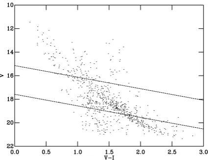
Figure 1. CMD of the variable population, after combining the 5, 30 and 300 s data sets (724 objects). The dashed lines indicate the limiting magni-tudes (discussed in Section 2.1) used to combine the data sets. The fact that the sequence appears unbroken across the boundaries means that the selec-tion criteria will not be a funcselec-tion of magnitude and therefore sensitivity.

These characteristic or limiting magnitudes are shown plotted over the data as dashed lines in Fig. 1.

2.2 Variable star selection

The identification of variable stars involved a set of distinct se-lection criteria. First, the data set was stripped of stars flagged as problematic during the data reduction process. Data-quality checks made during this process included identifying duplicate de-tections of the same star, stars containing bad or saturated pixels, pixels with counts in the non-linear response range of the detector and pixels with negative counts. Additionally, stars possessing a PSF that was not point-like were flagged for non-stellarity. A num-ber of spurious variables at the corner of CCD 3 were removed due to high vignetting, using a simple coordinate cut. We then selected only those light curves with a mean signal-to-noise ratio per frame of more than 10.

Having dealt with the most obviously problematic objects, we next considered the light curves themselves. The ideal data set would have the same number of data points for each light curve, allowing us to use a simpleχ2 _{cut to identify variable stars. Of}

course, many light curves have missing data points for a variety of reasons, which means that we should choose a different value ofχ2_{for each light curve if we require identical probabilities that}

the light curves show variability. In practice, for a large number of degrees of freedom, the distribution of reducedχ2_{is such that the}

probability associated with a givenχ2

νis almost independent ofν.

This means if we pick only those light curves with a large number of data points, we can apply a simpleχ2

νcut-off. Such an approach

has the advantage that even if our model of the uncertainties is not perfect (in particular there may be correlated noise in the data), the cut-off will be consistent. So, we required a minimum of 60 good data points from the 5 and 30 s data sets (from a possible 110), and 120 good data points from the 300 s data set (from a possible 213). To make our analysis more robust against single spurious data points we discarded the data point with the highest individualχ2

with respect to the weighted mean, before re-calculating the mean, and henceχ2

ν.

Following Littlefair et al. (2005), we chose a threshold ofχ2

ν>

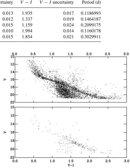
Table 1. Periods for the five strongest periodic variable candidates in our sample.

ID RA Dec. V Vuncertainty V −I V −Iuncertainty Period (d)

1.01 1293 02 20 44.582 +56 54 56.35 18.948 0.013 1.935 0.017 0.1186993 1.02 1325 02 17 46.554 +57 04 18.08 18.312 0.012 1.337 0.019 0.1464187 1.02 2157 02 18 01.071 +56 53 56.73 18.770 0.015 1.159 0.024 0.2099175 1.04 0251 02 20 21.400 +57 03 22.03 18.685 0.010 1.994 0.014 0.1160178 1.04 1906 02 20 28.387 +57 03 03.66 19.325 0.015 1.854 0.021 0.3029911

The correctχ2

ν limit for the 30 s data set was then determined by

considering stars falling within the overlap region between the two data sets. Varying the value ofχ2

ν applied to the 30 s data set, we

found that a threshold ofχ2

ν>3 recovered a number of variable stars

in this region that was comparable to the number of stars detected in the 300 s data set. Similarly, by considering variables identified in both the 5 and 30 s data set, it was found that aχ2

ν>3 threshold

applied to the 5 s data set recovered all variables toiI≈15.2. This process yielded 724 significantly varying objects from the initial list of 19 860 objects with good-quality light curves.

2.3 Periodic Variability

One might hope to reduce the contamination still further by consid-ering only those stars which have periodic modulation. Although our data set is not well suited for identifying periods, caused by magnetically formed spots on the stellar surface, in the likely range for pre-main-sequence stars (a few hours to≈20 d), we did carry out an exploratory period search, summarized in Table 1. The period search was performed following the method described in Littlefair et al. (2005). Final analysis of the shortlist of variables was made by visual inspection of individual light curves. Here, we show our best candidates for periodic variability, along with a note of their position in the CMD. The number of periodic variables is clearly too small for our analysis, and so we instead use the catalogue of variable stars to create CMDs.

2.4 Colour–magnitude diagrams

To create CMDs for the variable stars, we cross matched our cata-logue of variable stars against the h andχPer catalogue of Mayne et al. (2007). This gave theV versusV −I CMD with 724 ob-jects shown in Fig. 1. To enhance the contrast between the cluster and the contaminating stars (see Section 3), we also created CMDs from both our variable star catalogue and the Mayne et al. (2007) catalogues for a 10 arcmin radius region centred on the cluster (α= 02 18 58.76,δ= +57 08 16.5 J2000). With this spatial cut, these catalogues have 230 and 3840 objects, respectively, plotted in Fig. 2.

3 R E S U LT S

Fig. 1 shows a clear pre-main-sequence population running diago-nally from approximately 14th to 20th magnitude inV. However, background contamination is also evident. The contamination is more obvious in the upper panel of Fig. 2 where it covers a large, wedge-shaped area that cuts laterally across the sequence. The ma-jority of this wedge is likely to be dwarfs, but the additional ‘finger’ atV − I ≈ 1.6 is probably due to background giants. As de-scribed in Section 2.4, to reduce this contamination we selected only those variable stars which are within 10 arcmin of the cluster core.

Figure 2. CMD of photometry towards h Per showing a clear sequence of probable members, including variables, taken from Mayne et al. (2007) (upper panel), and variables only (lower panel) after a 10 arcsec radial cut centred on h Per. The upper panel has 3840 objects; the lower, 230. The number of variables drops atV−I <1.5.

Fig. 2 (lower panel) shows the variables remaining after this pro-cess. We can clearly see that the density of stars falls dramatically as we progress up the sequence. This is quite different from the distribution of cluster members (Fig. 2, top panel), which shows a narrow sequence up to around 15th magnitude.

3.1 Histogram analysis

Although it is clear from visual inspection of the sequence that the density of variable stars in the CMD falls dramatically at brighter magnitudes, additional analysis is required to investigate this be-haviour in a robust way. Because we wish to examine the distribu-tion of variables along the cluster sequence, we construct histograms according to the following scheme. A straight line was fitted to the central portion of the sequence, running from 1.0 to 2.0 inV −I. Two lines perpendicular to this sequence line inV /V −I space (i.e. appearing perpendicular to the sequence when both axes are plotted with units of equal size) were then taken, a bright cut cross-ing the sequence at 1.0 inV −I and a faint cut crossing at 1.66 (see Fig. 3). We selected the stars within 0.4 mag of these lines and then pulled them back on to the cut centre lines and binned them in V −I. Identical cuts were used for the h Per catalogue of Mayne et al. (2007). These cuts produce the histograms of Fig. 4.

Figure 3. Placement of cuts along the line of the sequence of h Per variables. Stars falling within either of the cuts are represented as crosses. Identical cuts were used to analyse the general cluster membership.

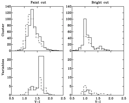
Figure 4. Histograms of the lower cut (left-hand images) and upper cut (right hand images), binned along the line of the cut. The upper pan-els show non-variables, while the lower panpan-els present only stars exhibit-ing significant variability. The solid line indicates objects fallexhibit-ing within a 10 arcmin circle of the h Per centre. The dashed line is a count of the stars falling outside that cut, normalized to the same area as the cut. The dashed lines thus measure the background contamination present in the field.

trace the sequence at 1.6–1.7 in colour. The sequence can also be seen in the histogram for the general cluster (Fig. 4, top-left panel), as a shoulder of excess sources over the background, although in this case the contamination dominates between 1.0 and 1.5 in V −I. The fact that these stars are mostly contaminants is evi-denced by the large number of background objects present in the sky around the cluster at these colours (dashed line, normalized to the same area as the selected area of the cluster). Note that the blue end of the contamination appears to be shifted bluewards, relative to the foreground cluster. This could be due to differential reddening (Capilla & Fabregat 2002).

In the brighter magnitude cut (Fig. 4, top-right image), the cluster is significantly less contaminated, with more than half of the stars additional to the background. However, looking at the variables (Fig. 4, bottom-right image) presents a different picture. There are relatively few variables present either in the background or in the se-quence. In fact, the number of variables is consistent with a scenario in which there are no variables present in the sequence.

The position of the two cuts was chosen to bracket the RC gap (as defined and identified in h Per by Mayne et al. 2007), where the stars move from the fully convective regime to the development of a radiative core. Therefore, these data and the chosen cuts allow us to analyse changes in the fraction of variables on either side of this gap. Integrating under the histograms of Fig. 4 allows us to construct the background-subtracted numbers of variable and non-variable stars, and calculate the fraction of stars which are variable, both above and below the gap. We find that below the gap 37.9 per cent of stars are variables, above it−1.7 per cent. The latter is negative as the total (background plus cluster) number of variables is so small that its associated noise means that background subtraction can push it below zero. This means that we actually see less variables in this region of the CMD than the mean number we would expect to be contributed by background objects. To test the significance of this difference, we formed the null hypothesis that the fraction of variables above the gap is the same as that below the gap, i.e. 37.9 per cent. We then used the Poisson distribution to simulate observations of the stars above the gap, using parent populations identical to our observations, save that for cluster stars above the gap we changed the fraction of variables to 37.9 per cent. In one million simulations, we never obtained an observed fraction of variable stars less than or equal to−1.7 per cent. This allows us to reject the null hypothesis that the ratio of members to variable stars is constant on either side of the RC gap with great confidence, and conclude that the variable stars do indeed die out as one moves above the gap.

4 D I S C U S S I O N

4.1 A break at the RC gap?

Stolte et al. (2004) and Mayne et al. (2007) show that in CMDs there is a discontinuity in the stellar sequence between pre-main-sequence and main-pre-main-sequence stars, which Mayne et al. (2007) term the RC gap. Below this gap, theory predicts that the stars are fully convective, whilst above it they possess radiative cores. This gap closes with age, becoming very small for objects as old as h Per. For stars above the gap, one model postulates that the magnetic field is generated at the tachocline between the radiative core and the convective envelope. In this model, it is believed that shearing processes in this layer generate a magnetic field, although the full picture may well be more complicated (e.g. Choudhuri, Schussler & Dikpati 1995). For fully convective stars, the source of the field is more controversial. On the one hand, a turbulent velocity field might create a small-scale magnetic field (Durney, De Young & Roxburgh 1993). Alternatively, Chabrier & K¨uker (2006) showed that a stratified rotating medium might create a large-scale magnetic field (theα2_dynamo).

a modulation, if any, below our threshold of detection. Thus, our observations are consistent with the idea that whilst fully convec-tive stars have large-scale structure in their magnetic fields, once the stars develop a radiative core the spots become more evenly distributed over the surface. Whilst it can still be argued whether the magnetic field is due to convective turnover (Chabrier & K¨uker 2006), turbulence (Durney et al. 1993) or fossil field (Tayler 1987), what this study makes clear is that the fully convective structure is a crucial ingredient for the maintenance of the large-scale magnetic fields of T Tauri stars.

4.2 Comparison with older field stars

Further support for a change in magnetic field topology at the RC gap can be found from recent studies using Zeeman Doppler imag-ing of older field dwarfs, where the same physical mechanisms are apparent, i.e. fully convective lower mass stars and higher mass objects with radiative cores. These studies have found sig-nificant evidence for a sharp reduction in magnetic flux, contained within large-scale structures, as one moves across the boundary (in mass) between fully convective stars and those with radiative cores. Donati et al. (2008) and Morin et al. (2008) compare observations of the StokesVline profiles for old field dwarfs about the boundary of radiative core presence (atM_∗≈0.35 M using the evolution-ary models of Chabrier & Baraffe 1997), to simulated profiles from estimated magnetic maps of the stellar surface. The StokesV mea-surements are sensitive to large-scale magnetic fields, rather than small-scale structures, which have opposite polarities that cancel in the StokesVprofile. Donati et al. (2008) and Morin et al. (2008) find a clear difference in magnetic fields, with large-scale poloidal, axisymmetric fields dominant for fully convective stars, and only toriodal and non-axisymmetric poloidal fields apparent over large scales for stars with radiative cores. Measurements of X-ray ac-tivity and the total magnetic field from the Zeeman broadening show little change at the radiative core boundary (see discussion in Donati et al. 2008), implying only a structural change in the mag-netic field, possibly due to the theorized change in dynamo mecha-nism. Additionally, for fully convective stars these large-scale struc-tures were observed to be stable over≈1 yr with stability over only a few months for the magnetic structures of stars with radiative cores.

Further work using StokesIobservations, which is sensitive to the total magnetic field, in Reiners & Basri (2009) has similarly ob-served a sharp change in apparent field structure over the transition from fully convective stars to those with a radiative core. Reiners & Basri (2009) find, by comparing StokesV andI components, that across this boundary (i.e. the RC gap) the percentage of total flux stored in large-scale structures drops from 15 to 6 per cent, with the presence of a radiative core. The mean total flux does not show a comparable jump. Interestingly, Reiners & Basri (2009) show that 85 per cent of the flux is not detected in StokesV and therefore is present in small-scale structures. Additionally, they note that the weak-field assumption and least-squares deconvolution method ap-plied in Donati et al. (2008) and Morin et al. (2008) could lead to large-scale fields of several kG being missed. This may mean that the change in magnetic field structure with the transition from full convective to radiative core could simply be due to an increase in field strength of the large-scale structures over the detectable thresh-old. This scenario is currently untestable, but is unlikely given our observations. Our data indicate a change in photometric variability and therefore magnetic field structure with the presence of a ra-diative core. If this is the same mechanism as is postulated for the

older field stars, and is indeed the result of a transition in stellar structure, then the change in variability observed across the RC gap arises from a fundamental change in magnetic field topology, itself a consequence of a change in the dynamo mechanism.

4.3 Implications for future variability surveys

Variability will be an important technique for identifying young stellar associations in large area variability surveys such as the Large Synoptic Survey Telescope (e.g. Brice˜no et al. 2007). Fig. 2 shows what such a survey should discover. Only the sequence below the RC gap is visible in the variability data, which reduces the chances of finding the cluster. However, the variability data clearly show where the RC gap begins. Since the position of the RC gap fades with age, measuring this position provides a new technique for measuring the age of a group, which will be useful well beyond 20 Myr. This contrasts sharply with the results of Mayne et al. (2007), who concluded that the distance across the RC gap would become unusable as an age indicator for groups older than h Per, since the gap closes to be extremely small. Thus, it appears that although the RC gap in CMDs alone may no longer provide ages for these older systems, a CMD of the variable stars could do so.

5 C O N C L U S I O N

In conclusion, we have measured, and proved the statistical signif-icance of, a reduction in the number of variable stars, compared to non-variables, as one moves from below to above the RC gap in h Per. We have discussed the connection between this reduc-tion in variability across the gap and underlying changes in the stellar magnetic fields. We suggest that this distinct reduction in variability could be due to a change in the magnetic field topology caused by a change in stellar structure, from fully convective stars to those with radiative cores. This idea implies that the fully con-vective stars retain large-scale stable surface magnetic fields, which lead to long-lived coolspots on the stellar surface, and therefore long-term variability. In contrast, for stars with a radiative core the magnetic field becomes dominated by smaller-scale structures pro-ducing more transient and less significant variability. It is clear that variability surveys will therefore be biased towards the detection of the fainter, fully convective, stars within clusters. However, the bright edge of the RC gap, where the variability dies out, could be used as an age indicator.

AC K N OW L E D G M E N T S

ESS and NM were funded through PPARC studentships. SPL is supported by an RCUK fellowship and PPARC grant PPA/G/S/2003/00058. The INT is operated on the island of La Palma by the Isaac Newton Group in the Spanish Observatorio del Roque de los Muchachos of the Institute de Astrofisica de Canarias. We would also like to thank the referee for an in depth review and helpful comments.

N OT E A D D E D I N P R O O F

the internal structure of the stars. They identify this break at a

V−I∼1.3–1.7, which agrees convincingly with our position of the RC gap (V−I∼1.5).

R E F E R E N C E S

Bragg A. E., Kenyon S. J., 2005, AJ, 130, 134

Brice˜no C., Preibisch T., Sherry W. H., Mamajek E. A., Mathieu R. D., Walter F. M., Zinnecker H., 2007, in Reipurth B., Jewitt D., Keil K., eds, Protostars and Planets V. Univ. Arizona Press, Tucson, p. 345 Capilla G., Fabregat J., 2002, A&A, 394, 479

Carpenter J. M., Hillenbrand L. A., Skrutskie M. F., 2001, AJ, 121, 3160 Chabrier G., Baraffe I., 1997, A&A, 327, 1039

Chabrier G., K¨uker M., 2006, A&A, 446, 1027

Choudhuri A. R., Schussler M., Dikpati M., 1995, A&A, 303, L29 Crawford D. L., Glaspey J. W., Perry C. L., 1970, AJ, 75, 822

Currie T., Evans N. R., Spitzbart B. D., Irwin J., Wolk S. J., Hernandez J., Kenyon S. J., Pasachoff J. M., 2009, AJ, 137, 3210

Donati J.-F. et al., 2008, MNRAS, 390, 545

Durney B. R., De Young D. S., Roxburgh I. W., 1993, Sol. Phys., 145, 207 Grankin K. N., Melnikov S. Y., Bouvier J., Herbst W., Shevchenko V. S.,

2007, A&A, 461, 183

Grankin K. N., Bouvier J., Herbst W., Melnikov S. Y., 2008, A&A, 479, 827

Herbst W., Eisl¨offel J., Mundt R., Scholz A., 2007, in Reipurth B., Jewitt D., Keil K., eds, Protostars and Planets V. Univ. Arizona Press, Tucson, p. 297

Johns-Krull C. M., 2007, ApJ, 664, 975

Krzesi´nski J., Pigulski A., Kołaczkowski Z., 1999, A&A, 345, 505 Littlefair S., Naylor T., Burningham B., Jeffries R. D., 2005, MNRAS, 358,

341

Mayne N. J., Naylor T., Littlefair S. P., Saunders E. S., Jeffries R. D., 2007, MNRAS, 375, 1220

Morin J. et al., 2008, MNRAS, 390, 567 Naylor T., 1998, MNRAS, 296, 339

Naylor T., Totten E. J., Jeffries R. D., Pozzo M., Devey C. R., Thompson S. A., 2002, MNRAS, 335, 291

Oosterhoff P. T., 1937, Ann. Sterre. Leiden, 17, 1 Reiners A., Basri G., 2009, A&A, 496, 787

Slesnick C. L., Hillenbrand L. A., Massey P., 2002, ApJ, 576, 880 Stolte A., Brandner W., Brandl B., Zinnecker H., Grebel E. K., 2004, AJ,

128, 765

Tapia M., Roth M., Costero R., Navarro S., 1984, Rev. Mex. Astron. Astrofis., 9, 65

Tayler R. J., 1987, MNRAS, 227, 553 Waelkens C. et al., 1990, A&AS, 83, 11