Replanning for situated robots

Replanning for Situated Robots

Michael Cashmore

and

Andrew Coles

King’s College London

Bence Cserna

University of New Hampshire

Erez Karpas

Technion — Israel Institute of Technology

Daniele Magazzeni

King’s College London

Wheeler Ruml

University of New Hampshire

Abstract

Planning enables intelligent agents, such as robots, to act so as to achieve their long term goals. To make the planning pro-cess tractable, a relatively low fidelity model of the world is often used, which sometimes leads to the need to replan. The typical view of replanning is that the robot is given the cur-rent state, the goal, and possibly some data from the previous planning process. However, for robots (or teams of robots) that exist in continuous physical space, act concurrently, have deadlines, or must otherwise consider durative actions, things are not so simple. In this paper, we address the problem of replanning for situated robots. Relying on previous work on situated temporal planning, we frame the replanning problem as a situated temporal planning problem, where currently ex-ecuting actions are handled via Timed Initial Literals (TILs), under the assumption that actions cannot be interrupted. We then relax this assumption, and address situated replanning with interruptible actions. We bridge the gap between the low-level model of the robot and the high-level model used for planning by the novel notion of abail out action gen-erator, which relies on the low-level model to generate high-level actions that describe possible ways to interrupt currently executing actions. Because actions can be interrupted at dif-ferent times during their execution, we also propose a novel algorithm to handle temporal planning with time-dependent durations.

Introduction

The connection between planning and execution is a seem-ingly simple one: a robot will typically first plan, that is, come up with a course of action that achieves its goal, and then execute that plan. However, planning is usually done using a relatively low fidelity model, in order to make the planning process tractable. This can lead to the not-infrequent need to replan. Other possible causes for replan-ning include newly sensed information, failure to execute some action (while other actions might still continue exe-cuting), or the goal changing.

The typical view of replanning is that the robot is given its current state, its goal, and possibly some data from the pre-vious planning process (e.g., the prepre-vious plan or the gener-ated search nodes). If the robot actually existed in a world that obeyed the assumptions of classical planning, then this

Copyright c2019, Association for the Advancement of Artificial Intelligence (www.aaai.org). All rights reserved.

would indeed be correct. However, for robots (or teams of robots) that exist in continuous physical space, act concur-rently, have deadlines, or must otherwise consider durative actions, things become more complex. Consider, for exam-ple, a durative encoding of a MOVE(A,B) action, which ap-pears in many planning domains. This action is meant to model a robot moving from waypointAto waypointB. It is usually modeled as deleting at(A) in the beginning, and adding at(B)at the end. Now consider the state of the world, and specifically the location of the robot, if replanning is triggered while the MOVE action is executing. Since at(A) was already deleted, but at(B) was not yet added, the robot is currently nowhere. This discrepancy is caused by the fact that the robot is actually located at some real set of coor-dinates, but planning uses an abstraction of the real world consisting of waypoints. This mismatch will cause a naive replanning process to fail.

In this paper, we propose a general solution to this lem. Our overall approach is to frame the replanning prob-lem as planning with adynamicinitial state. This dynamic initial state is modeled by a temporal planning problem, which captures the effects and conditions of currently ex-ecuting actions using timed initial literals (TILs) (Cresswell and Coddington 2003; Edelkamp and Hoffmann 2004).

Our first treatment of this problem assumes that actions are non-interruptible and that, once an action has started, it will either continue executing until it succeeds or it will fail and trigger replanning. We show how previous work on sit-uated temporal planning (Cashmore et al. 2018) can be used to handle the dynamic initial state described above, and thus is also useful for replanning while actions are currently exe-cuting.

However, forcing an agent to complete an action it has started can be highly suboptimal. For example, consider a rover driving to waypointAto sample a rock there. Suppose halfway through the drive, the agent realizes that the drill is stuck, making drilling impossible, and thus invalidating the plan and triggering replanning. Forcing the rover to finish the drive toAis pointless, as it no longer has any actions to perform atA. Even worse, this wastes time and consumes battery energy, which could have been used to achieve other goals. Thus, we will also address the case where actions can be interrupted.

a higher fidelity model of the world, which makes model-ing difficult and plannmodel-ing intractable. Thus, we assume only carefully limited use of such a model, in the form of a black-box ‘bail out action’ generator that, based on a more de-tailed model of the agent’s state, can propose various ways to bail out of a currently executing action. For example, a bail out action generator for move actions might generate paths from the real position of the robot to several nearby waypoints. Importantly, bailout actions arelocal, in that they only describe ways to bail out of a currently executing ac-tion. Thus, instead of planning with one high-fidelity model of the world, which could be difficult to come up with, we can plan with one low-fidelity model combined with several models for bail out actions, which do not necessarily have to be consistent with each other or account forallaspects of the problem.

Recall that time still passes while we are replanning, and the robot’s real position when replanning is triggered may be different from its real position when the new plan will start executing, and thus the duration of the bail out action will be different depending on when it begins execution. However, as we explain later, thesetime-dependent durationsobey a certain monotonicity property, namely that the ending time of the bailout action is monotonic in its start time — that is, the earlier the bailout action is triggered, the earlier it completes. We present a novel algorithm for checking the consistency of a Simple Temporal Network (STN) (Dechter, Meiri, and Pearl 1991) with such monotonic time-dependent durations, which we have integrated with the OPTIC planner (Benton, Coles, and Coles 2012).

We evaluate our approach on a real robotic testbed — a Turtlebot robot in an office delivery task, as well as in the Robocup Logistics League (RCLL) simulation (Niemueller, Lakemeyer, and Ferrein 2015). Our results show that our re-planning approach outperforms a baseline which can only plan from a static state, either when there are deadlines in the problem, or when there are multiple agents which our approach can better exploit.

Related Work

Action failures, goal changes, and other online execution is-sues have long been facts of life in the planning commu-nity. One way to cope is to produce plans in a representa-tion with inherent flexibility, such as representing exact exe-cution times as a temporal constraint network (Ghallab and Laruelle 1994), or to return partial policies, such as contin-gent plans (Pell et al. 1997; Myers 1999). When the only uncertainty is about action durations, planning can be com-bined with scheduling under uncertainty to come up with ro-bust plans (Cimatti et al. 2018). However, trying to account for uncertain outcomes often impedes scalability.

Another way to handle change is to replan. For example, when plans for their printing system are invalidated by bro-ken machine modules, Ruml et al. (2011) attempt to rescue in-flight sheets by replanning the remainder of their trajec-tories. This requires estimating the time required by replan-ning, so that an appropriate state can be chosen at which the new plan will replace a suffix of the original plan.

Planning online is also explored in Domain Predictive Control (L¨ohr et al. 2013; 2014), which combines planning with Model Predictive Control to generate control input se-quences for hybrid dynamical systems. Perhaps the most closely related work to ours is the IxTeTeXEC executive (Lemai and Ingrand 2004), which interleaves planning and execution, and takes into consideration the fact that execu-tion will start only after planning finishes.

Fox et al. (2006) contrast replanning with plan repair, and argue that the latter can promote plan stability, the similarity of a new plan to the original. In applications involving multi-agent coordination or multi-level planning, stability can pro-vide benefits. Cushing and Kambhampati (2005) propro-vide a counter-argument, arguing that plan repair can be subsumed by replanning where, among other changes, the objective of the new planning problem might penalize deviating from the commitments of the previous plan. This allows an agent to properly balance the costs and benefits of using actions sim-ilar to those in the original plan. All of this previous work assumes that failures conveniently happen at action bound-aries and that the world stops while the agent replans.

Cashmore et al. (2018) consider planning problems in which actions depend on externally timed events, such as taking a bus, and the time taken during planning can be long enough to affect the choices of the planner. For example, if planning is anticipated to take a long time, plans involving taking the next bus may not be found soon enough to be ex-ecutable. They develop a strategy in which externally timed events are modeling using TILs and estimates of remaining planning time are used to prune infeasible heuristic search nodes in the planner.

Preliminaries

We consider propositional temporal planning problems with Timed Initial Literals (TIL) (Cresswell and Coddington 2003; Edelkamp and Hoffmann 2004). Such a planning problem Π is specified by a tuple Π = hF, A, I, T, Gi, where:

• F is a set of Boolean propositions that describe the state of the world.

• Ais a set of durative actions. Each actiona ∈ Ais de-scribed by:

– Minimum duration durmin(a) and maximum dura-tion durmax(a), both in R0+ with durmin(a) ≤ durmax(a),

– Start condition cond`(a), invariant condition

cond↔(a), and end condition conda(a), all of which are subsets ofF, and

– Start effect eff_`(a) and end effect eff_a(a), both of which specify which propositions in F become true (add effects), and which become false (delete effects).

• I⊆Fis the initial state, specifying exactly which propo-sitions are true at time 0.

• G⊆F specifies the goal, that is, which propositions we want to be true at the end of plan execution.

A solution to a temporal planning problem is a schedule

σ, which is a sequence of triplesha, ta, dai, wherea ∈ A is an action,ta ∈ R0+is the time when actionais started, andda∈[durmin(a),durmax(a)]is the duration chosen for

a. A schedule can be seen as a set of instantaneous happen-ings(Fox and Long 2003) that occur when an action starts, when an action ends, and when a timed initial literal is trig-gered. Specifically, for each tripleha, t, diin the schedule, we have actionastarting at timet(requiringcond`(a)to hold a small amount of timebefore timet, and applying the effectseff<sub>`</sub>(a)right att), and ending at timet+d (re-quiringconda(a)to holdbefore t+d, and applying the effectseff_a(a)at timet+d). For a TILlwe have the effect specified bylit(l)triggered at timetime(l). Finally, in or-der for a schedule to be valid, we also require the invariant conditioncond↔(a)to hold over the open interval between

tandt+d, and that the goalGholds at the state which holds after all happenings have occurred.

Interruptible and Non-Interruptible Actions

As previously mentioned, actions might be interruptible or non-interruptible. A high-level propositional model does not necessarily capture this difference. Consider two actions, both of which move an object from waypointAto waypoint

B:

Ballistic Launch:The action is implemented by launching an object using a catapult.

Driving:The action is implemented by driving.

Both of these actions can be modeled withpre_`=at(A),

eff_` = ¬at(A), eff_a = at(B), with a controllable du-ration in the range[dmin, dmax]. However, for the ballistic launch action, the duration is chosen when the action is ex-ecuted (by setting the appropriate trajectory), and can not be changed during execution — that is, the action is non-interruptible.

On the other hand, for the driving action, the duration is, in fact, a different way of representing the average veloc-ity. If this action is interrupted, the duration can be adjusted, or the agent can even choose to drive to any other location. However, all of these options are not modeled in the standard propositional representation of this action.

In the next section, we explain how we address situated replanning with only non-interruptible actions, by relying on previous work on situated temporal planning (Cashmore et al. 2018). Then, we describe one way of modeling inter-ruptible actions, and how we can replan with interinter-ruptible actions for situated agents, that is, online.

Replanning with Non-interruptible Actions

We now describe our approach for replanning during exe-cution with non-interruptible actions. For example, consider the well known match cellar domain, in which a fuse must be fixed while a match is burning. The LIGHT-MATCH ac-tion serves as an envelope for the FIX-FUSE acac-tion; that is, FIX-FUSE must be executed within the time interval when

F0=F∪ {ea| ha, ta, dai ∈CA}

A0={a0|a∈A},where:

durmin(a0) =durmin(a)

durmax(a0) =durmax(a)

cond`(a0) =cond`(a)∪

{eb| hb, tb, dbi ∈CA,del`(a)∩cond↔(b)6=∅}

cond↔(a0) =cond↔(a)

conda(a0) =conda(a)∪

{eb| hb, tb, dbi ∈CA,dela(a)∩cond↔(b)6=∅}

eff`(a 0

) =eff`(a)

effa(a 0

) =effa(a)

I0=I

T0={htime(l)−t,lit(l)i |l∈T,time(l)≥t}∪ {hta+da−t, fi | ha, ta, dai ∈CA, f∈eff`(a)}∪

{hta+da−t, eai | ha, ta, dai ∈CA

G0=G

Figure 1: Replanning Task Definition

LIGHT-MATCH is executing. Now assume that FIX-FUSE failed for some reason, but we have already lit our only re-maining match. Thus, we must come up with a plan and be able to execute it within the remaining time until LIGHT-MATCH has finished.

One decision we make here is that, when replanning has been triggered, we never start executing a new action from the original scheduleπ— we only finish executing the cur-rently executing actions. This is because we do not yet know whether future actions in the (stale) plan might lead to a dead end, in which case we will never be able to solve the prob-lem. Thus, we choose to possibly err on the side of inaction, and deal only with the currently executing actions. We are also assuming here that, if action failure triggered replan-ning, the failed actions had either no effect on the state or that the effects of the failure are fully observed and modeled at the start of replanning.

In general, letΠ =hF, A, I, T, Gibe the planning prob-lem, and assume we are in the process of executing a sched-uleπwhen replanning is triggered at timet, when the cur-rent state of the system is s. As previously mentioned, it would be incorrect to simply replan from states, because (a) there might be some actions which have already started but have not yet ended, and their invariant conditions and end effects must be taken into consideration, and (b) the TILs in

Π0, described fully in Figure 1, is very similar toΠ, except that it contains a facteafor each currently executing action, which indicates that the action has finished. The ea facts work together with TILs (as explained below) and slightly modified action definitions to enforce the invariant condi-tions of currently executing accondi-tions, as we now explain.

The TILs inΠ0 capture three different things. First, we adjust the timing of the TILs from the original planning task, to reflect that the current time ist, so past TILs are removed, and the time for future TILs is adjusted by decreasing it byt. Second, we use TILs to encode the end effects of currently executing actions, so that if action a will finish in dtime units, its effects are encoded as TILs which will occur at time

d. Finally, we use TILs to signal that an action has ended (by settingea to true), and therefore its invariant condition no longer has to hold. This, in turn, enables all snap actions (start or end of a durative action) which delete the invariant condition ofa— which is implemented by addingea as a condition for all snap actions whose effects delete some fact incond↔(a).

We can now use previous work on situated temporal plan-ning (Cashmore et al. 2018) to solve the above planplan-ning task. Since this technique accounts for time passing while plan-ning is going on, the solution returned by the planner will be executable when the planner terminates — even if the cur-rently executing actions have not finished yet.

To continue the above example, suppose the duration of LIGHT-MATCH is 10 seconds, and FIX-FUSE failed 2 sec-onds after LIGHT-MATCH started. We encode this using a TIL, stating that the end effect of LIGHT-MATCH (i.e., the light going out) will occur 8 seconds from when replanning started. Essentially, this imposes a deadline of 8 seconds on goal achievement time (GAT) — that is, planning time + plan makespan, which the situated temporal planner can ac-count for.

Replanning with Interruptible Actions

We now turn our attention to the problem of replanning with interruptible actions. As previously mentioned, we must first overcome the issue of modeling what are the possible ways to bail out of a currently executing action. We assume we have access to a bail out action generator, which takes as in-put an action (that is assumed to be currently executing — we still do notstart executing actions from the stale plan before a new plan is found), and returns as output a list of possiblebail out actions. The bail out action generator can be thought of as extending the successor generator with al-ternative endings of the currently executing action. This bail out generator can be implemented as a black box, and will run every time replanning is triggered. Thus, the bail out ac-tion generator can have access to lower level state variables than the high-level propositional model used for planning does.

Although the details of bail out actions are domain-specific, there are common properties that we discuss. Es-sentially, the most important property of a bail out action is that, after the bail out action has ended, the high-level propo-sitional planning model isconsistent. In other words, the bail

out action needs to correctly specify the high-level proposi-tional state of the worldafterthe bail out action has finished, which ensures that after applying a bail out action, we can keep planning using the more abstract high-level proposi-tional model.

For example, consider the previous example of a rover driving from waypointAto waypointB to sample a rock, when the drill breaks at some point during the drive. The bail out action generator can utilize a path planner, which has access to the rover’s real position (and possibly even to the underlying dynamical model which accounts for mass, acceleration, obstacles, turning radius, . . . ). These bail out actions restore the state of the world to a consistent one, where after the bail out action finishes the rover has a loca-tion, instead of not being located anywhereduringthe drive. When modeling bail out actions for high-level proposi-tional planning, a good rule of thumb is that a bailout action forashould have something to do with the state variablesa

affects. In light of the abovementioned discussion on restor-ing consistency, this means that when we model a bail out action fora, we should start by looking at the effects ofa, and identify facts which are made inconsistent by the start effects ofa, whose consistency is restored by the end effects ofa. Our bail out action should fix those, but of course, the low-level details of the domain could dictate other precondi-tions and effects for the bail out acprecondi-tions.

An additional complication occurs when considering the fact that multiple actions could be executing currently, and bailing out of them might not be independent. For example, consider a rover that is driving fromAtoB, and taking pic-tures of the route from A toB — which can be modeled using two concurrently executing actions: drive(A, B)and photo(A, B). In this case, bailing out of drive(A, B) also requires bailing out of photo(A, B). If we have such co-dependent actions, our bail out generator could take as input sets of currently executing actions, and generate options to bail out of all of the input actions. As implied by the above discussion, such co-dependency will typically occur only for actions which have some shared fact in their preconditions or effects.

Durations of Bail Out Actions

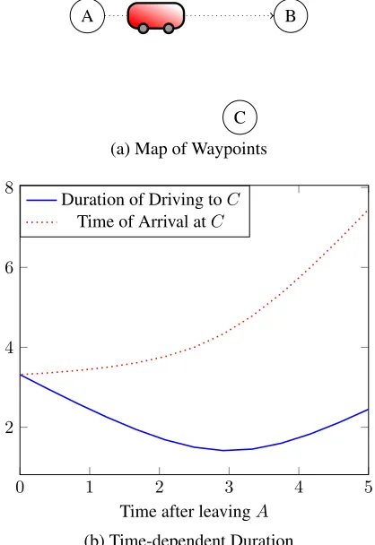
We now turn our attention to the durations of the bail out ac-tions. Continuing with our rover example, consider the map illustrated in Figure 2a, where the rover is driving from A

toB, and replanning is triggered when it is in the position drawn in the figure, about one third of the way fromAtoB. One possible bail out action is to drive to C. The duration of this bail out action depends on the position of the rover, which in turn depends on the time the bail out action starts. Thus, in order to plan in such a scenario, we must extend our planner to handle time-dependent durations. Furthermore, this time-dependent duration could be non-monotonic. In our example, the duration decreases until the rover reaches the point on the line fromAtoB where it is closest toC, and starts increasing after passing that point, as illustrated in Figure 2b (the solid blue line).

A B

C

(a) Map of Waypoints

0 1 2 3 4 5

2 4 6 8

Time after leavingA

Duration of Driving toC

Time of Arrival atC

(b) Time-dependent Duration

Figure 2: Illustration of Rover Example

can start, denotedestimated latest start(π). This estimate relied on both the current planπ as well as the Temporal Relaxed Planning Graph (TRPG) (Coles et al. 2010) from the state reached byπ. Unfortunately, with non-monotonic time-dependent durations, it is not enough to look at a single number to describe the latest time a plan can start.

Note, however, that theending timeof the bailout action does increase monotonically with the time the bail out ac-tion started, as shown in the dotted red line in Figure 2b. We claim this is always the case, under some reasonable as-sumptions, which we discuss next.

Optimal Bailout Actions and Monotonicity

Recall that our bailout action generator has access to a higher fidelity model of the world, although it plans for a shorter horizon. If this planner returns optimal plans, then the ending time of the bailout action should always increase monotonically with when the bail out action started.

In our rover example, where we ignore obstacles, the shortest path toCis a straight line. The rover travels on the straight line fromAtoBfor some distanced, and then bails out and drives in a straight line towardsC. Clearly, the to-tal distancethe rover travels on the way toC, and thus the duration, increases withd, although not necessarily linearly. To formalize this intuition, assume that each high-level actionacorresponds to a planπa=hl1, l2, . . . , lmiin some higher-fidelity (low-level) model of the world, whereli are

low-level actions. We also assume the bailout action gener-ator uses an optimal planner for this low-level model, min-imizing the total duration of the plan. Finally, assume the agent bails out ofaafter executinghl1, l2, . . . , lni, and de-note the low-level state of the world at this time byxn.

Now consider what happens if the agent bails out earlier, aftern0 < nlow-level actions. Note that we are assuming the same bailout target, that is, the same goal in the low-level model in both cases. We will denote this bailout goal bybg. It is easy to see that the optimal plan fromxn0tob_gcan not be more expensive than any plan which continues the execution ofauntillnand then bails out tobg, that is, a plan fromxn0 tobgwhich is constrained to start withhln0₊₁, . . . , l_ni. Thus, if our bailout action generator relies on an optimal planner, we automatically get monotonicity in the ending time of the bailout action.

However, it is also easy to show examples where this property does not hold. If our bailout action generator calls a sampling-based motion planner, e.g., RRT (Lavalle, Kuffner, and Jr. 2000), then we can not guarantee that it returns an op-timal path. Nevertheless, if we ever get such low level plans that bailing out at timet1 finishes later than bailing out at timet2, butt1 < t2, we can always improve upon the bail out action at timet1, by continuing execution of the origi-nal action until timet2, and bailing out then. In other words, because it is always possible to bail out later, we can ob-tain monotonicity in the ending time of bail out actions via simple post processing of the durations of the bail out ac-tions, which chooses the best time to bail out after some time point, instead of exactly at that time point.

We have seen the monotonic nature of the ending time of bail out actions. We now explain how we exploit this prop-erty in checking the temporal consistency of partial plans with time-dependent durations, which is integrated into our temporal planner.

Temporal Planning with Time-Dependent

Durations

In prior temporal planners (Coles et al. 2010; 2009), the tem-poral constraints on a plan under construction have been rep-resented as a Simple Temporal Problem (Dechter, Meiri, and Pearl 1991) – a collection of constraints, eachlb≤tj−ti≤

ub, withub,lb∈ <+₀, recording the constraints on the tem-poral separation of the plan stepsti andtj. State progres-sion updates an STP stored in each state, according to the actions applied. Then, by solving the STP, one can deter-mine whether the temporal constraints are consistent; and if so, obtain the minimum and maximum time at which each step can be scheduled. In the nominal case, in temporal plan-ning, only the minimum times are used when reporting the time-stamps of a solution plan.

Algorithm 1:STP with Time-Dependent Durations Data:STP constraintsT and the corresponding plan of

snap-actionsP

Result:ts, the timestamps of the plan steps inP; or⊥

if the STP is inconsistent

1 Ttd ← ∅; 2 do

3 ts←solve to find minimum timestamps of the STP

(T∪Ttd);

4 ifts=⊥then return⊥; 5 converged ← >;

6 Ttd ← ∅;

7 foreachstart–end snap action pairha`, aai ∈P, with step indexesiandjrespectivelydo 8 dur ←duration ofaif started at timets[i]; 9 min dur←minimum time-dependent duration

ofaat any time at-or-afterts[i];

10 max dur ←maximum time-dependent

duration ofaat any time at-or-afterts[i];

11 addts[i] +dur ≤tjtoTtd;

12 addmin dur ≤tj−ti≤max durtoTtd; 13 if¬(dur≤ts[j]−ts[i]≤dur)then 14 converged ← ⊥;

15 end

16 while¬converged; 17 returnts

be applied is known.

To address this issue, we take a two-fronted approach. First, during search, when applying an actionawith a time-dependent duration that starts at stepiand finishes at stepj, the STP is constrained soacan have any duration between its global minimum and global maximum – across any of the times for which its duration is defined. This admissibly relaxes the time-dependency into a duration interval.

Second, when checking that the temporal constraints in a given state are consistent – formerly a case of simply check-ing the consistency of the STP – an iterative refinement pro-cess is used, presented in Algorithm 1, which exploits the monotonicity requirement on the durations of bailout ac-tions.

The algorithm takes as input the STPT from the state, as well as the plan P that reached it, and builds a collec-tion of addicollec-tional STP constraintsTtd to capture the

time-dependent durations. On the first iteration, these are empty, hence at line 3 the STP solved is that from the state – if this is inconsistent, the algorithm terminates immediately.

Otherwise, the algorithm then inspects the times given to actions, to see what time-dependent durations are relevant – assuming they started at-or-after the times ints, withts[i]

denoting the time of stepi. For each start–end action pair in the plan, with step indexesiandj, we look up three values:

• What the duration of the action would be if it started ex-actly attimets[i]– the durationdur

• What the minimum possible duration of the action would be, assuming it has to comeat or aftertimets[i] – the durationmin dur

• What the maximum possible duration of the action would be, assuming it has to comeat or after timets[i] – the durationmin dur

These values are used in two ways. First, ‘feasibility cuts‘ are added toTtd, as follows:

• ifdur is indeed the duration the action should have, the earliest time stepjcould occur ists[i] +dur(line 11).

• in any case, starting the action at or after timets[i]bounds its duration betweenmin durandmax dur (line 12).

Second, the value ofduris used to determine whether the current solution to the STP is consistent with respect to the time-dependent durations. If this is not the case (i.e.ts[j]− ts[i] 6= dur – line 13) the converged flag is set to false – indicating that the algorithm must continue to iterate.

The correctness of this algorithm exploits the monotonic-ity requirement of bailout actions; i.e. that delaying the start of a bailout actionmayreduce its duration, butmay notlead to a net reduction in the time at which the action can end. If this were not the case, then search would be needed at line 11: we would lose the ability to determine an admissi-ble lower-bound on the end time of an action based on its start time and the duration it would have at that time, as a better end-time may be attainable by delaying the start.

The algorithm is guaranteed to converge due to the be-havior of the feasibility cuts. For the cuts delaying the ends of actions, the cuts on one iteration dominate those in the previous iteration: the ends of actions are iteratively de-layed, but never made earlier. Delaying the ends of ac-tions may in turn delay the starts of other acac-tions; and in-creasing the start time of an action only ever reduces the range [min dur,max dur] until there is only one option left – i.e. the duration is no longer time-dependent. Then, as dur = min dur = max dur, the cut added toTtd on

line 12 guarantees that on subsequent iterations, the duration constraint will always be satisfied. At the limit, all actions are assigned their latest possible time-dependent duration, so none of the duration constraint checks at line 13 will lead toconvergedbeing set to>; so the loop terminates.

Empirical Evaluation

In order to empirically evaluate our approach to replanning, we evaluated it on problems from the Robocup Logistics League (RCLL) Simulation (Niemueller, Lakemeyer, and Ferrein 2015; Niemueller et al. 2016), and on a real robotic system. We compare our approach to a baseline which can only replan from a static state. Thus, we formulate a plan-ning problem whose initial state is the state that will hold when all currently executing actions finish. However, we use a situated temporal planner (Cashmore et al. 2018) which can plan while the currently executing actions finish. We force this planner to only start executing after all currently executing actions finish by adding a new facte(which stands for execute), which is added by a TIL when all currently ex-ecuting actions finish, and is a start condition of all actions.

# 1 Robot 2 Robots 3 Robots

R B R B R B

5 9.635 9.635 0.05 0.35

15 45.158 45.654 100.961 54.258 77.46 18 15.55 15.551 34.131 38.1 1.041 1.041 28 63.998 60.527 144.902 49.325 49.325 32 62.267 56.488 60.331 16.79 18.102 34 129.301 83.464 57.541 73.139 124.393 35 82.102 82.429 63.517 47.817 31.401 31.401 39 55.526 179.377 162.422 52 60.78 41.672

55 18.299 18.3 132.501 136.862 56 52.746 42.526 51.004 57.145

57 43.959 43.948 69.007 5.942 5.942 64 41.899 46.577 16.698 26.688 100.72 165.269 68 59.974 59.256 123.063 108.989 74.078 71 60.992 50.979 9.564 9.564 73 22.76 22.76 44.677 85.833 84.632

78 52.162 222.93 112.392

80 0.803 0.803 46.24 46.24 71.078 72.462 81 66.478 98.285 54.74 27.62 27.62 86 134.195 97.714 95.733 84.247 155.941 89 12.038 12.038 134.84 48.361 146.077 91 133.342 127.479 55.047 76.08 52.872 69.099 99 66.826 65.996

SOLVED 21 23 15 17 13 17

Avg. GAT 56.34 51.53 60.99 60.07 44.13 50.11

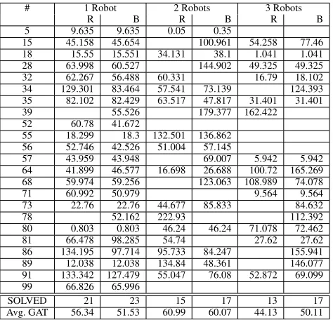
Table 1: Goal Achievement Time on RCLL Instances for Baseline (B) and Our Replanning Approach (R) for In-stances with no Deadline

start planning after all currently executing actions have fin-ished. However, this is clearly inferior to the baseline we used, and thus we omit it from the experiment.

We now describe each of these experiments in detail.

RCLL

The Robocup Logistics League Challenge presents a plan-ning problem where 3 robots must fulfill orders that arrive dynamically by feeding workpieces to 6 different machines. Each machine can perform one type of processing step, and fulfilling an order requires performing a series of process-ing steps on different machines. Each order can also have a deadline — we ran one experiment on a version with dead-lines and another on a version without deaddead-lines.

In order to trigger replanning, we first generate a plan to solve the original problem. Then we randomly choose some point in the plan (using a uniform distribution), choose one of the machines at random (also uniformly), and trigger re-planning by simulating a failure of the chosen machine. Un-like in the original challenge, we assume that when the ma-chine fails, it will be fixed at some known time in the future, which is also chosen randomly between 10% to 30% of the makespan of the original plan. As we do not modify robot behaviors here, we did not implement a bail out action gen-erator, and we assume actions are non-interruptible.

For this experiment, we started with 100 random RCLL instances generated for a previous paper (Schaepers et al. 2018). For each of these problems we have 3 versions: with 1, 2, or 3 robots. We only used the 23 instances which were solved within our time limit of 200 seconds for all 3 versions of the problem. We triggered replanning for all 3 versions of each of these 23 instances, and compare our proposed approach here with the baseline.

# 1 Robot 2 Robots 3 Robots

R B R B R B

5 1.791 1.791 0.05 0.28 10.456 10.456 15 8.702 8.702 57.258 80.907 149.369 18 55.39 54.412 57.189 97.039 66.225 28 44.316 45.669 149.862 51.997 83.426 32 34.751 34.751 46.474 78.681 34 36.054 36.054 64.219 69.711 59.348 57.063 35 114.534 116.784 48.013 68.772 39 67.44 45.394 67.384 56.848 52 43.267 47.299 108.064 56.795 59.125 55 66.745 56.732

56 18.947 18.948 86.399 97.877 36.816 71.843 57 46.221 26.152 26.152 59.144 59.144 64 92.747 111.351 91.723 65.061

68 49.312 51.866 32.655 32.655 71 106.72 99.832 72.467 73 52.142 72.753 72.285 125.065 78 8.756 8.756 55.687 70.239 146.216 80 59.327 58.357 79.032 76.492

81 132.003 61.396 51.084 58.399 70.166 86 2.707 2.707 17.911 17.912 89 42.057 46.896 4.144 4.144 33.411 33.411 91 114.602 123.41 53.322 60.394 68.341 99 50.697 50.697 84.643 86.475 106.005 SOLVED 21 23 14 17 14 17 Avg. GAT 54.8 51.51 53.77 59.92 44.68 55.42

Table 2: Goal Achievement Time on RCLL Instances for Baseline (B) and Our Replanning Approach (R) for In-stances with Deadline

The experiments were run on a virtual machine running on powerful laptop (Intel Core-i7 8750H CPU). 6 planners were run in parallel using the parallel tool (Tange 2011), each with a time limit of 200 seconds and no memory limit (the VM had 16 GB of virtual memory).

The results for problems without a deadline are described in Table 1 and those for the version with a deadline in Table 2. Both of these tables show the goal achievement time (GAT) from when replanning was triggered, as well as the total number of problems solved and the average GAT (which is taken over the instances solved by both approaches for each number of robots).

The picture in both tables is similar and as expected: for 1 robot, there is no benefit in our replanning approach. This is because each robot can only execute a single action at any given moment, and thus there is no benefit to using our more sophisticated replanning approach. The overhead of our ap-proach, which creates a larger planning problem, is also evi-dent here with the smaller number of problems solved. How-ever, as the number of robots increases, our approach ben-efits, as it has more opportunities to start executing actions with one or two robots while the others complete their cur-rently executing actions.

Real Robotic System: Office Delivery

immedi-Problem 1 2 3 4 5 6 7 8

Bailout 777.568 824.573 841.183 620.600 339.760 514.008 795.625 901.881

Baseline - - -

-Problem 9 10 11 12 13 14

Bailout 1587.022 1177.209 1177.207 1656.577 1061.984 1098.133

Baseline - 1169.432 - - 1136.626

-Table 3: GAT for problems in the Office Delivery scenario. Times in seconds. ”-” denotes that the problem was made unsolvable due to deadlines passing while waiting for actions to complete.

Figure 3: The Turtlebot 2 platform used in the second exper-iment to perform delivery tasks.

ately recharge).

The domain for the robot includes navigation actions be-tween waypoints, actions for requesting and waiting for hu-man assistance, and assisted pick and place actions. In addi-tion the domain includes acaddi-tions for docking to recharge, un-docking, and localizing the robot, which must be performed after each recharge and before navigation can begin. Replan-ning typically occurs while the robot is navigating between two locations and the charge level drops below the replan-ning threshold.

As this is a real robotic system, we also implemented a bail out action generator for the navigation actions the robot performs. The bailout action generator for moving fromA

toB along some pathpgenerates a bailout action of going to some other waypointC. This is implemented as follows:

1. Sample points along the current pathpat intervals of 4 meters.

2. From each sampled pointx, a collision-free path is com-puted by the default global planner of the ROS navigation package. This path planner applies Dijkstra’s algorithm to the global 2D costmap.

3. The duration of the bailout action is time-dependent: we compute the time of arrivalti to each sampled pointxi along the original path p. While the time from when move(A, B) started is betweenti−1 andti, the duration of bailing out to C is the sum ofti and the duration of following the computed path from xi toC. We remark that even though the path planner is not optimal, we did not have to perform the post processing described above to enforce monotonicity of the ending times.

Using the bail out action generator allows the robot to de-cide, when replanning is triggered, to cancel the currently

executing action and instead execute the bailout action. To perform this experiment, we integrated the approach we describe here, as well as the new planner which sup-ports time-dependent durations, with ROSPlan (Cashmore et al. 2015). As ROSPlan has already been integrated with the Turtlebot 2, no extra effort was required there. The only programming required for integrating the research described here with ROSPlan was extending the system such that the bailout action generator described above is called every time replanning is triggered (by ROSPlan, this time). To do this the ROSPlan Problem Interface was extended to call the bailout generator. This node generates the PDDL problem instance to be solved by the planner. The planning problem that is generated is solved by calling the new planner. To integrate the new planner, no changes needed to be made.

The goal achievement time is shown in Table 3. The ex-periment consists of 14 problems, each containing 4-5 deliv-ery goals. The delivdeliv-ery destinations and deadlines were ran-domized, with deadlines between 3 and 25 minutes. We used two sets of problems. In the first set (problems 1 – 8, in the upper half of Table 3), there was only one possible bail out destination: the dock. In the second set of problems (prob-lems 9 – 14, in the lower half of Table 3), there were multiple possible bail out destinations: the dock and all other charg-ing stations throughout the office. For each problem, replan-ning was triggered manually immediately after dispatching the first navigation action. As these results show, using the baseline approach of waiting for the currently executing ac-tion to complete renders the problem unsolvable due to the deadlines on the delivery tasks in almost all cases.

Summary and Future Work

In this paper, we have addressed replanning for situated agents. The contributions of this paper are threefold: First, we framed the problem of situated replanning with execut-ing actions as a temporal plannexecut-ing problem with a dynamic initial state, utilizing TILs. Second, we introduced the notion of bail out action generators, which bridge the gap between the high-level model used for planning and the low-level re-alistic model, and allow us to interrupt currently executing actions. These bail out actions lead to actions with time-dependent durations, and thus our third contribution deals with temporal reasoning with time-dependent durations.

not interrupt currently executing actions, and each agent is limited to performing only one action at a time, then our approach is only beneficial if there are multiple agents, and thus one agent can start executing actions even before all the other agents have finished their actions. As the experiment on real robots shows, our approach is especially useful with long action durations.

Finally, we remark that although this paper addresses re-planning, we have not made use of the previous plan. In future work, we will explore ways of exploiting the previ-ous plan, by integrating some plan reuse or repair techniques (Fox et al. 2006) into our framework.

References

Benton, J.; Coles, A. J.; and Coles, A. 2012. Temporal planning with preferences and time-dependent continuous costs. InProceedings of the 22nd International Conference on Automated Planning and Scheduling (ICAPS).

Cashmore, M.; Fox, M.; Long, D.; Magazzeni, D.; Ridder, B.; Carrera, A.; Palomeras, N.; Hurt´os, N.; and Carreras, M. 2015. Rosplan: Planning in the robot operating system. In Proceedings of the 25th International Conference on Auto-mated Planning and Scheduling (ICAPS), 333–341. Cashmore, M.; Coles, A.; Cserna, B.; Karpas, E.; Maga-zzeni, D.; and Ruml, W. 2018. Temporal planning while the clock ticks. In de Weerdt, M.; Koenig, S.; R¨oger, G.; and Spaan, M. T. J., eds., Proceedings of the Twenty-Eighth International Conference on Automated Planning and Scheduling, ICAPS 2018, Delft, The Netherlands, June 24-29, 2018., 39–46. AAAI Press.

Cimatti, A.; Do, M.; Micheli, A.; Roveri, M.; and Smith, D. E. 2018. Strong temporal planning with uncontrollable durations. Artif. Intell.256:1–34.

Coles, A.; Fox, M.; Halsey, K.; Long, D.; and Smith, A. 2009. Managing concurrency in temporal planning us-ing planner-scheduler interaction. Artificial Intelligence 173(1):1–44.

Coles, A. J.; Coles, A.; Fox, M.; and Long, D. 2010. Forward-chaining partial-order planning. InProceedings of the 20th International Conference on Automated Planning and Scheduling (ICAPS), 42–49.

Cresswell, S., and Coddington, A. 2003. Planning with timed literals and deadlines. InProceedings of 22nd Work-shop of the UK Planning and Scheduling Special Interest Group, 23–35.

Cushing, W., and Kambhampati, S. 2005. Replanning: a new perspective. InProceedings of ICAPS-05.

Dechter, R.; Meiri, I.; and Pearl, J. 1991. Temporal con-straint networks. Artificial Intelligence49(1-3):61–95. Edelkamp, S., and Hoffmann, J. 2004. PDDL2.2: The lan-guage for the classical part of the 4th international planning competition. Technical Report 195, University of Freiburg.

Fox, M., and Long, D. 2003. PDDL2.1: an extension to PDDL for expressing temporal planning domains. Journal of Artificial Intelligence Research (JAIR)20:61–124.

Fox, M.; Gerevini, A.; Long, D.; and Serina, I. 2006. Plan stability: Replanning versus plan repair. InProceedings of ICAPS-06, 212–221.

Ghallab, M., and Laruelle, H. 1994. Representation and con-trol in IxTeT, a temporal planner. InProceedings of AIPS-94, 61–67.

Lavalle, S. M.; Kuffner, J. J.; and Jr. 2000. Rapidly-exploring random trees: Progress and prospects. In Algo-rithmic and Computational Robotics: New Directions, 293– 308.

Lemai, S., and Ingrand, F. 2004. Interleaving temporal plan-ning and execution in robotics domains. InAAAI, 617–622. L¨ohr, J.; Eyerich, P.; Winkler, S.; and Nebel, B. 2013. Do-main predictive control under uncertain numerical state in-formation. InProceedings of the Twenty-Third International Conference on Automated Planning and Scheduling, ICAPS 2013, Rome, Italy, June 10-14, 2013.

L¨ohr, J.; Wehrle, M.; Fox, M.; and Nebel, B. 2014. Symbolic domain predictive control. InProceedings of the Twenty-Eighth AAAI Conference on Artificial Intelligence, July 27 -31, 2014, Qu´ebec City, Qu´ebec, Canada., 2315–2321. Myers, K. 1999. Cpef: A continuous planning and execution framework.AI MAgazine.

Niemueller, T.; Karpas, E.; Vaquero, T.; and Timmons, E. 2016. Planning Competition for Logistics Robots in Simu-lation. InICAPS Workshop on Planning and Robotics (Plan-Rob).

Niemueller, T.; Lakemeyer, G.; and Ferrein, A. 2015. The RoboCup Logistics League as a Benchmark for Planning in Robotics. InWS on Planning and Robotics (PlanRob) at Int. Conf. on Aut. Planning and Scheduling (ICAPS).

Pell, B.; Gat, E.; Keesing, R.; Muscettola, N.; and Smith, B. 1997. Robust periodic planning and execution for au-tonomous spacecraft. InProceedings of IJCAI-97.

Ruml, W.; Do, M. B.; Zhou, R.; and Fromherz, M. P. J. 2011. On-line planning and scheduling: An application to control-ling modular printers. Journal of Artificial Intelligence Re-search40:415–468.

Schaepers, B.; Niemueller, T.; Lakemeyer, G.; Gebser, M.; and Schaub, T. 2018. ASP-based time-bounded planning for logistics robots. In Proceedings of the 28h Interna-tional Conference on Automated Planning and Scheduling (ICAPS).