Video Saliency Detection Using Object Proposals

Video Saliency Detection Using Object Proposals

Fang Guo, Wenguan Wang, Jianbing Shen , Senior Member, IEEE,

Ling Shao , Senior Member, IEEE, Jian Yang, Dacheng Tao , Fellow, IEEE,

and Yuan Yan Tang, Fellow, IEEE

Abstract—In this paper, we introduce a novel approach to

identify salient object regions in videos via object proposals. The core idea is to solve the saliency detection problem by ranking and selecting the salient proposals based on object-level saliency cues. Object proposals offer a more complete and high-level representation, which naturally caters to the needs of salient object detection. As well as introducing this novel solution for video salient object detection, we reorganize various discrimina-tive saliency cues and traditional saliency assumptions on object proposals. With object candidates, a proposal ranking and voting scheme, based on various object-level saliency cues, is designed to screen out nonsalient parts, select salient object regions, and to infer an initial saliency estimate. Then a saliency optimization process that considers temporal consistency and appearance differences between salient and nonsalient regions is used to refine the initial saliency estimates. Our experiments on public datasets (SegTrackV2, Freiburg–Berkeley Motion Segmentation Dataset, and Densely Annotated Video Segmentation) validate the effectiveness, and the proposed method produces significant improvements over state-of-the-art algorithms.

Index Terms—Object proposals, object-level saliency cues,

salient region detection, video saliency.

I. INTRODUCTION

S

Manuscript received February 6, 2017; revised June 2, 2017 and August 20, 2017; accepted October 2, 2017. This work was supported in part by the National Key Research and Development Program of China under Grant 2017YFC0107900, in part by the National Science Foundation Program of China under Grant 61672099, Grant 81430039, Grant 81627803, Grant 61527827, and Grant 61272359, in part by the Australian Research Council Projects under Grant FL-170100117, Grant DP-140102164, and Grant LP-150100671, in part by the Fok Ying-Tong Education Foundation for Young Teachers, and in part by the Specialized Fund for Joint Building Program of Beijing Municipal Education Commission. This paper was recommended by Associate Editor H. Lu. (Corresponding author: Jianbing Shen.)

F. Guo, W. Wang, and J. Shen are with the Beijing Key Laboratory of Intelligent Information Technology, School of Computer Science, Beijing Institute of Technology, Beijing 100081, China (e-mail: [email protected]).

L. Shao is with the School of Computing Sciences, University of East Anglia, Norwich NR4 7TJ, U.K. (e-mail: [email protected]).

J. Yang is with the Beijing Engineering Research Center of Mixed Reality and Advanced Display, School of Optoelectronics, Beijing Institute of Technology, Beijing 100081, China (e-mail: [email protected]).

D. Tao is with the UBTECH Sydney Artificial Intelligence Centre and the School of Information Technologies, Faculty of Engineering and Information Technologies, University of Sydney, Darlington, NSW 2008, Australia (e-mail: [email protected]).

Y. Y. Tang is with the Faculty of Science and Technology, University of Macau, Macau 999078, China (e-mail: [email protected]).

Color versions of one or more of the figures in this paper are available online at http://ieeexplore.ieee.org.

Digital Object Identifier 10.1109/TCYB.2017.2761361

vision applications, intensive research has been carried out for salient object detection to identify the most important or noticeable object regions [1], [2], [61]. Those methods try to highlight the whole salient object regions, which diverge from the early saliency prediction algorithms that focus on locating human eye fixations [3]. Generally, salient object detection models generate large and smoothly connected salient areas. In this paper, we proposed a novel video salient object detec-tion algorithm toward locating primary salient objects in dynamic scenes. It produces a gray-scale saliency map for each video frame, where brighter pixels indicate higher saliency values.

Traditional salient object detection models for videos are mainly based on bottom-up mechanisms. These models uti-lize various low-level features (e.g., color and motion) and heuristics (e.g., feature contrast between region/pixels and the surrounding area) [2], [5], [8]. Although these bottom-up saliency models achieve inspiring results, they still have several limitations. In particular, they do not yield consistent saliency values for a complete salient object or for the whole background, especially when an object has multiple compo-nents or the background is cluttered. This phenomenon arises because bottom-up techniques take pixels or superpixels as basic units to infer saliency. From the perspective of human perception, it would be more natural to work on the com-plete object level. Pixel or superpixel level mechanisms lack of object-level features, thus they cannot completely meet the goal of locating salient object regions. However, this problem has not yet to be addressed in existing algorithms.

To bridge the gap between low-level saliency cues and object-level salient object detection, we explore salient object detection based on object-level cues namely object proposal. For an input image, object proposal methods generate a set of category-independent object candidates which are likely to include the object of interest. Thus, those object candidates are able to cover entire objects in the image with excellent accuracy [34]. With candidates for an object in hand, vari-ous traditional saliency cues can be extracted and reorganized to improve the saliency estimates. Recently, Zhang et al. [6] grouped superpixels to form the potential local salient regions and construct a local saliency measure with the reconstruc-tion errors. However, the key idea of the suggested model is leveraging object-level information for detecting salient object. Based on this, the proposed model reorganizes various saliency cues and heuristics. Besides, our model detects saliency in dynamic scenes, while Zhang et al. [6] concentrated more on detecting salient objects from static images.

2168-2267 c2017 IEEE. Personal use is permitted, but republication/redistribution requires IEEE permission. See http://www.ieee.org/publications_standards/publications/rights/index.html for more information.

Fig. 1. Illustration of our object proposal-based video saliency detection approach. The two frames in the first row are the original frames from the horses01 and people05 videos in the FBMS dataset [44]. Several object pro-posals extracted from the frames are shown in the second row, and the third row shows the final saliency maps obtained using our method.

We develop a new video salient object detection approach using object proposals. We redefine and extract traditional saliency stimuli from object proposals, re-examine tradi-tional saliency assumptions based on object-like regions, and translate the saliency detection into a unified, concise and straightforward process of ranking and selecting object pro-posals. Some examples of our object proposal video saliency detection are presented in Fig. 1. Our experimental evalua-tion on several well-known benchmarks clearly demonstrates the benefits of object-level saliency detection over the pixel or superpixel level approach. Our source code will be available at http://github.com/shenjianbing/proposalsaliency.

In summary, our approach offers the main contributions. 1) This is a first work for exploiting video saliency

detec-tion via the use of object proposals, which treats the saliency detection problem as an automatic and unified object candidate ranking and voting process.

2) New object proposal ranking and voting schemes are designed by reorganizing various traditional saliency stimuli and assumptions on object level.

3) The proposed method bridges the gap between low-level features and high-level object priors for salient object detection and achieves promising results.

II. RELATEDWORK

Recently, salient object detection has attracted a lot of interests in the computer vision community. Unlike attention prediction approaches that focus on predicting observer fixa-tion, salient object detection models aim to extract the entire salient object in a scene [4]. This new tendency is driven by the development of several object-based vision applications, including object recognition [10], image and video segmenta-tion [3], [4], [9], [50], [57], and visual tracking [46]. In this section, we discuss the context of the existing literature in three aspects: 1) image saliency detection; 2) video saliency detection; and 3) object proposal segmentation.

A. Image Saliency Detection

Existing saliency detection approaches for still images can be grouped into two main categories: bottom-up models and top-down models. The top-down models aim to find instances of specific categories that are frequently observed in the scene (e.g., bicycles, faces, humans, and cars) [10]. Therefore, they only hardly generalize to arbitrary scenes and objects.

In contrast, bottom-up methods rely on low-level visual features such as intensity, color, textural information to esti-mate saliency. In the bottom-up methods, the contrast-based “center-surround” approach is widely used to infer saliency maps based on the hypothesis that humans pay more atten-tion to regions that strongly contrast with their surround-ings [5], [8], [11], [42]. For example, Wang et al. [12] used the distinguishable and selective components for the distinc-tive contrast calculation, and incorporate them into the saliency detection framework. Whereas the contrast-based methods have the limitations that the obtained saliency maps tend to highlight high-contrast edges and darken object centers. To solve this issue, some tasks exploit a background prior to enhance saliency prediction [13]. The background prior encodes the assumption that humans typically look at the center of an image and neglect boundary information. These methods demonstrates that the background prior of bound-ary is effective. However, since the background prior takes the image boundary as background, it tends to fail when the object occupies a large area and touches image boundaries. Some other methods include introducing external information. Wang et al. [14] added near-infrared images as on regu-lar RGB images as the assistance to detect saliency. The works in [15] and [16] used supervised method to incorporate multi-instance into the detection procedure.

B. Video Saliency Detection

To detect saliency in dynamic scenes, most video saliency methods are bottom-up [17]–[20]. These saliency models generally compute local or global contrast of features of input [2], [21], [22]. Kim et al. [2] explored spatial and temporal salient regions based on frame patches by random work with restart task. Huang et al. [22] extracted a set of spatially and temporally coherent key-point trajectories, and used a one-class support vector machine to remove consis-tent motion trajectories to obtain dynamically salient objects. Recently, more efforts tackle the video saliency problem as

(a) (b) (c) (d) (e) (f)

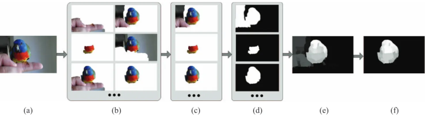
Fig. 2. Our proposal-based video saliency detection method. (a) Input frame. (b) Object proposals from the frame in (a). (c) Set of salient proposals are selected via a ranking strategy, which utilizes spatial saliency stimuli (Section III-A) and motion saliency cues (Section III-B). (d) Corresponding masks for salient proposals in (c). (e) We then transform these salient proposals (masks) into a saliency map by accounting for their pixel overlap. This voting procedure described in Section III-C effectively produces an initial saliency estimation. (f) Our final saliency result via an optimization process described in Section IV.

separately generating spatial and temporal saliency maps and then combining them into the spatiotemporal saliency maps. Fang et al. [29] merged the spatial and temporal saliency maps through an adaptive entropy-based uncertainty weight-ing approach. Kim et al. [18] obtained saliency maps at three different scales using the sum of absolute differences between temporal gradient maps and computed a weighted sum of the multiscale maps. In [30], a technique known as gradient flow was introduced for video saliency detection.

Some methods are based on the frequency domain, which focuses on extracting features of spectral domains. Guo et al. [23] employed the phase spectrum of the quater-nion Fourier transform (PQFT) to calculate spatiotemporal saliency for video frames. Kim and Kim [20] introduced textu-ral contrast into a multiscale framework, and used directional coherence as the orientation contrast to the temporal domain to retain the temporal consistency. A few of video saliency methods are based on the sparsity theory, which considers the small regions with high local contrast as meaningless noise. Hou and Zhang [24] decomposed the spatial and temporal tasks into a coding length increments task. Gao et al. [26] decomposed the matrices of temporally aligned video frames or robust principal component analysis into low-rank back-ground matrices and sparse salient object matrices.

Most of the methods referred above are based on pixel or superpixel level, e.g., Huang et al. [22] used the estimated key-points, Liu et al. [25] and Zhou et al. [19] proposed superpixel-based methods for spatio-temporal saliency calcu-lation. Whereas, in the case of multicomponent salient objects or cluttered backgrounds, these methods may not infer equal saliency values for the whole salient objects or backgrounds. Based on this observation, we build our approach on object-like regions, which compensates for the disadvantages of lacking object-level features in the previous works.

C. Object Proposal Segmentation

Object proposal methods, can output a set of image seg-ments once given an input image, which directly generates the object candidates that are likely to contain objects. The problem has received intensive interests in recent years [34]–[36], as it serves as an effective preprocessing

for other computer vision tasks such as unsupervised video segmentation [37]–[39], supervised object detection [40], and weakly supervised object localization [41]. Specifically, object proposals are extracted as a set of image segments, each of which is associated to a score encoding how likely it is to contain an object.

III. OBJECTPROPOSALS-BASED

SALIENCYDETECTION

An overview of our approach is presented in Fig. 2. The core premise of our algorithm is that salient object regions are identified from hundreds or thousands of object propos-als by considering several saliency cues at the object-level. For object proposals, a ranking scheme is designed to select salient object proposals based on spatial and temporal saliency cues [Fig. 2(c)]. Furthermore, a voting procedure is intro-duced to separate the foreground object regions from the background, which effectively produces an initial saliency esti-mation [Fig.2(d) and (e), SectionIII]. As shown in Fig.2(f), the initial saliency map is refined by considering object boundary refinement and temporal consistency to improve the accuracy of prediction in ambiguous regions (Section IV).

Let I= {I1,I2, . . .} be the set of input frames. For the tth

frame It, we apply the static region-ranking method to

gen-erate object proposal segmentations Pt = {p1_t,p2_t, . . .} [see Fig. 2(b)]. The proposals are generated via [34], and each frame would have hundreds of object candidates. Different from over-segmented regions, these proposal segments are more “object-like” as they have more distinct occlusion bound-aries and their appearances are in obvious contrast with nearby pixels. According to the objectness score from [34], which represents how likely a proposal is to contain an object, we select top 200 candidates for each frame. For each proposal pn_t in frame It, we compute a ranking score R(pnt) according

to spatial and temporal saliency cues, which is defined as R(pnt)=RF pnt +RMpnt (1) where RF and RM refer to intraframe visual saliency and motion saliency scores, respectively. Detailed descriptions of RF and RM are provided in SectionsIII-AandIII-B. We rank the proposals Ptaccording to their saliency scores R and select

Fig. 3. Saliency results generated by the top-ranked proposals with each individual prior score described in SectionIII. (a) Input frame. (b) Saliency results by the proposal background prior, which is generated by accumulating all the proposals with their background scores (3). (c) Saliency results by applying the center-surround contrast prior (4). (d) Saliency results only by considering motion contrast (7). (e) Saliency results by utilizing gradient summation (8). (f) Our initial saliency results by using the combination scores of all priors (11).

salient object proposals. In Section III-C, all the salient pro-posals are incorporated to obtain an initial saliency estimate via an overlap strategy.

A. Spatial Saliency Analysis

A number of saliency priors have been proposed for saliency detection, and the most widely used ones are the back-ground prior and center-surround contrast prior [8], [13], [31]–[33], [60]. However, in the previous works, both of these two priors are computed in low-level units, such as pixel or superpixel [47], [48], [54]. One obvious disadvan-tage is that they fail to treat the salient area as an entirety, since each prior only handles a fraction of the image. To compute an intraframe saliency score, we extend traditional low-level spatial saliency cues into the object level. We rede-fine the background prior and center-surround appearance contrast prior for object proposals. Furthermore, we incor-porate the objectness score from [34], which represents how likely a proposal is to contain a natural object, into our saliency estimates. Our spatial saliency score RF is formulated as

RFpn_t=Fobj pn_t+Fbg pn_t+Fcnt pn_t (2) where Fobj(pnt)indicates the objectness score of [34], which

has been obtained during the process of extracting object seg-mentation candidates. Fbg(pnt)and Fcnt(pnt) denote the

back-ground prior score and the center-contrast score, respectively. All three terms are normalized to [0, 1].

1) Proposal Background Prior: The background regions generally have a high probability of connecting with the image boundaries, which is known as the background prior. Zhu et al. [13] proposed a type of region-level background prior called boundary connectivity. Boundary connectivity is defined as the ratio of the perimeter of a region on the bound-ary to the square root of its area. However, as stated in [13], this measure might be difficult to compute on pixel or super-pixel level. This is due to boundary connectivity is based on object level or object segments and hard segmentation of image itself is a difficult and unsolved problem. Zhu et al. [13] used a soft formulation to compute boundary connectivity on superpixel level.

Fortunately, such an approach is naturally suitable for object proposals because the proposal represents a possible seg-ment of an object. Then, we introduce a proposal background prior score based on reorganized boundary connectivity, which encodes the assumption that the segments around image frame boundaries are more likely to belong to the background. The background prior score Fbg for proposal pnt is defined as

Fbg(pnt)=exp ⎛ ⎝₋pnt Bnd(It) Areapnt ⎞ ⎠ (3)

where Bnd(It) denotes the boundary pixels of frame It, and

Area(pnt) is the number of pixels in segment pnt. According

to this equation, if a proposal extensively touches the frame boundaries, it will be assigned by a higher background prior score, which indicates that it is less likely to be a salient object proposal.

As shown in Fig.2, the more this proposal connects to the boundaries, the higher probability it is assigned to the back-ground region. Even if the salient object is included in the proposal for some cases in Fig. 2(b), the background part of the proposal also occupies a larger ratio compared to the area of the entire proposal in the frame. Conversely, the border regions usually occupy a large area of the frame, thus there is an inverse relationship between the proposal’s background prior and its area. Saliency results according to the background prior are shown in Fig.3(b).

2) Proposal Center-Surround Contrast: Contrast prior-based saliency methods usually investigate the relationship between image regions and their neighborhoods. In our method, the proposal contrast measures the confidence that segment pnt represents the same object as its surroundings in

the video frame. To this end, we compute a CIELab color space histogram for proposal pn

t, and a 10-pixel dilated region

of pn_t as the neighboring region of the proposal. The contrast score Fcnt for proposal pnt is computed as

Fcnt pn_t=1−exp −χ2 Histc pn_t,Histc Dilpn_t (4) where Dil(pnt) denotes the dilated region of proposal pnt,

and χ2(pnt,Dil(pnt)) is the chi-squared distance between

L1-normalized appearance histograms. The saliency results using contrast score Fcnt can be seen in Fig.3(c).

B. Temporal Saliency Analysis

When dealing with video clips, motion provides a power-ful cue for saliency detection in addition to appearance. That is because pixels that abruptly change compared to their sur-roundings often attract more attention. We design a motion contrast-based saliency method. We first compute the optical flow using the large displacement optical flow method [45]. To obtain more robust motion information, we smoothen the initial optical-flow maps over the temporal domain. We then formulate our motion saliency score as

RMpn_t=Mbg pn_t+Mgrd pn_t+Mcnt pn_t (5) where Mbg is a motion contrast score, Mgrd is an optical-flow

gradient-based score, and Mcntrepresents a motion consistency

score. Saliency results using motion score RM are illustrated in Fig.3(d).

1) Smoothing Optical-Flow: Salient objects may not always move throughout the entire sequence. Unfortunately, a static object will cause discontinuities and inaccuracies in the standard optical-flow. To preserve temporal continuity and obtain a more robust optical-flow estimation, we make use of a Gaussian filter G that temporally smoothes the optical-flow estimate ot in frame It via

ot= l i₌₋lG(i;0,1)×ot+i l i=−lot+i (6) where l indicates the number of adjacent frames considered in this smooth process.

2) Motion Contrast-Based Saliency: The motion patterns of foreground objects and the background are usually different. We design a motion background contrast score Mbg(pnt) that

models this observation. A proposal, whose background prior score Fbgcomputed via (3) is less than e−1, will be treated as

background. Based on this, we compute the motion contrast between each proposal and the background proposals BP.

Specifically, given the smoothed optical flow ot = (u,v)

between two consecutive frames Itand It+1, the motion

distri-bution of proposal pn_t is encoded by two descriptors: a normal-ized histogram of the flow magnitude ograd=grad(√u2_+v2_),

and the distribution of flow orientation oori = arctan(v/u). Based on the histogram Histf of motion feature flow =

{ograd,oori}, we compute the motion contrast score Mbg for

proposal pnt with Mbg pnt =1−exp −χ2 Histflow pnt ,Histflow(BP) . (7)

Note that this score relies on relative motion, thus it can be applied to scenarios with a moving camera.

3) Motion Gradient Summation: The rationale behind motion contrast is that the motion pattern of an object is distinct from that of the background. This assumption can also be exploited via the gradient of the optical-flow. Indeed, distinct motion patterns cause velocity and orientation discon-tinuities. That is, the optical-flow gradient will be large around the salient object boundary. Therefore, we compute a motion gradient score Mgrd(pnt)by making use of the motion gradient

summation technique in [39]. This score is defined as the aver-age Frobenius norm of optical flow gradient in the boundary

of object proposal pn_t Mgrd(pnt)= otF= i₌x_,y j₌x_,y _{μi, υj}2 =μ2 x+μ2y+υx2+υx2 (8)

where ot =(μ, υ)is the smoothed optical flow of consecutive

frames It and It+1, μx, and μy are optical flow gradients in

the x direction and υx andυy are those in the y direction.

According to the definition of the motion gradient score, the higher value a pixel is, the greater the possibility it asso-ciates with moving salient object boundary. Actually, due to the approximation of optical flow computation, the gradient of optical flow cannot correspond to magnitude values in the boundaries of a moving object exactly. Therefore, we compare the average optical-flow gradient magnitude at the proposal boundary and in a dilated version of this boundary (10 pixels). The saliency results using the optical-flow gradient magnitude are shown in Fig.3(e).

4) Object Proposal Consistency: It is clear that salient object regions are consistent over time. Therefore, proposals corresponding to salient objects should also remain temporally consistent in adjacent frames. We define an interframe score for each proposal pn_t in frame It, based on the salient proposals

of the previous frame. Specifically, each object proposal pn_t−1 for frame It−1 can be warped to frame It according to the

forward optical flow. We then estimate the overlap between proposal pnt in frame It and the warped object proposals. This

yields the temporal consistency score Mcnt Mcnt pn_t= pˆ n t₋1 pnt Areapnt (9)

wherepˆn_t−1denotes the warped regions of the proposal pn t from

frame t−1 to frame t according to optical flow ot. Based on this

function, fractional proposals corresponding to the background should be filtered out, while object proposals should remain consistent over time.

Some co-saliency methods also infer the correspondence between regions, such as [53], [55], and [59]. However, we explore the relationship among object proposals in time axis, instead of inferring the semantic or interclass correspondence.

C. Voting for Saliency

Given the different saliency scores described above, we can compute a ranking score R(pn_t)for each proposal pn_t according to (1). For each frame It, we define the set of salient object

proposals as the 20% of proposals with the highest ranking scores. We define PSt ⊂Ptas the subset of such high-rank

pro-posals, and m as the number of salient object proposals in PSt.

To transform the salient proposal subset to a saliency map, we propose a voting scheme for inferring the saliency. A binary mask Mit is generated for salient proposal pit ∈ PSt, where

Mi

t(x)=1 if pixel x in frame It belongs to proposal pit, and 0

otherwise. For each pixel x, we compute the saliency value by accumulating the binary masks of the selected proposals PS

which is computed Ot(x)= 1 m i Mi t(x). (10)

We further normalize this value to obtain our initial saliency estimation as SIni_t (x)=1−exp −Ot(x) σ2 (11) where σ is a constant parameter for normalizing the ini-tial saliency maps. We validate the range of parameters in SectionV-B and set it asσ =3 through our experiments.

Examples of our initial saliency results are shown in Figs. 3(f) and 4(b). We can find that the foreground and background regions are clearly separated.

IV. SPATIOTEMPORALSALIENCYREFINEMENT

Although this initial saliency is relatively accurate, some ambiguities appear at the boundary of objects and temporal consistency is unsatisfactory. We now introduce a saliency refinement process to further improve our saliency estimates. A. Object Boundary Refinement

Our first goal is to refine the saliency map to obtain more accurate object boundaries. To this end, we first apply SLIC [49] to extract superpixels Rt = {r1t,r2t, . . .}from frame

It (about 500 superpixels for each frame). The initial saliency

SIni_t (ri_t)of superpixel ri_t is computed as the averaged saliency value of its pixels. Then superpixels Rtare separated into three

distinct parts: 1) foreground (salient) regions Ft; 2) background

(nonsalient) regions Bt; and 3) uncertain regions Ut Ft= rtf |SInit rft > τhigh_,∀ rtf ∈Rt Bt= r_tb|SIni_t rb_t < τlow_{, ∀r}b t ∈Rt Ut=Rt−Ft−Bt (12)

where two thresholds τhigh and τlow are set at 0.8 and 0.2, respectively. The detailed discussion of these two thresholds are presented in Section V-B. We then follow a graph-based approach to refine the saliency value of the uncertain regions. Specifically, for each frame It, we build an undirected

weighted graph using superpixels as nodes. This graph con-tains an edge between any two adjacent superpixels (rit,r

j t),

with the weight defined as the Euclidean distance between features encoding the average CIELab color space and the mean optical-flow magnitude. Furthermore, we compute the geodesic distance dgeo(rit,r

j

t) between any two superpixels

using the methods in [4] and [51]. We then add edges between any two background superpixels and any two foreground superpixels, with the weight set as zero. The saliency value of each uncertain superpixel ru

t ∈Ut is then defined as SRef_t r_tu=1−exp −max rft∈Ft dgeo ru_t,rft × min rbt∈Bt dgeo r_tu,r_tb . (13)

The rationale behind this equation is that the uncertain area ru

t should have a high saliency probability when it differs from

Fig. 4. Example of the spatiotemporal saliency refinement process. (a) Original video frames of Girl from SegTrack, with the frames ordered according to time. (b) Initial saliency maps obtained via our object-based saliency detection described in Section III. (c) Results of saliency refine-ment (Section IV-A). (d) Final results exploiting temporal consistency (SectionIV-B).

the background superpixels and is close to the foreground ones. Fig. 4(c) shows an example of the resulting saliency maps. It can be seen that the arms and legs of the Girl are successfully highlighted.

B. Temporal Saliency Consistency

In order to further improve the temporal consistency of the refined saliency estimates SRef, we introduce a propagation process as in [52] to propagate the per-frame saliency maps over time. For the first frame I1, the location prior is initialized

with the refined proposal saliency map SRef₁ . For the following frames, the saliency value of superpixel rj is computed as:

SFin_t+1 r_tj₊₁ = iφ rit,r j t+1 ·ψrti iφ rit,r j t+1 SRef_t ri_t with ψrit =exp −ogradrit (14) where φ(ri t,r j

t+1) indicates the overlap between superpixel ri

t warped by optical-flow and superpixel r j

t+1, and ograd is

the same normalized histogram of flow magnitude as used in Section III-B to compute the motion contrast score. This process is performed as independent forward and backward propagation steps, and the final result is the mean value of these two steps. The results of the Girl example are shown in Fig.4(d), where the saliency results are more accurate.

V. EXPERIMENTALRESULTS

The proposed object proposals-based video saliency method automatically detects salient objects in video sequences. We demonstrate the benefits of our approach on three benchmark datasets and provide quantitative and qualitative comparisons with nine state-of-the-art methods. We use the implementa-tions provided by the authors of these methods and set their free parameters so as to maximize their performance. A. Experimental Settings

1) Datasets: We first evaluate our method on the SegTrackV2 dataset [58], which is an updated version of the SegTrack dataset [56] with full pixel-level ground-truth (GT)

annotations on multiple objects in each frame. The updated SegTrackV2 dataset totally introduces 14 sequences (Birdfall, Cheetah, Girl, Monkeydog, Parachute, Penguin, Drifting Car, Hummingbird, Frog, Worm, Soldier, Monkey, Bird of Paradise, and BMX) that presents different challenges. We also evaluate our approach on the well-known Freiburg–Berkeley Motion Segmentation Dataset (FBMS) [44]. Finally, we challenge the current Densely Annotated Video Segmentation (DAVIS) dataset [7], which is designed for the task of video object segmentation with 50 video clips with the binary labels.

2) Comparison Methods: We compare our approach with three image saliency methods, frequency-tuned saliency (IG) [11], saliency filter (SF) [5], and low rank (LR) [1], and with six well-known video saliency techniques, self resem-blance saliency detection (SD) [43], PQFT [23], space-time saliency (TM) [19], gradient flow video saliency (GFS) [30], and saliency-aware geodesic segmentation (SG) [4], video saliency via spatiotemporal cues and uncertainty weighting (US) [29].

3) Evaluation Metrics: We report the precision versus recall curves (PR curves), F-score curves, and mean absolute errors (MAEs) for evaluation. The precision value represents the ratio of correctly assigned salient pixels to all the pixels in the detected regions, while the recall rate is the percentage of detected regions among the true positive samples. The curves are averaged over each video sequence. The F-measure in [11], considers both precision and recall, and can be computed as

F_β = (1+β

2_{)·Precision·Recall}

β2_{·Precision+Recall} . (15)

We set β2 = 0.3 throughout our experiments. The MAE in [5], is defined between a saliency map S and the binary GT as MAE = (1/|I|)_x|S(x)−GT(x)| , where |I| represents the number of pixels and x stands for all image pixels. B. Parameter Validation

The optimal parameter settings are used to achieve the best performance considering the precision and MAE measures on SegTrackV2 [58], FBMS [44], and DAVIS [7] datasets com-prehensively. For the optical-flow and proposal segmentation calculations in our method, we set the source codes as default parameter settings provided by the authors, and the detailed settings are referred to [34] and [44].

Fig.5 shows some important parameter settings mentioned in our method. In Fig. 5(a), we use the MAE measure to describe the ratio of the number of voted top-ranked propos-als in SectionIII-C. Voting too many proposals may introduce more inaccurate proposals, which will negatively impact the performance of the initial saliency estimate. While less voting candidates tend to neglect several parts of the salient object, then it is likely to lose the completeness of the detection. We run each ratio of the set of salient object proposals for ranking scores, and select top 20% of proposals with the highest rank-ing scores. In Fig. 5(b), we use the precision rates of initial saliency results to define two thresholds which separate fore-ground and backfore-ground thresholds in (12). With the increase of the threshold, the precision of the initial saliency map gets

(a) (b)

(c) (d)

Fig. 5. Validation of the parameters used in our method. (a) Ratio of the num-ber of voted top-ranked proposals in SectionIII-C. (b) Evaluates the selection strategy of two thresholdsτlowandτhighwhich separate initial saliency maps into foreground and background parts (12). (c) Illustrates the number of adja-cent frames of smoothing optical-flow involved in SectionIII-B1. (d) Constant parameter ofσ in (11).

lower. Moreover, the precision decreases rapidly when we set the precision value τlow = 0.2. Similarly, when the thresh-old exceeds the background threshthresh-old τhigh =0.8, the value of gradient flow will level off. Fig. 5(c) illustrates the num-ber of adjacent frames of smoothing optical-flow involved in SectionIII-B1. Having a larger neighboring system for a cer-tain frame, long-range motion information will be taken into account, thus ignoring some unreliable optical flow estima-tion. However, this possibly makes optical flow unreliable and loses discriminative ability. When the number of adjacent frames decreases, only considering the motion information of few frames will be influenced by inaccurate optical flow estimation. We set the number of adjacent frames as l = 5 in (6). Fig. 5(d) shows the setting of the constant parame-ter of σ in (11), which determines the relative contrast of initial saliency maps. We report the performance by varying σ = {0.5,1,2,3,4,5}withσ =3 in our implementation. C. Comparison on SegTrackV2

The results for experiments on SegTrackV2 [58] are shown in Fig. 6. The PR curve (first column) and F-measure curve (second column) of our method are clearly above baselines, which indicates that our predicted saliency values are clos-est to the GT. Similarly, we obtain a lower MAE value (third column) than the baselines, indicating higher accuracy of our method. In particular, our MAE value of 0.0426 in SegTrackV2 is significantly lower than that of the second

Fig. 6. Comparison of PR curves (left), F-measure curves (middle), and MAE measurements (right) on the SegTrackV2 dataset [58].

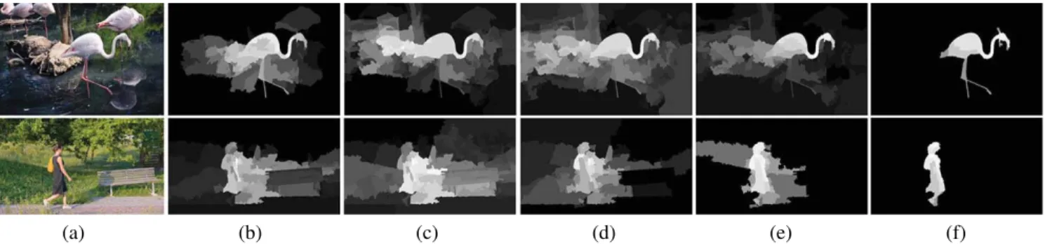
Fig. 7. Visual comparison of previous approaches with our method and with GT on SegTrackV2. From left to right: representative frames of the input videos, GT, our method, GFS [30], SG [4], IG [11], SF [5], SD [43], PQFT [23], and TM [19].

best method (SG [4] in this case). Some qualitative compar-ison is shown in Fig. 7, and they clearly show the benefits of our approach. Our saliency maps accurately highlight the outline of the salient object thanks to object-level compu-tation. Furthermore, due to our proposal selection process, background noise is significantly reduced. Importantly, our proposal-based saliency maps can even filter out cluttered background regions.

In contrast, IG [11], SF [5], and LR [1] work with still images. IG [11] exploits spatial frequencies to compute saliency using color and lightness properties. SF [5] estimates saliency from uniqueness and spatial distribution, which are two important measurements in contrast-based approaches. LR [1] models the background regions of the image as the low-rank matrix, and the salient regions are treated as sparse noises. While they all yield good results, they suffer from their lack of motion information. As a consequence, they often fail to accurately locate fast-moving objects. For instance, in the

Cheetah sequence, the background is cluttered, and the fore-ground object does not stand out on appearance alone, which represents a difficult scenario for these methods.

In contrast, GFS [30], SG [4], SD [43], PQFT [23], TM [19], and US [4] make use of additional motion features to detect spatiotemporally salient objects. GFS [30], based on the gra-dient flow field and energy optimization, estimates salient regions in videos. The proposed effective utilization of gra-dient flow field information is robust to estimating the object and background in complex scenes. SG [4] integrates spa-tiotemporal edge maps and geodesic distances to compute spatiotemporal saliency. The spatiotemporal edge maps con-sist of spatial static edges within the same frame and motion boundary edges estimated from neighboring frames. In Fig.7, SG tends to produce blurred object boundaries (Bird of Paradise). SD [43] is a bottom-up approach that computes local regression kernels as local descriptors to measure the likeness of a pixel or voxel to its surroundings. In most

Fig. 8. Comparison of PR curves (left), F-measure curves (middle), and MAE measurements (right) on the FBMS dataset [44].

Fig. 9. Visual comparison of previous approaches with our method and with GT on FBMS [44]. From left to right: representative frames of the input videos, GT, our method, GFS [30], SG [4], IG [11], SF [5], SD [43], PQFT [23], and TM [19].

cases, SD can locate salient objects by accounting for tem-poral information, but the saliency maps are low resolution and some moving objects are assigned low saliency values (Monkeydog). In PQFT [23], the motion features are com-bined into a PQFT process to obtain spatiotemporal saliency maps. However, this method only focuses on very local content without highlighting the entire object (Monkeydog). The spa-tiotemporally salient object estimation of TM [19] is based on feature contrast and local priors. However, this method fails to take the temporal coherence of the saliency map across the video into consideration. Another limitation is that, for complex motion patterns, the original contrast-based features cannot correctly locate salient objects.

D. Comparison on FBMS Dataset

Results of our experiments on the FBMS dataset [44] are shown in Fig.8. The PR curve (first column) and F-measure curve (second column) indicate that our method again achieves better performance than the other tested methods. We obtain the lowest MAE value (third column) compared to baselines. In FBMS, our method obtains an MAE of 0.0495, which

is lower than that of other state-of-the-art saliency detec-tion methods and indicates superior accuracy. Fig. 9 shows some comparison results using our method and other methods. The compared methods exhibit the drawback of the dark-ness in the center of the salient object and a discontinuous shape of the object. Our proposal selection process retains the objectness of the salient object and decreases the noise from cluttered backgrounds. IG [11] and SF [5] could not precisely locate the salient object due to the lack of motion information, and they underperformed due to the similarity appearance of the foreground and background. For instance, in the cars sequences, these two methods simply treated the brightest region as the salient region, where their performance was limited with complex scenes (cats and farm).

SG [4], SD [43], PQFT [23], and TM [19] were able to locate the salient objects from the motion information but also suffered from various drawbacks. SG [4] produced darkness in the center of the salient object (farm) because the method is calculated at the superpixel scale, a common problem with superpixel-based methods. SD [43] and PQFT [23] showed blurred object boundaries (farm), due to the failure to preserve the semantic information of the object. Furthermore, the

Fig. 10. Comparison of PR curves (left), F-measure curves (middle), and MAE measurements (right) on the DAVIS dataset [7].

Fig. 11. Visual comparison of previous approaches with our method and with GT on DAVIS [7]. From left to right: representative frames of the input videos, GT, our method, GFS [30], SG [4], IG [11], SF [5], SD [43], PQFT [23], and TM [19].

temporal coherence was not maintained very well (rabbits). TM [19] sometimes obtained the entire salient object mask (rabbits and cats), but the complex color distributions and high similarity between the foreground and background made it difficult to locate the salient object and the noisy background phenomenon persisted in some cases (farm).

E. Comparison on DAVIS Dataset

We also test our method on the DAVIS dataset [7]. The quantitative and qualitative results are shown in Figs. 10 and 11. We obtain an MAE of 0.0884 in DAVIS dataset. As demonstrated in Fig. 11, our proposal selection process retains the completeness of the salient object and decreases the noise from cluttered backgrounds. Compared to other methods, the saliency detection methods IG [11], SF [5], SD [43], and PQFT [23] were not able to show the accurate location of the salient object because of the lack of motion information (bear and rollerblade). SG [4] and GFS [30] were able to locate the salient objects with monotonous appearance (bear and car-shadow), but did not well on objects with various appearance

(rollerblade). TM [19] mainly outputs noisy in background regions because of the clustered background (car-shadow). F. Algorithm Validation

The runtime of the proposed algorithm costs 8.36 s for a typical 320×420 frame, including average time of 3.92 s for generating initial saliency map, 3.12 s for boundary refinement and 1.32 s for temporal consistency calculation. The run-time excludes the optical-flow computation and the proposal extraction process, which are used as input. Our method can locate salient objects with complex motion patterns, and high-light more complete foreground objects than state-of-the-art methods. Furthermore, our algorithm incorporates intraframe saliency and motion cues and clearly distinguishes moving salient objects from the background.

VI. CONCLUSION

We have presented a novel approach to video saliency detec-tion using object proposals. Our overall aim was to make full use of object-level representations such as object proposals to

further improve video salient object detection models. We fol-lowed a more intuitive approach at the object level. Rather than individually calculating saliency values at small scales, our method directly located candidate salient object proposals via a more intuitive visual saliency analysis. Compared to the state-of-the-art methods, our method accurately located com-plete salient objects with complex motion patterns, even in the presence of cluttered background. In our future work, we will pay attention to extending this paper for stereo saliency detection tasks (e.g., [60]) and event-driven studies (e.g., [62]).

REFERENCES

[1] X. Shen and Y. Wu, “A unified approach to salient object detection via low rank matrix recovery,” in Proc. IEEE CVPR, Providence, RI, USA, 2012, pp. 853–860.

[2] H. Kim, Y. Kim, J.-Y. Sim, and C.-S. Kim, “Spatiotemporal saliency detection for video sequences based on random walk with restart,” IEEE Trans. Image Process., vol. 24, no. 8, pp. 2552–2564, Aug. 2015. [3] J. Peng, J. Shen, and X. Li, “High-order energies for stereo

segmenta-tion,” IEEE Trans. Cybern., vol. 46, no. 7, pp. 1616–1627, Jul. 2016. [4] W. Wang, J. Shen, and F. Porikli, “Saliency-aware geodesic video

object segmentation,” in Proc. IEEE CVPR, Boston, MA, USA, 2015, pp. 3395–3402.

[5] F. Perazzi, P. Krähenbühl, Y. Pritch, and A. Hornung, “Saliency fil-ters: Contrast based filtering for salient region detection,” in Proc. IEEE CVPR, Providence, RI, USA, 2012, pp. 733–740.

[6] Q. Zhang, Y. Liu, S. Zhu, and J. Han, “Salient object detection based on super-pixel clustering and unified low-rank representation,” Comput. Vis. Image Understand., vol. 161, pp. 51–64, Aug. 2017.

[7] F. Perazzi et al., “A benchmark dataset and evaluation methodology for video object segmentation,” in Proc. IEEE CVPR, Las Vegas, NV, USA, 2016, pp. 724–732.

[8] M.-M. Cheng, N. J. Mitra, X. Huang, P. H. S. Torr, and S.-M. Hu, “Global contrast based salient region detection,” IEEE Trans. Pattern Anal. Mach. Intell., vol. 37, no. 3, pp. 569–582, Mar. 2015.

[9] J. Shen, D. Wang, and X. Li, “Depth-aware image seam carving,” IEEE Trans. Cybern., vol. 43, no. 5, pp. 1453–1461, Oct. 2013.

[10] D. Gao, S. Han, and N. Vasconcelos, “Discriminant saliency, the detec-tion of suspicious coincidences, and applicadetec-tions to visual recognidetec-tion,” IEEE Trans. Pattern Anal. Mach. Intell., vol. 31, no. 6, pp. 989–1005, Jun. 2009.

[11] R. Achanta, S. Hemami, F. Estrada, and S. Susstrunk, “Frequency-tuned salient region detection,” in Proc. IEEE CVPR, Miami, FL, USA, 2009, pp. 1597–1604.

[12] Q. Wang, Y. Yuan, and P. Yan, “Visual saliency by selective contrast,” IEEE Trans. Circuits Syst. Video Technol., vol. 23, no. 7, pp. 1150–1155, Jul. 2013.

[13] W. Zhu, S. Liang, Y. Wei, and J. Sun, “Saliency optimization from robust background detection,” in Proc. IEEE CVPR, Columbus, OH, USA, 2014, pp. 2814–2821.

[14] Q. Wang, P. Yan, Y. Yuan, and X. Li, “Multi-spectral saliency detection,” Pattern Recognit. Lett., vol. 34, no. 1, pp. 34–41, 2013.

[15] Q. Wang, Y. Yuan, P. Yan, and X. Li, “Saliency detection by multiple-instance learning,” IEEE Trans. Cybern., vol. 43, no. 2, pp. 660–672, Apr. 2013.

[16] Q. Wang, G. Zhu, and Y. Yuan, “Multi-spectral dataset and its application in saliency detection,” Comput. Vis. Image Understand., vol. 117, no. 12, pp. 1748–1754, 2013.

[17] D. Gao, V. Mahadevan, and N. Vasconcelos, “The discriminant center-surround hypothesis for bottom-up saliency,” in Proc. NIPS, 2007, pp. 497–504.

[18] W. Kim, C. Jung, and C. Kim, “Spatiotemporal saliency detection and its applications in static and dynamic scenes,” IEEE Trans. Circuits Syst. Video Technol., vol. 21, no. 4, pp. 446–456, Apr. 2011.

[19] F. Zhou, S. B. Kang, and M. F. Cohen, “Time-mapping using space-time saliency,” in Proc. IEEE CVPR, Columbus, OH, USA, 2014, pp. 3358–3365.

[20] W. Kim and C. Kim, “Spatiotemporal saliency detection using textural contrast and its applications,” IEEE Trans. Circuits Syst. Video Technol., vol. 24, no. 4, pp. 646–659, Apr. 2014.

[21] J. Li, Y. Tian, T. Huang, and W. Gao, “Probabilistic multi-task learning for visual saliency estimation in video,” Int. J. Comput. Vis., vol. 90, no. 2, pp. 150–165, 2010.

[22] C.-R. Huang, Y.-J. Chang, Z.-X. Yang, and Y.-Y. Lin, “Video saliency map detection by dominant camera motion removal,” IEEE Trans. Circuits Syst. Video Technol., vol. 24, no. 8, pp. 1336–1349, Aug. 2014. [23] C. Guo, Q. Ma, and L. Zhang, “Spatio-temporal saliency detection using phase spectrum of quaternion Fourier transform,” in Proc. IEEE CVPR, Anchorage, AK, USA, 2008, pp. 1–8.

[24] X. Hou and L. Zhang, “Dynamic visual attention: Searching for coding length increments,” in Proc. NIPS, 2008, pp. 681–688.

[25] Z. Liu, X. Zhang, S. Luo, and O. Le Meur, “Superpixel-based spatiotem-poral saliency detection,” IEEE Trans. Circuits Syst. Video Technol., vol. 24, no. 9, pp. 1522–1540, Sep. 2014.

[26] Z. Gao, L.-F. Cheong, and Y.-X. Wang, “Block-sparse RPCA for salient motion detection,” IEEE Trans. Pattern Anal. Mach. Intell., vol. 36, no. 10, pp. 1975–1987, Oct. 2014.

[27] T. H. Kim, K. M. Lee, and S. U. Lee, “Generative image segmentation using random walks with restart,” in Proc. ECCV, 2008, pp. 264–275. [28] V. Mahadevan and N. Vasconcelos, “Spatiotemporal saliency in dynamic

scenes,” IEEE Trans. Pattern Anal. Mach. Intell., vol. 32, no. 1, pp. 171–177, Jan. 2010.

[29] Y. Fang, Z. Wang, W. Lin, and Z. Fang, “Video saliency incorporat-ing spatiotemporal cues and uncertainty weightincorporat-ing,” IEEE Trans. Image Process., vol. 23, no. 9, pp. 3910–3921, Sep. 2014.

[30] W. Wang, J. Shen, and L. Shao, “Consistent video saliency using local gradient flow optimization and global refinement,” IEEE Trans. Image Process., vol. 24, no. 11, pp. 4185–4196, Nov. 2015.

[31] J. Han et al., “Background prior-based salient object detection via deep reconstruction residual,” IEEE Trans. Circuits Syst. Video Technol., vol. 25, no. 8, pp. 1309–1321, Aug. 2015.

[32] J. Han et al., “Two-stage learning to predict human eye fixations via SDAEs,” IEEE Trans. Cybern., vol. 46, no. 2, pp. 487–498, Feb. 2016. [33] J. Han, E. J. Pauwels, and P. de Zeeuw, “Fast saliency-aware multi-modality image fusion,” Neurocomputing, vol. 111, no. 6, pp. 70–80, 2013.

[34] I. Endres and D. Hoiem, “Category independent object proposals,” in Proc. ECCV, 2010, pp. 575–588.

[35] J. Carreira and C. Sminchisescu, “Constrained parametric min-cuts for automatic object segmentation,” in Proc. IEEE CVPR, San Francisco, CA, USA, 2010, pp. 3241–3248.

[36] B. Alexe, T. Deselaers, and V. Ferrari, “What is an object?” in Proc. IEEE CVPR, 2010, pp. 73–80.

[37] Y. J. Lee, J. Kim, and K. Grauman, “Key-segments for video object segmentation,” in Proc. IEEE ICCV, Barcelona, Spain, 2011, pp. 1995–2002.

[38] T. Ma and L. J. Latecki, “Maximum weight cliques with mutex constraints for video object segmentation,” in Proc. IEEE CVPR, Providence, RI, USA, 2012, pp. 670–677.

[39] D. Zhang, O. Javed, and M. Shah, “Video object segmentation through spatially accurate and temporally dense extraction of primary object regions,” in Proc. IEEE CVPR, Portland, OR, USA, 2013, pp. 628–635. [40] R. Girshick, J. Donahue, T. Darrell, and J. Malik, “Rich feature hierar-chies for accurate object detection and semantic segmentation,” in Proc. IEEE CVPR, Columbus, OH, USA, 2014, pp. 580–587.

[41] R. G. Cinbis, J. Verbeek, and C. Schmid, “Multi-fold MIL training for weakly supervised object localization,” in Proc. IEEE CVPR, Columbus, OH, USA, 2014, pp. 2409–2416.

[42] J. Shen, X. Yang, Y. Jia, and X. Li, “Intrinsic images using optimization,” in Proc. IEEE CVPR, Colorado Springs, CO, USA, 2011, pp. 3481–3487.

[43] H. J. Seo and P. Milanfar, “Static and space-time visual saliency detection by self-resemblance,” J. Vis., vol. 9, no. 12, pp. 1–27, 2009. [44] T. Brox and J. Malik, “Object segmentation by long term analysis of

point trajectories,” in Proc. ECCV, 2010, pp. 282–295.

[45] T. Brox and J. Malik, “Large displacement optical flow: Descriptor matching in variational motion estimation,” IEEE Trans. Pattern Anal. Mach. Intell., vol. 33, no. 3, pp. 500–513, Mar. 2011.

[46] X. Dong et al., “Occlusion-aware real-time object tracking,” IEEE Trans. Multimedia, vol. 19, no. 4, pp. 763–771, Apr. 2017.

[47] X. Dong, J. Shen, L. Shao, and L. Van Gool, “Sub-Markov random walk for image segmentation,” IEEE Trans. Image Process., vol. 25, no. 2, pp. 516–527, Feb. 2016.

[48] J. Shen et al., “Real-time superpixel segmentation by DBSCAN clus-tering algorithm,” IEEE Trans. Image Process., vol. 25, no. 12, pp. 5933–5942, Dec. 2016.

[49] R. Achanta et al., “SLIC superpixels compared to state-of-the-art super-pixel methods,” IEEE Trans. Pattern Anal. Mach. Intell., vol. 34, no. 11, pp. 2274–2282, Nov. 2012.

[50] W. Wang, J. Shen, X. Li, and F. Porikli, “Robust video object coseg-mentation,” IEEE Trans. Image Process., vol. 24, no. 10, pp. 3137–3148, Oct. 2015.

[51] X. Bai and G. Sapiro, “A geodesic framework for fast interactive image and video segmentation and matting,” in Proc. IEEE ICCV, 2007, pp. 1–8.

[52] A. Papazoglou and V. Ferrari, “Fast object segmentation in uncon-strained video,” in Proc. IEEE ICCV, Sydney, NSW, Australia, 2013, pp. 1777–1784.

[53] D. Zhang, J. Han, J. Han, and L. Shao, “Cosaliency detection based on intrasaliency prior transfer and deep intersaliency mining,” IEEE Trans. Neural Netw. Learn. Syst., vol. 27, no. 6, pp. 1163–1176, Jun. 2016. [54] J. Shen, Y. Du, W. Wang, and X. Li, “Lazy random walks for

super-pixel segmentation,” IEEE Trans. Image Process., vol. 23, no. 4, pp. 1451–1462, Apr. 2014.

[55] D. Zhang, J. Han, C. Li, J. Wang, and X. Li, “Detection of co-salient objects by looking deep and wide,” Int. J. Comput. Vis., vol. 120, no. 2, pp. 215–232, 2016.

[56] D. Tsai, M. Flagg, A. Nakazawa, and J. M. Rehg, “Motion coher-ent tracking using multi-label MRF optimization,” Int. J. Comput. Vis., vol. 100, no. 2, pp. 190–202, 2012.

[57] W. Wang, J. Shen, and F. Porikli, “Selective video object cutout,” IEEE Trans. Image Process., vol. 26, no. 12, pp. 5645–5655, Dec. 2017. [58] F. Li, T. Kim, A. Humayun, D. Tsai, and J. M. Rehg, “Video

segmen-tation by tracking many figure-ground segments,” in Proc. IEEE ICCV, Sydney, NSW, Australia, 2013, pp. 2192–2199.

[59] X. Yao, J. Han, D. Zhang, and F. Nie, “Revisiting co-saliency detection: A novel approach based on two-stage multi-view spectral rotation co-clustering,” IEEE Trans. Image Process., vol. 26, no. 7, pp. 3196–3209, Jul. 2017.

[60] J. Han, L. Shao, D. Xu, and J. Shotton, “Enhanced computer vision with microsoft kinect sensor: A review,” IEEE Trans. Cybern., vol. 43, no. 5, pp. 1318–1334, Oct. 2013.

[61] W. Wang, J. Shen, and L. Shao, “Video salient object detection via fully convolutional networks,” IEEE Trans. Image Process., to be published, doi:10.1109/TIP.2017.2754941.

[62] D. Zhang, J. Han, L. Jiang, S. Ye, and X. Chang, “Revealing event saliency in unconstrained video collection,” IEEE Trans. Image Process., vol. 26, no. 4, pp. 1746–1758, Apr. 2017.

Fang Guo is currently pursuing the Ph.D. degree

with the School of Computer Science, Beijing Institute of Technology, Beijing, China.

Her current research interest includes learning-based saliency detection methods.

Wenguan Wang is currently pursuing the Ph.D.

degree with the School of Computer Science, Beijing Institute of Technology, Beijing, China.

His current research interests include object detec-tion and segmentadetec-tion for images and videos.

Jianbing Shen (M’11–SM’12) is a Professor with the School of Computer Science, Beijing Institute of Technology, Beijing, China. He has published about 70 journal and conference papers, such as the IEEE TRANSACTIONS ON PATTERN

ANALYSIS AND MACHINE INTELLIGENCE, the IEEE TRANSACTIONS ONCYBERNETICS, and the IEEE TRANSACTIONS ON IMAGE PROCESSING. His current research interests include computer vision and multimedia processing.

Mr. Shen was a recipient of several flagship hon-ors, including the Fok Ying Tung Education Foundation from the Ministry of Education, the Program for Beijing Excellent Youth Talents from the Beijing Municipal Education Commission, and the Program for New Century Excellent Talents from the Ministry of Education. He is on the Editorial Board of Neurocomputing.

Ling Shao (M’09–SM’10) received the Ph.D. degree

in computer vision from the University of Oxford, Oxford, U.K.

He is a Professor with the School of Computing Sciences, University of East Anglia, Norwich, U.K. His current research interests include computer vision, pattern recognition, and machine learning.

Dr. Shao is an Associate Editor of the IEEE TRANSACTIONS ON IMAGE PROCESSING, the IEEE TRANSACTIONS ON NEURAL NETWORKS ANDLEARNINGSYSTEMS, and other journals.

Jian Yang received the Ph.D. degree in optical

engi-neering from the Beijing Institute of Technology, Beijing, China, in 2007.

He is currently a Full Professor with the School of Optoelectronics, Beijing Institute of Technology. His current research interests include medical image processing and augmented reality.

Dacheng Tao (F’15) is a Professor of computer

science and an ARC Laureate Fellow with the School of Information Technologies and the Faculty of Engineering and Information Technologies, and the Inaugural Director of the UBTECH Sydney Artificial Intelligence Centre, University of Sydney, Darlington, NSW, Australia. He mainly applies statistics and mathematics to artificial intelligence and data science. His current research interests include computer vision, data science, image pro-cessing, machine learning, and video surveillance. Mr. Tao was a recipient of the 2015 Australian Scopus-Eureka Prize, and the 2015 ACS Gold Disruptor Award.

Yuan Yan Tang (F’04) is currently a Chair

Professor with the Faculty of Science and Technology, University of Macau, Macau, China. His current research interests include wavelets, pattern recognition, and image processing.

Dr. Tang is the Founder and the Editor-in-Chief of the International Journal of Wavelets, Multiresolution, and Information Processing. He is the Founder and the Chair of the Pattern Recognition Committee of the IEEE Systems, Man, and Cybernetics.