THE DEFORMED GRAPH LAPLACIAN AND ITS APPLICATIONS TO NETWORK CENTRALITY ANALYSIS
PETER GRINDROD∗, DESMOND J. HIGHAM†, ANDVANNI NOFERINI‡
Abstract. We introduce and study a new network centrality measure based on the concept of nonbacktracking walks; that is, walks not containing subsequences of the formuvuwhereu andv
are any distinct connected vertices of the underlying graph. We argue that this feature can yield more meaningful rankings than traditional walk-based centrality measures. We show that the result-ing Katz-style centrality measure may be computed via the so-called deformed graph Laplacian—a quadratic matrix polynomial that can be associated with any graph. By proving a range of new results about this matrix polynomial, we gain insights into the behavior of the algorithm with re-spect to its Katz-like parameter. The results also inform implementation issues. In particular we show that, in an appropriate limit, the new measure coincides with the nonbacktracking version of eigenvector centrality introduced by Martin, Zhang and Newman in 2014. Rigorous analysis on star and star-like networks illustrates the benefits of the new approach, and further results are given on real networks.
Keywords: Centrality index, deformed graph Laplacian, matrix polynomial, nonbacktracking, complex network, generating function.
MSC classification: 05C50, 05C82, 15A18, 15A54, 15B48, 15B99, 65F15 1. Introduction. Network science is producing a wide range of challenging re-search problems that have diverse applications across science and engineering. Many important questions in this area can be cast in terms of applied linear algebra. In particular, operating on networks leads us naturally into the rich and elegant field of matrix function theory. In this work, we consider network centrality measures, a topic where many tools have been developed and tested [19, 47]. We focus on walk-based centrality measures [12, 20, 22]. Here the aim is to identify influential nodes by quantifying their potential to disperse information along the network edges. A key novelty in our work is to ignore certain types of walk around the network that, in terms of quantifying centrality, have little relevance. The combinatorics of the remain-ing “nonbacktrackremain-ing walks” can be dealt with conveniently via a matrix polynomial representation, leading to an efficient computational algorithm. This viewpoint also allows us to raise and solve several new theoretical problems on this matrix polyno-mial, giving further insight into the algorithm.
In section2, we review some relevant material on walk-based centrality measures, focusing on Katz and eigenvector centrality. In section 3, we then motivate a new definition of centrality based on the concept of a nonbacktracking walk. We show on a simple star graph how restricting attention to nonbacktracking walks can avoid a localization issue. Section4provides some preliminary material on matrix polynomials and, in particular, sets up the so-called deformed graph Laplacian, which is the main object of study in our work, and derives some new basic connections between the eigenvalues of the deformed graph Laplacian and the features of the underlying graph. In section5, we consider the combinatorics of nonbacktracking walks, and show how an analogue of Katz centrality can be expressed in terms of the deformed graph Laplacian.
∗Mathematical Institute, University of Oxford, Andrew Wiles Building, Radcliffe Observatory
Quarter, Woodstock Road, Oxford, UK, OX2 6GG. ([email protected])
†Department of Mathematics and Statistics, University of Strathclyde, Glasgow, UK, G1
1XH. ([email protected]) Supported by EPSRC/RCUK Established Career Fellowship EP/M00158X/1 and by a Royal Society/Wolfson Research Merit Award.
‡Department of Mathematical Sciences, University of Essex, Wivenhoe Park, Colchester, UK,
Relevant properties of the deformed graph Laplacian are then studied in sections 6,
7, 8, 9 and 10. More specifically, sections 6 and 7 contain our main theoretical results, exploring further the spectral properties of the deformed graph Laplacian, and connecting them to the radius of convergence of a certain power series that generates the combinatorics of nonbacktracking walks. In section8we consider how to compute or bound the radius of convergence, and discuss other practical issues. Section 9
develops the relation between the deformed graph Laplacian and M-matrix theory. We show in section 10 that the nonbacktracking version of eigenvector centrality introduced by Martin, Zhang and Newman [33], which was derived from a different viewpoint, coincides with the nonbacktracking walk centrality in an appropriate limit. A large scale synthetic example is then analysed in section11, in order to shed further light on the new centrality measure, and tests on real data are given in section12. We finish in section13with a short summary.
It is worth mentioning that Theorem6.1and slightly weaker versions of Theorem
4.7 and Lemma 6.2 are not entirely new. They can also be obtained using purely graph theoretical techniques based on zeta funtions, namely, Theorem 2 in [43]. We opted, however, to include our own proofs based on matrix theory, as they allow us to prove stronger statements and present a self-contained treatment. We also emphasize that the other theoretical results in this paper are, to our knowledge, new.
2. Walk-based Centrality. We letA∈Rn×n denote the adjacency matrix of a simple, undirected graph, soaij = 1 if there is an edge from node ito nodej and aij = 0 otherwise. Awalk of length kis any sequence ofk+ 1 nodes,i1, i2, . . . , ik+1
such that each edgeir↔ir+1 is present in the network [11,14,19]. Loosely, a walk
is a traversal around the network in which nodes and edges may be re-used.
We may, of course, place further restrictions on the traversal—a trail must use distinct edges, apathmust use distinct nodes and ashortest pathmust use the smallest possible number of edges. Borgatti [11] discusses the relevance of these concepts with respect to processes that take place over a network, such as message-passing, disease-spreading and various types of business transaction. This variety of processes has led to a wide range of centrality measures that aim to summarize the importance of the network nodes through their ability to initiate traversals. We focus here on the case of walks for two main reasons. First, walks are relevant in many realistic circumstances, notably, where there is a stochastic element to the dynamics; for example, a fixed object such as a soccer ball, an office laptop or the keys to a company car may be passed arbitrarily around a well-defined interaction network. Second, and from a more practical perspective, walks are convenient to compute with, making it feasible to study the type of large-scale networks arising in modern applications.
A classic result from graph theory tells us that (Ak)ij counts the number of distinct walks of length k from i to j; see, for example, [14, Theorem 2.2.1]. Now, let ρ(A) denote the spectral radius of A and suppose 0 < α < ρ(A)−1. Then the
resolvent
(I−αA)−1=I+αA+α2A2+α3A3+· · · (2.1)
has ani, jelement that records a weighted sum of all walks1from itoj, with walks of lengthkdownweighted by the factorαk. Katz [28] suggested that the importance, or centrality, of node i could be quantified by summing this count over all such j,
1
leading to the linear system
(I−αA)x=1. (2.2)
Here,1is the vector whose components are all 1 while xi >0 denotes the centrality of nodei, and the relative size of the components inxcan be used for ranking. Katz [28] also pointed out that the attenuation parameter α may be interpreted as the independent probability that an edge is traversed effectively; so the probability of a walk of lengthksucceeding will beαk.
Under the assumption that the network is connected, letting the attenuation pa-rameterαapproach 1/ρ(A) from below in (2.2) we arrive at theeigenvector centrality
measure, introduced by Bonacich [9, 10,47], where xmatches the Perron-Frobenius eigenvector ofA. SoAx=λx, where λ=ρ(A) andxi>0.
3. Nonbacktracking Walks. The sum (2.1) includes some traversals that, in-tuitively, are less relevant than others. In particular, for every edge i ↔ j, (2.1) incorporates all walks that pass from i to j and immediately pass back to i, rather than exploring other parts of the network. We argue that, from the perspective of walk-counting centrality, such traversals are best ignored, leading to Definitions 3.1
and3.2 below. We note that similar arguments, albeit from a spectral graph theory perspective rather than from the point of view of combinatoric walk-counting, were given in [33], where a nonbactracking version of eigenvector centrality was proposed. We explore further the connection between our work and [33] in section10.
In a different setting, [1] considers nonbacktrackingrandomwalks around aregular
graph, whereas our work concerns the combinatorics of (deterministic) traversals as a means to quantify centrality. As we mention in section5, nonbactracking walks have also been studied in the theory of zeta functions of graphs [26,43].
Definition 3.1. A backtracking walk is a walk that contains at least one node subsequence of the formuvu, i.e., it visits u,v and then uin immediate succession.
Anonbacktracking walkis a walk that is not backtracking, i.e., it does not contain any subsequence of the form uvu.
For brevity we will henceforth replace the phrase nonbacktracking walk with NBTW.
Definition 3.2. For an appropriate value of the real parametert >0, the NBTW centrality of nodei is defined by
1 + n
X
j=1 ∞ X
k=1
tk(pk(A))ij,
where(pk(A))ij records the number of distinct NBTWs of length kfrom itoj.
In subsequent sections we will show how to compute NBTW centrality in terms of a certain matrix polynomial depending on the original adjacency matrix, A, and study the role of the parametert. At this stage, we simply note that 0< t < 1 is a natural requirement, so that longer walks carry less weight, and we continue with an illustrative example that differentiates the new measure from Katz centrality.
adjacency matrix has the form
A=
1 · · · 1 1
.. . 1
∈R
n×n, (3.1)
where a blank denotes a zero entry. The eigenvalues ofAare±√n−1 and 0 (repeated n−2 times); see section11 for a more general case. Hence, Katz centrality (2.2) is defined for 0< α <1/√n−1.
By symmetry thexi values in the Katz system (2.2) are equal for alli≥2, and the equations reduce tox1−α(n−1)x2= 1 andx2−αx1= 1. These solve to give
x1=
1 +α(n−1)
1−α2(n−1) and xi=
1 +α
1−α2(n−1), fori≥2. (3.2)
The ratio of hub centrality to leaf centrality is therefore, fori≥2,
x1
xi =
1 +α(n−1)
1 +α . (3.3)
1
2 3 4
5 6
7
8 9
Fig. 3.1.A star graph withn= 9vertices.
Turning to NBTWs, for the star graph it follows directly from Definition3.1that
• node 1 has n−1 NBTWs of length one and no NBTWs of length greater than one,
• nodei fori≥2 has one NBTW of length one,n−2 NBTWs of length two, and no NBTWs of length greater than two.
Hence, in Definition3.2the NBTW centralities are
x1= 1 + (n−1)t and xi= 1 +t+ (n−2)t2, fori≥2. (3.4)
So the ratio of hub centrality to leaf centrality is, fori≥2,
x1
xi =
1 + (n−1)t
1 +t+ (n−2)t2. (3.5)
We are interested in large systems, so consider the limit n → ∞. In the Katz regime we requireα <1/√n−1. If we takeαto be a fixed proportion of this upper limit, say 0.9/√n−1, then in (3.2) and (3.3) we have
x1=O(√n), xi =O(1), x1/xi=O(√n). (3.6)
measure is valid for anyt. So we may consider the case where t =O(1) as n→ ∞, e.g.,t= 1/2, in which case
x1=O(n), xi =O(n), x1/xi→
1
t =O(1). (3.7)
So, compared with Katz, the NBTW measure
• has a much less severe restriction on the downweighting parameter, and
• for fixedtand largen, gives a less dramatic distinction between the hub and the leaves.
For a vector v ∈ Rn with vi ≥0 and kvk2 = 1, the inverse participation ratio, defined as
S = n
X
i=1
v4
i, (3.8)
was used in [33] to quantify the phenomenon of localization, where most of the weight is concentrated on a small number of components (in our example, a single network node). The Katz centrality vector in (3.6), exhibits localization, in the sense of [33], sinceS =O(1), whereas the NBTW centrality vector (3.7), withS =O(1/n), does not. The authors in [33] put forward the view that in the context of centrality mea-sures localization is “undesirable, significantly diminishing the effectiveness of the centrality as a tool for quantifying the importance of the nodes.” In terms of using a centrality measure to rank nodes—for example, picking out a small number of big hitters, or comparing two nodes that are of particular interest—it may be argued that localization of measure is not in itself a drawback if the relative values are meaningful, allowing us to distinguish between components. Indeed, for the star graph, both mea-sures always rate the hub node most highly. In section11, however, we give a more general example where Katz and NBTW centrality can produce different rankings, showing that the two measures are distinct in a more fundamental sense.
4. Matrix Polynomials and the Deformed Graph Laplacian. We now provide some general background material on matrix polynomials before introducing and studying the deformed graph Laplacian. Recall that, given a field F (in this paper,Fis eitherRorC), the set of univariate polynomials intwith coefficients inF is denoted byF[t]. Moreover, the set of square matrices of size nwith entries inF[t] is denoted byF[t]n×n.
Forj = 0,1, . . . , k, letAj∈Cn×nbe square matrices of the same size withAk
6
= 0. The matrix-valued function P(t) = Pkj=0Ajtj ∈ C[t]n×n is called a square matrix polynomial of degree k. If detP(t) ≡ 0 thenP(t) is said to be singular, otherwise it is calledregular. We now recall some basic definitions from the spectral theory of regular matrix polynomials [24].
The finite eigenvalues of a square regular matrix polynomial of degreekare the zeros of the scalar polynomial detP(t). Moreover, if deg detP(t)< kn, we say that
Thealgebraic multiplicityof a finite (resp., infinite) eigenvalue ofP(t) is the mul-tiplicity of the eigenvalue as a root of detP(t) (resp., the numberkn−deg detP(t)). Moreover, we say that a finite eigenvalue λ ∈ C has geometric multiplicity n− rankP(λ), and similarly the eigenvalue infinity has geometric multiplicityn−rankAk. An eigenvalue has geometric multiplicitygif and only if one can findg linearly inde-pendent eigenvectors associated with it. If the algebraic and geometric multiplicities of an eigenvalue coincide, we say that the eigenvalue is semisimple; otherwise, it is
defective.
It is easy to check that, by the definitions above, a regular matrix polynomial of size n and degree k has precisely kn eigenvalues, counted with their algebraic multiplicities and possibly including infinite eigenvalues. In this paper, we will focus on a real matrix polynomial, i.e.,Ai ∈Rn×n. Note that, even ifP(t)∈R[t]n×n, the variablet∈Cis generally allowed to be complex, and a real matrix polynomial may have nonreal finite eigenvalues.
More details on the spectral theory of matrix polynomials can be found in, e.g., [24, 32, 37, 38] and the references therein. The following result, which is a special case of the Smith Canonical Form Theorem [23], will be needed below.
Theorem 4.1. LetP(t)∈R[t]n×nbe an arbitrary real regular matrix polynomial.
Then, there exist two unimodular, i.e., with constant nonzero determinant, real matrix polynomialsE(t) andF(t) of sizen×nsuch that
E(t)P(t)F(t) =S(t) := diag(ℓ1(t), ℓ2(t), . . . , ℓn(t)),
where ℓi(t) ∈ R[t], called the invariant polynomials of P(t), are monic polynomials
with the property that ℓi(t) is a divisor of ℓi+1(t) for all i= 1, . . . , n−1. Moreover, lettingg0(t) = 1 and, fori= 1, . . . , n, lettinggi(t)denote the monic greatest common divisor of all the minors ofP(t)of orderi, the invariant polynomials are given by the formulaeℓi(t) =gi(t)/gi−1(t).
The next property of the last invariant polynomial will play a role in what follows. Proposition 4.2. Let P(t) ∈ R[t]n×n be a regular matrix polynomial with
in-variant polynomials ℓ1(t), . . . , ℓn(t). Then,λ∈Cis a finite eigenvalue of P(t)if and only ifℓn(λ) = 0. Moreover, it is a semisimple finite eigenvalue of P(t)if and only if it is a simple zero ofℓn(t).
Proof. Supposeℓn(λ) = 0.It is clear by Theorem4.1that there exists a nonzero constantκ∈Rsuch that detP(t) =κQn
i=1ℓi(t), and hence detP(λ) = 0. Conversely,
suppose that detP(λ) = 0. By the same argument there existsj∈ {1,2, . . . , n} such that ℓj(λ) = 0. But since any invariant polynomial is a divisor of its successor, in particularℓj(t) dividesℓn(t) for anyj, and hence,ℓn(λ) = 0.
Finally, letαibe the multiplicity ofλas a zero ofℓi(t) fori= 1,2, . . . , n. Clearly, α1 ≤ α2 ≤ · · · ≤ αn. Moreover, the geometric multiplicity of λ as an eigenvalue
of M(t) is Pi:αi>01 while its algebraic multiplicity is Pn
i=1αi. It follows that λis
semisimple if and only ifαi ≤1 for alli, which is equivalent toαn = 1. If a square matrix polynomial P(t) is such that P(t) =P(t)∗
for all t∈R then P(t) is called Hermitian [24,34]. The spectral theory of Hermitian matrix polynomials is richer and subtler than the general case: see [24, 34] and the references therein. We note here that, unlike for Hermitian matrices, the eigenvalues of Hermitian matrix polynomials are not necessarily all real. However, they do appear in complex conjugate pairs [24,34].
L := ∆ −A is called the graph Laplacian; it is symmetric positive semidefinite, and its properties are well understood [8, 35]. We now turn our attention to the
deformed graph Laplacian: a special matrix polynomial associated with any graph. The deformed graph Laplacian has been studied in [36] because of its applications to consensus algorithms in multi-agent systems and robotics. Here, we will analyze it more thoroughly using the spectral theory of matrix polynomials, and we will then focus on its connections to NBTW centrality.
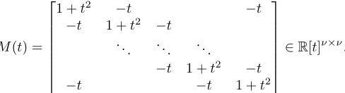
Definition 4.3. [36] Let A ∈ Rn×n be the adjacency matrix of an undirected
graph. For any t ∈ C, the associated deformed graph Laplacian is the Hermitian
matrix polynomial
M(t) =I−At+ (∆−I)t2∈R[t]n×n. (4.1)
Observe thatM(1) =Lis the graph Laplacian,M(0) =I is the identity matrix, whileM(−1) is the signless graph Laplacian [15].
Proposition 4.4 records some basic spectral properties of M(t) which were, in part, discussed also in [36].
Proposition 4.4. The following hold:
1. M(t) is a regular matrix polynomial, and0 is never an eigenvalue of M(t); 2. 1 is always an eigenvalue of M(t), with geometric multiplicity equal to the
number of connected components of the graph of A;
3. the geometric multiplicity of∞as an eigenvalue ofM(t)is equal to the num-ber of leaves, i.e., vertices of degree1, in the graph ofA(in particular, ∞is an eigenvalue ofM(t) if and only if the graph ofA has at least one leaf ); 4. −1 is an eigenvalue of M(t) if and only if the graph of A has at least one
bipartite component. In this case, the geometric multiplicity of−1is equal to the number of bipartite components of the graph of A.
Proof.
1. We have detM(0) = 1, and therefore det(M(t)) cannot be the zero polyno-mial; moreover, by the same argument, 0 is not an eigenvalue.
2. Observe that the graph Laplacian L is always a singular matrix, because A1= ∆1. Therefore, detM(1) = detL= 0. The nullity ofL, and hence the geometric multiplicity of 1 as an eigenvalue of M(t), is equal to the number of connected components in the graph ofA[35].
3. The geometric multiplicity of the infinite eigenvalue is the nullity of ∆−I, which is equal to the number of leaves in the graph ofA.
4. M(t) has the eigenvalue−1⇔the signless graph Laplacian is a singular ma-trix⇔the graph ofAhas at least one bipartite component [15, Proposition 2.1]; moreover the multiplicity of the eigenvalue 0 of the signless graph Lapla-cian, and hence the geometric multiplicity of−1 as an eigenvalue ofM(t), is equal to the number of bipartite components in the graph of A [15, Corollary 2.2].
In what follows, both in this section and in sections6and7, we will explore further the spectral properties ofM(t), obtaining several results that are, to our knowledge, new. The next proposition shows that, for disconnected graphs, it suffices to study the individual deformed graph Laplacians associated with each connected component. Proposition 4.5. Let A ∈ Rn×n be the adjacency matrix of a disconnected
M(t) be the deformed graph Laplacian associated with A and Mi(t)be the deformed graph Laplacians associated with Ai, for i= 1, . . . , c; and let λ∈C∪ {∞}. Then, λ
is an eigenvalue of M(t) if and only if it is an eigenvalue of Mi(t) for some value of i= 1, . . . , c. Moreover, denote by γ(λ)(resp. γi(λ)) the geometric multiplicity of
λ as an eigenvalue ofM(t) (resp. Mi(t)). Similarly, letα(λ) and αi(λ) denote the corresponding algebraic multiplicities. Then, it holds
γ(λ) = c
X
i=1
γi(λ), α(λ) = c
X
i=1
αi(λ).
Proof. Since the underlying graph is disconnected, by relabelling the nodes we see thatA(resp.,M(t)) is permutation similar to a block diagonal matrix (resp., matrix polynomial) whose diagonal blocks have sizes equal to the sizes of each connected component of the underlying graph. Clearly, each diagonal block Mi(t) is precisely the deformed graph Laplacian associated with the ith connected component. If λ∈
C, the statement is an immediate consequence of the observation above and of the definitions of multiplicities of an eigenvalue. If λ = ∞, the statement about the algebraic multiplicity requires a little extra care. To see it, note that denoting by ni the size of theith connected component of the graph
α(∞) = 2n−deg detM(t) = 2 c
X
i=1
ni
! −
c
X
i=1
deg detMi(t)
!
= c
X
i=1
αi(∞).
Proposition 4.4 does not say anything about the algebraic multiplicities of the special eigenvalues 1,−1,∞. We complete the picture with Proposition 4.6, which characterizes when these special eigenvalues are semisimple or defective in terms of features of the underlying graph.
Proposition 4.6.
1. The eigenvalue 1 of M(t)is semisimple if and only if there is no connected component of the graph of A having average degree precisely equal to 2; and it is simple if and only if the previous condition holds and the graph of A is connected.
2. Suppose that −1 is an eigenvalue ofM(t). Then, it is semisimple if and only if there is no bipartite connected component of the graph ofAhaving average degree precisely equal to2; and it is simple if and only if the previous condition holds and the graph ofA has only one bipartite connected component. 3. Suppose that∞is an eigenvalue ofM(t). Then, it is semisimple if and only if
every connected component of the graph of Awhich has a leaf is the complete graph with2 vertices. Moreover,∞ can never be a simple eigenvalue. Proof. By Proposition 4.5 we may assume without loss of generality that the graph ofA is connected.
Our proof is based on the following classical results in the theory of matrix polyno-mials [24]: a finite eigenvalueλof the matrix polynomialP(t) =Pki=1Atti, associated with the eigenvectorw, is defective if and only if there exists2a vectorvsuch that
P(λ)v+P′
(λ)w=0. (4.2)
2
Similarly, the eigenvalue∞, associated with the eigenvectorw, is defective if and only if there exists a vectorv such that
Akv+Ak−1w=0. (4.3)
Hence:
1. The eigenvalue 1 ofM(t) is associated with the eigenvector 1. Noting that M(1) =L and M′
(1) = 2L+A−2I, (4.2) becomes Lv+A1= 2·1. The latter equation has a solution if and only if (A−2I)1lies in the column space of L, or equivalently, 0 = 1T(A−2I)1= d−2n, where d = Pni=1degi is the sum of the degrees of all the nodes. Hence, 1 is defective if and only if d/n= 2, i.e., the average degree is 2.
2. The proof is analogous to the previous case, noting that if−1 is an eigenvalue of M(t) associated with a connected graph, then, since M(−1) =:Q is the signless graph Laplacian, the graph is bipartite and the associated eigenvector wis such thatwi=−wjfor every edgei↔j [15]. SinceM′
(−1) =A−2Q+ 2I, we see that−1 is defective if and only if 0 =wT(A+ 2I)w=−d+ 2n. 3. This time, we start from (4.3) and note that Ak = ∆−I and Ak−1 =−A.
Clearly, for every nodei which is a leafei is an eigenvector associated with
∞. Then, ∞is defective ⇔the equation (∆−I)v =Aei has a solution⇔
Aei is orthogonal toej for everyjwhich is in turn a leaf⇔the unique node connected to i is not itself a leaf. The only way for a connected graph to have two leaves connected to each other (and hence for∞to be a semisimple eigenvalue) is if the graph is the complete graph with two vertices. In this case, however,∞must have both algebraic and geometric multiplicity 2.
We now give a powerful auxiliary result.
Theorem 4.7. Let Abe the adjacency matrix of a simple, undirected, connected graph. Denote byAethe adjacency matrix, possibly of smaller size, such that the graph ofAeis obtained by removing from the graph ofAall the leaves, if any, and the edges connecting these leaves to the rest of the graph. Suppose that the graph of Ae is not empty, i.e., it contains at least one node. Let M(t), Mf(t) be the deformed graph Laplacians associated with A,Aerespectively.
Then, λ∈C is a finite eigenvalue ofM(t)if and only if it is a finite eigenvalue
of Mf(t). Moreover, the geometric multiplicities of λ as an eigenvalue of M(t) and f
M(t) are the same.
Proof. Suppose that there areℓleaves in the graph ofA. Ifℓ= 0, there is nothing to prove. Furthermore, the graph ofAeis not empty unlessℓ=n(andn= 2). Hence, we may assume 0< ℓ < n. Moreover, without loss of generality, we label the leaves in the graph ofAas nodes 1, . . . , ℓ.
Now, λ∈ C is a finite eigenvalue of M(t) if and only if there exists a nonzero v∈Cn such that
λ2(∆−I)v−Aλv+v=0. (4.4) Let degi denote the degree of node i. Clearly, degi = 1 fori≤ℓ, while fori > ℓwe set degi=ℓi+νi whereℓi is the number of leaves adjacent to nodei. Hence, (4.4) is equivalent to the following scalar equations: fori≤ℓ,vi=λvj, wherejis the unique node adjacent to nodei, while fori > ℓ
0 = (ℓi+νi−1)λ2vi+vi−λX j
vj= (ℓi+νi−1)λ2vi−λ2ℓivi+vi−λX k
where the first summation is over allj such that nodej is adjacent to nodei, while the second summation is over allk such that nodek is not a leaf and is adjacent to nodei. We rewrite the equations associated withi > ℓ as
(νi−1)λ2vi+vi−λX k
vk,
to see that a nonzero solution to (4.4) exists if and only if there is a nonzeroev∈Cn−ℓ such that
λ2(∆e −In−ℓ)ev−λAeve+ev=0,
where∆ = diag(diag(e Ae2)). To conclude the proof of the first statement, we note that
the latter holds if and only ifλis an eigenvalue of Mf(t).
By replicating the argument above γ times, we now build two sets ofγ nonzero vectors each, say,v(1),v(2), . . .v(γ)∈Cn, andve(1),ve(2), . . .ev(γ)∈Cn−ℓ, such that for
j= 1, . . . , γ,
M(λ)v(j)=0, Mf(λ)ve(j)=0, v(j)=
⋆
e
v(j)
,
where here and below⋆ denotes a block whose exact form is not relevant. The first set of vectors is linearly independent if and only if the second is. Indeed,
v(1) v(2) . . . v(γ)=
⋆ In−ℓ
e
v(1) ev(2) . . . ev(γ)
⇒rankv(1) v(2) . . . v(γ)= rankve(1) ev(2) . . . ve(γ)
This proves the statement on the the geometric multiplicities.
Theorem 4.7says that to compute the finite eigenvalues ofM(t) we are allowed to remove all the leaves of the underlying graph, and iterate the process until we are left with a graph with no leaves. (As a consequence, if the underlying graph is a forest, then the only finite eigenvalues are ±1, which must be both semisimple. This observation is recorded as Corollary7.1 in section 7, with an alternative proof based on the connection with NBTWs.) As we discuss in section8, the fact that the spectrum of the matrix polynomial does not “see” the leaves in a graph also has useful practical implications.
As our first application of Theorem4.7, we show that the deformed graph Lapla-cian can never have finite eigenvalues of modulus larger than 1.
Theorem 4.8. Let M(t) be the deformed graph Laplacian associated with a simple undirected graph. Suppose that λ ∈ C is a finite eigenvalue of M(t). Then,
|λ| ≤1.
Proof. By Proposition 4.5 and Theorem 4.7, we may assume with no loss of generality that the graph ofA is connected and that it does not have any leaves.
Ifλ∈Cis a finite eigenvalue of M(t), then there exists a nonzero v∈Cn such that (4.4) holds. Without loss of generality we takekvk2= 1. Premultiplying (4.4)
byv∗, we obtain
where α=v∗∆v
−1 and β =v∗Av. Denoting the degree of the ith node by deg
i, we have degi≥2 for alli, and henceα=P
n
i=1degi|vi|2−1≥2−1 = 1.
There are two cases. If λ6∈R, thenλ∗ is also an eigenvalue ofM(t) and a root of (4.5). It follows that 1≤α=|λ|−2 ⇔ |λ| ≤1. Suppose now λ∈R. Using also
the fact that ∆±A are both positive semidefinite matrices [15, 35], which implies
|β| ≤α+1, we have 0≤β2−4α≤(α−1)2, and hence,|λ| ≤(|β|+pβ2−4α)/(2α)≤
(α+ 1 +α−1)/(2α) = 1.
5. Nonbacktracking Walk Centrality and the Deformed Graph Lapla-cian. In section 3we gave a simple example where the NBTW centrality in Defini-tion 3.2could be computed from first principles. To obtain a general-purpose algo-rithm, we quote two results from the theory of zeta functions of graphs that concern the combinatorics of NBTWs. Although originally derived from a pure mathematics viewpoint, these results turn out to be extremely useful from the perspective of ma-trix computations in network science, and they also highlight a connection between NBTWs and the deformed graph Laplacian. Lemma 5.1 gives a recurrence relation between NBTW counts of different lengths. Theorem 5.2 is an immediate corollary that gives an expression for the associated generating function.
Lemma 5.1. [13, 43, 44] Recall that ∆ denotes the diagonal degree matrix and
pr(A) has (i, j) element that counts the number of NBTWs of length r from i to j. Then p1(A) =A,p2(A) =A2−∆, and forr >2
Apr−1(A) =pr(A) + (∆−I)pr−2(A). (5.1)
Theorem 5.2. [13,43,44] LetΦ(A, t) :=P∞r=0pr(A)tr, where, for convenience,
we set p0(A) =I, and recall thatM(t)denotes the deformed graph Laplacian associ-ated withA. Suppose moreover thatt is such that the power series converges. Then,
M(t)Φ(A, t) = (1−t2)I. (5.2)
In Definition3.2we see that the NBTW centralityxiof nodeimay be computed viax= Φ(A, t)1. From Theorem5.2we see that this simplifies to the linear system
M(t)x= (1−t2)1. (5.3) We note from (4.1) that, for any fixed value of t, M(t) in (5.3) has the same sparsity structure as the coefficient matrixI−αAthat appears in the original Katz system (2.2). Hence, NBTW centrality may be computed at the same cost as Katz centrality.
6. Further Spectral Analysis of the Deformed Graph Laplacian. Theo-rem6.1is an enhancement of Theorem4.7that relies on the results of Section5.
Theorem 6.1. Suppose, with the notation and assumptions of Theorem4.7, that
λ∈Cis a finite eigenvalue of bothM(t)andMf(t). Then, the algebraic multiplicities
of λas an eigenvalue ofM(t)andMf(t)are the same.
be node 2, and denote byAb(resp. Mc(t)) the adjacency matrix (resp. deformed graph Laplacian) of the graph obtained by removing node 1 and edge 1↔2. Manifestly,
1⊕Mc(t)=M(t)−
0 −t 0 . . .
−t t2 0 . . .
0 0 0 . . . .. . ... ... . ..
=M(t)−
0 −t
−t t2
0 0 .. . ...
1 0 0 . . . 0 1 0 . . .
.
By the matrix determinant lemma, and since det1⊕Mc(t)= detMc(t), we have
detMc(t) = detM(t) det
I2−
1 0 0 . . . 0 1 0 . . .
M(t)−1
0 −t
−t t2
0 0 .. . ... , and hence
detMc(t) detM(t)= det
I2−N(t)
0 −t
−t t2
,
having denoted by N(t) the top-left 2×2 block of M(t)−1. We now exploit
Theo-rem5.2and express [N(t)]22= (1 +f(t))/(1−t2), withf(t) :=P ∞
r=1artr, wherear
is the number of NBTWs of lengthrfrom node 2 to itself. Since node 1 is a leaf, and again by Theorem5.2, we observe that
[N(t)]11=
1 +t2f(t)
1−t2 , [N(t)]12=N(t)21=
t+tf(t) 1−t2 .
By direct computation, det
I−N(t)
0 −t
−t t2
= 1, so detMc(t) = detM(t).
We now work towards Theorem 6.3, which characterizes the graphs whose de-formed graph Laplacian has an eigenvalue of modulus<1. To this end, Lemma6.2
explicitly lists all the finite eigenvalues of the deformed graph Laplacian of a connected graph having average degree 2.
Lemma 6.2. Let A ∈ Rn×n be the adjacency matrix of a simple, undirected,
connected graph whose average degree is precisely 2, and let M(t) be the associated deformed graph Laplacian. Then, M(t) has precisely ν distinct finite eigenvalues, equal to the νth complex roots of unity: λk= exp (2kπi/ν), for 0≤k≤ν−1, where
3≤ν ≤nis the length of the unique cycle in the graph ofA. Moreover, the algebraic multiplicity ofλk is always2, whereas its geometric multiplicity is2 ifλk 6=±1 or it is1 otherwise.
2 1 3 6 8 9 7 4 5 11 10
Fig. 6.1.A connected graph with average degree2. This graph has11nodes,11edges, and one cycle of length4. A tree can be obtained by removing any one of the four edges of the unique cycle, i.e.,1 ↔2,2 ↔3, 3 ↔4 or4 ↔1. This graph is bipartite as the cycle has even length: if we replaced, for example,3↔4by4↔11, the unique cycle would have length5and the graph would no longer be bipartite.
In this case, as noted already in [36], the deformed graph Laplacian is (permuta-tion similar to) a circulant matrix polynomial of the form
M(t) =
1 +t2 −t −t
−t 1 +t2 −t
. .. . .. . ..
−t 1 +t2 −t
−t −t 1 +t2
∈R[t]ν×ν.
By standard results in the theory of circulant matrices (or by induction on ν), it is readily seen that detM(t) = (tν−1)2. This shows that theνth roots of unity are all
eigenvalues with algebraic multiplicity 2.
It remains to prove the statement on the geometric multiplicity. For the eigen-values 1 and (if ν is odd)−1, the statement follows by items 1-2 in Proposition4.6. Otherwise, letλ6=±1 satisfyλν = 1. Then the columns of the matrix
N(λ) =
λν−1 1
λν−2 λ
.. . ... λ λν−2
1 λν−1
are linearly independent. Indeed, the determinant of the 2×2 leading submatrix of N(λ) is λ−2(λ2−1) 6= 0. It is immediate to check that M(λ)N(λ) =0, which
concludes the proof.
Theorem 6.3. Let A ∈ Rn×n be the adjacency matrix of a simple undirected
graph, and let M(t) be the associated deformed graph Laplacian. Then, there exists a finite eigenvalueλ, with |λ|<1, of M(t) if and only if the graph of A has at least one connected component whose average degree is>2.
Proof. By Proposition 4.5, we can assume without loss of generality that the graph ofA is connected.
Suppose first that the average degree is<2. Then, the graph ofAis a tree, and the statement follows from Theorem4.7or, more directly, from Corollary7.1. Similarly, if the average degree is precisely 2, then the statement follows by Lemma6.2.
and f′(1)>0, implying by elementary analysis the existence of λ
∈(0,1) such that f(λ) = 0.
That f(0) = 1 and f(1) = 0 is an immediate consequence of M(0) = I and M(1) = ∆−A=:L. We haved=Pidegi>2n. Moreover,
f′(t) =∂detM(t)
∂t = trace(adjM(t)·M
′
(t)),
where adjX denotes the matrix adjugate of X. Evaluating att= 1,
f′(1) = trace(adjL·(2∆−A−2I)) =−2trace(adjL) + trace(adjL·A),
where for the last equality we exploited the relation adjL·L = 0. Let λ1 ≥ · · · ≥
λn−1 ≥ λn = 0 be the eigenvalues ofL and set p=Qn −1
i=1 λi. It is known [35] that
p >0 if the graph of Ais connected. It is straightforward to show that
adjL= p n11
T
implying trace(adjL) =pand trace(adjL·A) =pd/n. Hence,f′
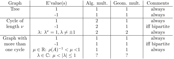
[image:14.612.77.439.433.556.2](1) =p(dn−2)>0. We now have a detailed picture of the finite spectrum of M(t) in terms of the features of the underlying graph. By Proposition4.5and Theorems4.7 and 6.1, we may focus on the case of a simple connected graph with no leaves. Table 6.1 then summarizes our results on the finite spectrum and includes an additional result that we state below as Proposition7.5.
Table 6.1
Spectra of the deformed graph LaplacianM(t)for various simple, undirected, connected graphs. Note that the condition of being bipartite is equivalent to not having any cycles of odd length. The symbol?refers to properties not studied in this paper.
Graph E’value(s) Alg. mult. Geom. mult. Comments
Tree 1 1 1 always
-1 1 1 always
Cycle of 1 2 1 always
lengthν -1 2 1 iff bipartite
λ: λν = 1, λ6=±1 2 2 always
Graph with 1 1 1 always
more than -1 1 1 iff bipartite
one cycle µ∈R: ρ(A)−1< µ <1 1 1 always λ∈C: µ <|λ| ≤1 ? ?
7. The Radius of Convergence of the Generating Function. The power series P∞r=0pr(A)tr makes sense mathematically for anyt ∈ C; although, as men-tioned in section 3, for network analysis it is natural to focus on t∈ (0,1)⊂R. In this subsection we study the radius of convergence of this power series to its gener-ating function (1−t2)M(t)−1. We note that it may happen that 1 or−1 are within
the radius of convergence but are also eigenvalues ofM(t), so that the latter is not invertible at t= 1 or t =−1. In this case, and with slight abuse of notation, when talking of (1−t2)M(t)−1 fort= 1 ort =
First, we note that, by construction, elementwise it holds that pk(A) =|pk(A)| ≤ |Ak|=Ak.
Hence,|t|< ρ(A)−1, whereρ(A) is the spectral radius ofA, surely suffices for
conver-gence, sinceP∞k=0Aktk has radius of convergenceρ(A) −1.
However, this condition is sufficient but not necessary, as shown by the star graph example of section3, where ρ(A) = √n−1 yet we have convergence for allt. More generally, if the graph A is a tree (or a forest) so that there are no cycles, then pk(A) = 0 for large enough values of k. It follows that Φ(A, t) is a polynomial in t, and the series converges for all t. This implies thatM(t) cannot have any finite eigenvalues other than±1; and both 1 and−1 must be eigenvalues by Proposition4.4
(and noting that any tree is bipartite). Since the average degree of any tree is<2, by Proposition4.6these eigenvalues are semisimple. This observation yields the following corollary on the spectral properties ofM(t) in the case of a forest.
Corollary 7.1. Suppose that A is the adjacency matrix of a forest, and let
M(t) be the associated deformed graph Laplacian. Then, M(t) has the only finite eigenvalues 1 and −1. Moreover, 1 and −1 are both semisimple eigenvalues. (By Proposition 4.2, these two properties are equivalent to ℓn(t) =t2−1, where ℓn(t) is the nth invariant polynomial ofM(t), as defined in Theorem 4.1.)
For a general A, our analysis is based on the properties of the deformed graph LaplacianM(t) as a matrix polynomial. The following technical lemma will be useful. It follows from the conditional converse to Abel’s Theorem on power series [16].
Lemma 7.2. For any z ∈C let P∞
k=0akzk be a power series with nonnegative real coefficients, i.e., ak ≥0 ∀ k∈N. Suppose that the power series converges to the
rational function p(z)/q(z), with p(z), q(z)∈ R[z] coprime polynomials, with radius
of convergence r >0. Then, q(r) = 0.
We are now ready to state our main result on the convergence of the matrix power seriesPrpr(A)tr. It turns out that it is determined by a particular eigenvalue ofM(t).
Theorem 7.3. Let Abe the adjacency matrix of a simple, undirected, graph. Let
M(t) =I−tA+t2(∆−I)be the associated deformed graph Laplacian, and let ℓn(t) be thenth invariant polynomial of M(t), as defined in Theorem 4.1.
The radius of convergence of the power series in Theorem5.2is equal to|χ|where
χ is the smallest (in modulus) zero of
r(t) := ℓn(t)
1−t2, (7.1)
whileχ:=∞if such a function does not vanish.
Moreover, letλbe the smallest (in modulus) eigenvalue of the matrix polynomial
M(t).
1. There exists µ∈(0,1]⊂R such that (i)µ=|λ| and (ii) µ is an eigenvalue
of M(t).
2. If µ <1, then|χ|=µ.
3. If µ= 1 is a semisimple eigenvalue of M(t), then the underlying graph is a forest andχ=∞.
4. If µ= 1is a defective eigenvalue of M(t), then|χ|=µ= 1.
Before proving Theorem7.3, we give a few remarks that should be kept in mind.
• By Proposition 4.6, if the underlying graph does not have any connected component with average degree 2, then 1 is a semisimple eigenvalue ofM(t), otherwise it is defective.
• By Proposition4.2, any zero ofr(t) is a finite eigenvalue ofM(t).
• Again by Proposition4.2, ifM(t) has at least one finite eigenvalue6=±1, or if at least one among 1 or−1 is a defective eigenvalue ofM(t), thenr(t) must have at least one zero.
• If−1 is an eigenvalue ofM(t), which happens for example if the graph ofA is bipartite, thenr(t) is actually a polynomial.
• The power series converges for anyt ∈Cif and only if r(t) does not vanish for anyt∈C, if and only ifℓn(t) = 1−t2.
Proof. [of Theorem 7.3] From Theorem 5.2, for any t ∈ C within the disk of convergence, the matrix power series converges to (1−t)2M(t)−1. Since M(t) is
polynomial, Φ(A, t) = (1−t2)M(t)−1 is a matrix rational function int(but generally
not another matrix polynomial). Observe that
M(t)−1= adjM(t)
detM(t),
where adjX denotes the matrix adjugate of X. The entries of adjM(t) are, up to a sign, the (n−1)×(n−1) minors of M(t). Let gn−1(t) be the monic GCD of the
entries of adjM(t), andgn(t) =κdetM(t) whereκ6= 0 is such that gn(t) is monic. Then, we see thatt0∈Cis a pole of (1−t2)M(t)−1 if and only if it is a zero of
gn(t) gn−1(t)(1−t2)
= ℓn(t) 1−t2,
where we used Theorem4.1. Hence, the radius of convergence must be equal to|χ|, whereχis the smallest (in modulus) zero of the rational functionr(t) in (7.1) if any, or χ =∞ if r(t) does not have any zero. We may now address the remaining four points in the theorem.
1. Note thatℓn(t)∈R[t] and that by constructionpk(A)≥0 elementwise. If the radius of convergence is ≤1, then the existence of a positive real eigenvalue µ such thatµ= |λ| follows by Proposition 4.2and by applying Lemma 7.2
elementwise. On the other hand, if the radius of convergence is >1, then clearly µ = 1, because 1 is an eigenvalue by Proposition 4.4 and because by Proposition 4.2 there cannot be roots of r(t) of modulus ≤ 1. Finally, µ=|λ|>0 follows by Proposition4.4.
2. Ifµ <1, thenr(µ) = 0 butr(t)6= 0 for|t|< µ, so it follows by the argument above thatχ=µ.
3. Suppose |χ| <1, then ℓn(χ) = 0, and hence detM(χ) = 0. Henceχ is an eigenvalue of M(t) of modulus strictly less than 1, thus contradicting µ =
|λ|= 1.Moreover, by Theorem4.8, if|χ| ≥1 then either|χ|= 1 orχ=∞. On the other hand, by Proposition4.6, since 1 is a semisimple eigenvalue there is no connected component of the underlying graph whose average degree is precisely 2; and by Theorem6.3we can exclude the possibility of a connected component with average degree>2, since otherwise we would haveµ=|λ|< 1. Hence, the graph is a forest and thereforeχ=∞by Corollary7.1. 4. If µ = 1 is a defective eigenvalue of M(t), then by Proposition 4.6 it is a
We note that, as a consequence of Theorem7.3 and the fact that |t| < ρ(A)−1
is a sufficient condition for convergence of the power seriesPkpk(A)tk, the following corollary gives a lower bound forµwhich is tighter than zero.
Corollary 7.4. Let M(t) be the deformed graph Laplacian associated with a graph with adjacency matrix Awhose spectral radius isρ(A). Then, every eigenvalue
λof M(t)satisfies|λ| ≥ρ(A)−1.
Theorem 7.3 reduces to the following simpler form assuming that µ <1, which by Theorem6.3is equivalent to assuming that the underlying graph has at least one connected component with average degree > 2. We note that this result therefore covers a general case that is likely to be encountered frequently in practice.
Proposition 7.5. Suppose that the matrix polynomialM(t) =I−tA+t2(∆−I) has an eigenvalueλwith|λ|<1. Then there exists a positive real numberµsuch that
µis the smallest (in modulus) eigenvalue ofM(t). Moreover, the radius of convergence of the power series P∞k=0tkpk(A)is equal to µ.
Furthermore, if the graph ofAis connected,µis a simple eigenvalue ofM(t)and every other finite eigenvalue λsatisfiesµ <|λ| ≤1.
Proof. Except for the last sentence, the statement is an immediate corollary of Theorem7.3.
To prove the last sentence, observe that by Theorem 6.3 the graph of A must have average degree>2, and hence, it must have at least two cycles. Moreover, by Theorem6.1we may assume that the graph ofAhas no leaves. Consider the directed graph obtained by replacing each undirected edge by two directed edges, with opposite orientations, between the same nodes; we label these directed edges 1, . . . ,2m. By Corollary 1 and equation (2.3) in [26],λ6=±1 is a finite eigenvalue ofM(t) if and only ifλ−16= 0,±1 is an eigenvalue of the 2m×2mmatrixB defined as follows: if there
exists a NBTW on the dircted graph that includes the consecutive directed edgesi and j then Bij = 1, otherwiseBij = 0. B is a nonnegative matrix. Suppose it is reducible, then there exist two directed edgesiandj such that there is no NBTW of the form· · ·i· · ·j· · ·. This contradicts the assumption that the original undirected graph is connected, without leaves, and with at least two cycles.
Hence,Bis nonnegative and irreducible, and the statement follows by the Perron-Frobenius theorem.
8. Practical Observations. In practice, given a specific, real network, we would like to know what range of choices are available for the parametert in (5.3). From Proposition7.5, in the generic case where there is at least one connected com-ponent with average degree > 2, the strict upper limit for t is given by λ, the smallest (in modulus) eigenvalue of M(t). From the theory of matrix polynomi-als [24, 32,34, 37, 38], one can show that thisλ may be equivalently defined as the reciprocal of the largest (in modulus) eigenvalue of the matrix
C:=
A I−∆
I 0
. (8.1)
For example, one could use the generalized Gershgorin theorem [5, Theorem 3.1], obtaining that, if degj is the jth diagonal element of the matrix ∆, then no finite eigenvalue ofM(t) can possibly lie in the region
n
\
j=1
{λ∈C:|1 + (deg
j−1)λ2|>degj|λ|},
which, denoting by degmaxthe maximum degree of the graph ofA, for|λ|<1 can be shown to reduce to{|1 + (degmax−1)λ2|>degmax|λ|}.
Alternatively, bounds specific for matrix polynomials based on tropical algebra exist [6,39]. For example, by [39, Theorem 3.1, item(ii)] ifk · kis any induced matrix norm then |λ| ≥ r where r is the unique positive root of the quadratic polynomial x2k∆−Ik+xkAk −1. Solving the quadratic equation gives
|λ| ≥ p
kAk2+ 4k∆−Ik − kAk
2k∆−Ik .
Now, kAk2 =ρ(A) while kAk1 =kAk∞ = degmax, whereas (assuming that the
graph ofAhas at least one edge, so that ∆6= 0)k∆−Ik= degmax−1 for all the three
norms considered above. Since ρ(A)<degmax, the spectral norm gives the strongest
of the three bounds:
|λ| ≥ p
ρ(A)2+ 4 deg
max−4−ρ(A)
2 degmax−2
and we deduce that a sufficient condition for convergence is
0< t <
p
ρ(A)2+ 4 deg
max−4−ρ(A)
2 degmax−2
.
Theorem 4.7 shows that the spectrum of M(t) does not change when a leaf is removed from the graph. It follows that, as a practical approach, we can preprocess the graph by iteratively removing all leaves. Suppose this gives a matrixAbof dimension
b
n×bn. Then the techniques in this section for computing or bounding the radius of convergence may be applied to A, rather thanb A, leading to a gain in efficiency when nb ≪ n, that is, when there are many, or large, trees dangling off the graph. Furthermore, the linear system (5.3) for NBTW centrality may be solved withA. Theb centralityxL for any node L that was removed as a leaf is then recoverable via the iterative relationxL= 1 +t(xN−t). Here,xN denotes the centrality of the node that was the neighbour of nodeL at the stage where nodeLwas removed3.
We also mention that recursive leaf removal corresponds to finding the 2-core of a graph. It is interesting to note that computingk-cores, and correspondingk-shells, has itself been proposed as a way to identify influential spreaders in a network [29]; although recent work has pointed out limitations of this approach [41].
9. Connection with M-matrix Theory. Suppose that 0 ≤t < min{1,|χ|}
where χ is defined as in Theorem 7.3. Theorem 7.3 implies that the power series
3
P
rpr(A)tr converges to (1−t2)M(t)
−1, and as a consequenceM(t)−1≥0
elemen-twise. In this section, we give a more direct proof of this fact using the theory of M-matrices. The proof relies on the observation that M(t) is a Hermitian matrix polynomial, and employs arguments that are typical in the theory of Hermitian ma-trix polynomials [34].
By Theorem 7.3, the two conditions t < |χ| and t < 1 imply that t is strictly smaller than the smallest real positive eigenvalue ofM(t). Now, letM be the matrix obtained by evaluatingM(t) att=t0for some 0≤t0<|χ|. Note thatM(0) =Ihas
npositive eigenvalues. Since the eigenvalues of a matrix depending continuously on a parametert are continuous as a set (see [27, Ch. II], [34, Sec. 5] for more details), and sinceM(t) is symmetric and not singular for allt∈[0, µ), necessarilyM =M(t0)
has all positive eigenvalues as well.
Now, note that M is a Z-matrix [40], i.e., its off-diagonal elements are≤0. By [40, Theorem 1], a Z-matrix such that all its eigenvalues have positive real part is an M-matrix. Hence, M is an M-matrix. As a consequence, again by [40, Theorem 1], M−1is a nonnegative matrix.
10. Limiting Behavior of the NBTW centrality Measure. In [4, Theorem 5.1], Benzi and Klymko study the limiting behaviour of classical parameter-dependent centrality measures for undirected networks, letting the parameter tend to the end-points of the convergence interval. In this section we study the limiting behaviour of the NBTW centrality measure.
Theorem 10.1. Let A be the adjacency matrix of a simple, connected, undi-rected graph, letM(t)be the associated deformed graph Laplacian, and let x(t)be the vector of the corresponding NBTW centrality measure defined as in Definition3.2 or equivalently in (5.3), witht∈(0,|χ|) andχdefined as in Theorem 7.3.
1. As t→0+, the rankings produced byx(t) converge to those produced by the vector of the degree centralities.
2. Suppose further that|χ| ≤1, so that by Theorem7.3we have0<|χ|=µ≤1, where µ is the smallest positive eigenvalue of M(t). Then as t → |χ|−
the rankings produced byx(t)converge to those produced by the eigenvector vof the matrix polynomial M(t)associated with the eigenvalue µ.
Proof. Part 1 may be proved by essentially the same argument given in [4, Proof of Theorem 5.1, item (i)], except that one has to replace [f(tA)1]iby [(1−t2)M(t)−11]i.
Indeed, expanding in powers oft,
[(1−t2)M(t)−11]i= [I1+At1+p
2(A)t21+. . .]i,
which for t →0+ behaves as 1 + deg
it+O(t2), where degi is the degree of theith node of the graph ofA. Hence, the statement follows.
For part 2, observe first that µhas geometric multiplicity 1 as an eigenvalue of M(t). This follows from Proposition 7.5ifµ <1 and from Proposition4.4 ifµ= 1. Note that, for any fixedt < µ,M(t) is a symmetric matrix which can be orthogonally diagonalized, say,M(t) =Q(t)Λ(t)Q(t)T, and hence
x(t) = (1−t2)Q(t)Λ(t)−1Q(t)T1. (10.1) Moreover, Q(t) and Λ(t) can be taken to be real-analytic functions of t [27, 34]. Now, let v be the eigenvector of the matrix polynomial M(t) associated with the eigenvalueµ, andkvk2 = 1 . Then, the matrixM(µ) has a simple eigenvalue 0 and
any fixed 0< t < µ, where the labelling is such thatλ1(µ)≥λ2(µ)≥ · · · ≥ λn(µ).
Letting qi(t) be the corresponding normalized eigenvectors, we can expand (10.1) as x(t) = (1−t2)q
n(t)T1λ−n1(t)qn(t) +O(λn(t)/λn−1(t)). Now, observing that4
ˆ
x(t) = λn(t) (1−t2)qT
n(t)1 x(t)
gives the same rankings as x(t) for any 0 < t < µ, since the two vectors are pro-portional. Noting that qn(t)→v and λn(t)/λn−1(t)→0 ast →µ−, we have that
ˆ
x(t)→v fort→µ−
, yielding the statement.
Theorem 10.1 has the following, somewhat surprising, consequence: a Perron-Frobenius-like result for the deformed graph Laplacian.
Theorem 10.2. LetAbe the adjacency matrix of a simple, connected, undirected graph and M(t) be the corresponding deformed graph Laplacian. Let µ ≤ 1 be the smallest real positive eigenvalue µ of M(t). Then, the corresponding eigenvector v
can be chosen to be componentwise nonnegative.
Equivalently, under the same assumptions, the eigenvector associated with the dominant eigenvalueµ−1 of the matrixCin (8.1) can be chosen to be componentwise nonnegative.
Proof. The first part of the statement is an immediate consequence of Theo-rem 10.1. The second part follows from the first part and the theory of companion linearizations of monic matrix polynomials, see for example [24,32,37,38].
Note that, by [33, Equation (17)], the limiting behaviour of the NBTW centrality measure characterized in Theorems 10.1and 10.2corresponds precisely to the non-backtracking eigenvector centrality introduced in [33]. It is worth emphasizing that this is generally different from the classical eigenvector centrality, thus showing that (unlike classical centrality measures) our newly proposed centrality measure doesnot
follow the “universal” limiting behaviour for largetdescribed in [4, Theorem 5.1]. At this stage it is useful to return to the star example (3.1). We know from the first principles derivation in section 3, or from Corollary 7.1 and Theorem7.3, that the radius of convergence for the generating function is infinite. In this case the nonbacktracking eigenvector centrality in [33], which can be computed via “the leading eigenvector” of the matrix C in (8.1), corresponds to the limit t→ 1. This measure has the attraction of being parameter free. However, in this example there are two dominant eigenvalues at ±1. In order to obtain nonnegative entries in the corresponding eigenvector, we must choose the eigenvalue +1. The associated eigen-vector corresponds to the null space of the graph Laplacian, and hence it is the eigen-vector of all ones. So, nonbacktracking eigenvector centrality assigns the same value to all nodes in the star. We regard this as unsatisfactory behavior, caused by the aim of completely eliminating the localization effect. Indeed, ranking the center of a star above its neighbors has been suggested as a basic “axiom” for centrality measures, [7,22].
The more general NBTW centrality measure introduced in this work may then be regarded as a means to interpolate between this extreme case and the opposite extreme of degree centrality.
4
Note that here we requireqT
n(t)16= 0. This is true because, by our previous analysis, evaluating M−1
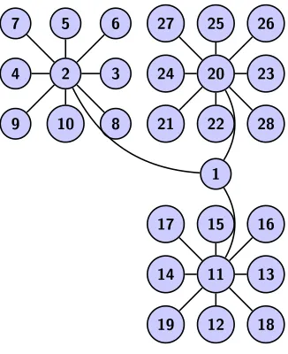
11. Synthetic Example: Galaxy Network. We now present a class of large scale networks where constraining to NBTWs can be shown to give qualitatively different, and potentially beneficial, results. We consider the case wheremcopies of the star graph with adjacency matrix (3.1) are joined together via a single central node which is linked to the central node of each star. Figure11.1illustrates the case wherem= 3 and n= 9. We will refer to such a structure as agalaxy graph.
2
10 3 4
5 6
7
8 9
24 20
25
22 23 26 27
28 21
1
15
11
12 13 14
16 17
[image:21.612.176.339.176.376.2]18 19
Fig. 11.1. A galaxy graph with m = 3stars, each with n= 9 vertices. Having labelled the vertices as within the figure, for this galaxy graph we say that the vertex 1 is galaxy-central, the vertices2,11,20are star-central, and every other vertex is peripheral.
We wish to analyze the walk-based centralities in detail. In each case, by sym-metry, there are at most three distinct values for the entries of the centrality vector x, corresponding to the three types of node. Along with x1, we will take x2 as a
representative of the star-central nodes (with indices xkn+2 fork = 0,1, . . . , m−1)
andx3 as a representative for the remaining peripheral nodes.
For degree centrality (which is also the α →0+ and t → 0+ limit of the other
centralities considered) we clearly have x1 = m, x2 = n and x3 = 1. Hence, for
m > n, the galaxy-central node ranks highest. In the case m ≤ n, there is still a case to be made for node 1 to be the most central—intuitively it is best positioned to initiate traversals around the network. We show below that even withm=O(1) as n→ ∞, it is possible for NBTW centrality to rank the galaxy-central node highest, whereas Katz and eigenvalue centrality always placex2> x1.
Still labelling by A the adjacency matrix of the star graph, and letting e1 =
1 0 . . . 0T ∈Rn, the galaxy graph has adjacency matrix
B =
0 eT1 . . . eT1 e1 A
..
. . ..
e1 A
.
For Katz centrality, it is useful to know the eigenvalues of B. Definea± = (n−
1)−1/4
Qbe any orthogonal matrix whose first two columns area+/|a+|and a−/|a−|, then
QTAQ=D:= diag(√n−1,−√n−1,0, . . . ,0). Moreover, byQ(e
1−e2) = √
2e1we
deduce thatQTe
1= 2−1/2(e1−e2) =:vand henceB is similar to
0 vT . . . vT
v D
..
. . ..
v D
,
which in turn is permutation similar to (denoting by1∈Rmthe vector of all ones)
0m(n−2)⊕
0
1T/√2 −1T/√2 1/√2 √n−1·Im 0
−1/√2 0 −√n−1·Im
.
Computing the characteristic polynomial of the (2m+ 1)×(2m+ 1) matrix above is immediate. For example, Schur complementing we get
λ2−(n−1)m
λ−m2 λ2−2λ(n−1)
=λ λ2−(n−1)m−1 λ2−(m+n−1).
We conclude that the Katz measure requires 0< α <(m+n−1)−1/2.
The Katz system, (I−αB)x=1, solves directly to give x1=
1 + (m−1)(n−1)α2+mα
1−(m+n−1)α2 , x2=
1 +nα
1−(m+n−1)α2, (11.1)
and
x3=
1 +α+α2(1−m)
1−(m+n−1)α2.
For NBTW centrality, we may work from first principles.
• The galaxy-central node 1 has mNBTWs of length one, m(n−1) NBTWs of length two, and no NBTW of length≥3.
• From each star-central node, such as node 2, there aren NBTWs of length one,m−1 NBTWs of length two, (m−1)(n−1) NBTWs of length three, and no NBTW of length≥4.
• From each peripheral node, such as node 3, begin one NBTW of length one, n−1 NBTWs of length two,m−1 NBTWs of length three, (m−1)(n−1) NBTWs of length four, and no NBTWs of length≥5.
Hence, we have
x1= 1 +mt+m(n−1)t2, x2= 1 +nt+ (m−1)t2+ (m−1)(n−1)t3, (11.2)
and
x3= 1 +t+ (n−1)t2+ (m−1)t3+ (m−1)(n−1)t4. (11.3)
Whetherx1> x2depends, for either centrality index, not only on the parameters,
αort, but also on mandn.
For both Katz and NBTW centrality, imposing x1 > x2 yields that α (resp. t)
centrality measures givex1> x2 for all valid parameter values—the degree centrality
ranking prevails. However, ifn > m, it could happen that 1/ρ(B) is smaller than this critical value, and hence Katz fails to have a transition tox2> x1when NBTW does.
Katz fails to have such a transition when
(n−m)2(m+n−1)>(n−1)2(m−1)2 (11.4)
and one way to achieve this whenn→ ∞is ifm=O(nγ) withγ≤1/2.
For example, let us analyze what happens ifm=O(1) while lettingngrow. We see in (11.1) that Katz always givesx2> x1in this regime, but for the NBTW version
in (11.2), the choice of t is crucial. To be concrete, fixing m = 5 we find that the inequality (11.4) is satisfied forn >21. Recall thatα <1/√n+ 4 in this setting. We obtain for the Katz centrality
x1
x2
=1 + 4(n−1)α
2+ 5α
1 +nα ,
which implies that x1/x2 =O(1/√n) whenn grows andαis a given fraction of its
upper bound. Conversely, for the NBTW centrality
x1
x2 =
1 + 5t+ 5(n−1)t2
1 +nt+ 4t2+ 4(n−1)t3.
Here,x1 > x2 for t >(n−5)(4n−4) ≈O(1/4), and, for example, setting t = 1/2
yieldsx1/x2≈5/4 for largen.
For further comparison, we note that since we know that the largest eigenvalue ofB is√m+n−1, and again using the symmetry, it is straightforward to compute the Perron-Frobenius eigenvector ofB, and hence, the eigenvector centrality for the galaxy graph. We find that
x1
x3
=m, x2 x3
=√m+n−1 =⇒ xx1 2
= √ m
m+n−1.
Again, we note that forn > m2 this yieldsx 2> x1.
In summary, in this example restricting to nonbacktacking walks can produce dramatically different results, and can highlight the galaxy-central node even when its degree is arbitrarily smaller than that of the star-central nodes.
We also recall the behavior of nonbacktracking eigenvector centrality on a star graph, as discussed at the end of section 10. The same effect arises here: taking the t → 1−
limit in (11.2) and (11.3), we see that all nodes are assigned the same centrality value by this measure.
12. Tests on Real Data.
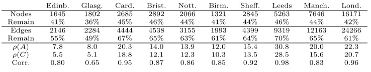
Table 12.1
Twitter networks for ten UK cities. First and second row: original number of nodes and percentage of nodes that remain after pruning. Third and fourth row: same information for edges. Fifth and sixth row: spectral radius ρ(A) relevant for Katz andρ(C)relevant for NBTW. Seventh row: Kendall’sτcorrelation between Katz and NBTW centrality for the top 100 Katz-ranked nodes.
Edinb. Glasg. Card. Brist. Nott. Birm. Sheff. Leeds Manch. Lond.
Nodes 1645 1802 2685 2892 2066 1321 2845 5263 7646 16171
Remain 41% 36% 45% 46% 44% 41% 44% 46% 44% 42%
Edges 2146 2284 4444 4538 3155 1993 4399 9319 12163 24266
Remain 55% 49% 67% 65% 63% 61% 64% 70% 65% 61%
ρ(A) 7.8 8.0 20.3 14.0 13.9 12.0 15.4 30.8 20.0 22.3
ρ(C) 5.5 5.1 18.8 12.1 12.3 10.3 13.5 28.5 15.6 20.7
Corr. 0.80 0.65 0.95 0.87 0.86 0.85 0.92 0.98 0.83 0.96
(fourteen nodes) and 1 (twenty-one nodes). The adjacency matrix A and the two-by-two block matrix C in (8.1) have spectral radius ρ(A) = 4.26 and ρ(C) = 1.39. For the Katz and NBTW centrality measures, we used 90% of the upper limit; that is, α= 0.9/ρ(A) = 0.21 for Katz and t = 0.9/ρ(C) = 0.65 for NBTW. Figure12.1
displays the network twice, with the size of each node proportional to the centrality, using Katz on the left and NBTW on the right. We see that the NBTW version is less closely tied to the nodal degree, and in particular does not emphasize the high degree node to the same extent. The lower picture in Figure12.1scatter plots the two centrality measures, normalized to have maximum component equal to one. This further clarifies that NBTW centrality has delocalized the high degree node, and also shows that the two measures give different rankings, even at the high end— the top 10 nodes, in descending order, are 1,2,13,4,8,7,21,3,12,6 for Katz and 1,2,7,13,21,17,36,4,8,3 for NBTW.
Looking at the localization effect in larger networks, withn= 50,000 we called
pref(n,2)and added an extra 100 undirected edges uniformly at random, deleting repeated edges. Using 500 independent preferential attachment network samples of this type, the average inverse participation ratio (3.8) for degree centrality was found to be 0.06, and for Katz with α= 0.9/ρ(A) it was the same order of magnitude at 0.05. For NBTW centrality witht = 0.9/ρ(C), this value decreased by an order of magnitude to 0.003. (In all cases the standard error was below the precision displayed.) 12.2. Pruning. Next, we illustrate the effect of iteratively pruning the leaves from a network, as discussed in section 8. On the left in Figure 12.2 we show the largest connected component of a protein-protein interaction network for yeast [46]. There are 564 nodes and 687 edges. After removing leaves until none remain, we arrive at the network on the right, with 167 nodes and 290 edges. Using larger protein-protein interaction networks from the Integrated Interactions Database [30] (downloaded on 13th of June, 2016), we found that leaf pruning reduced the number of nodes and edges, respectively, as follows; worm: 4853 7→ 2628, 12635 7→ 10480; fly: 91397→7303, 499597→48146; mouse: 75697→4583, 192687→16346. Similarly, Table12.1summarizes results for reciprocated mention Twitter networks in ten UK cities, taken from [25]. We see that more than half of the nodes and typically around a third of the edges are eliminated. We conclude that pruning to reduce problem size is a viable option for some real problem classes.
Fig. 12.1. Centrality measures for a preferential attachment network. Upper pictures have node size proportional to Katz (left) and NBTW (right) centrality. Lower picture scatter plots the two centrality measures.
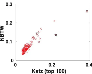
for NBTW. We then found the top 100 nodes according to the Katz measure, and for these nodes, computed the correlation between the two centrality measures. Following the recommendations in [42], we quantify correlation with Kendall’sτ coefficient. The spectral radii are seen to be close and the correlations high, with the noteworthy exception of Glasgow.


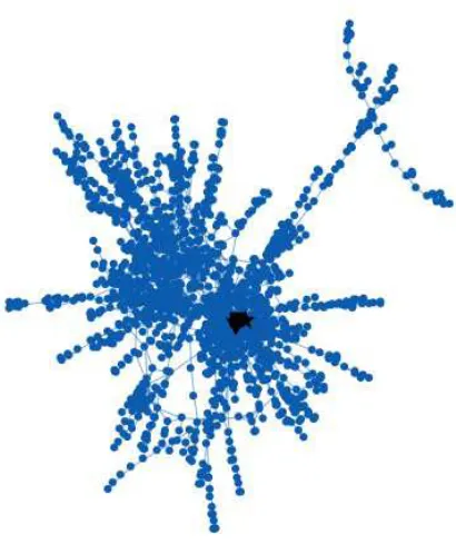

![Fig. 12.6.The yeast protein interaction network from [17, 18, 21]. Essential nodes are markedwith a darker symbol](https://thumb-us.123doks.com/thumbv2/123dok_us/1383409.91524/30.612.175.376.240.480/yeast-protein-interaction-network-essential-markedwith-darker-symbol.webp)
