© Research India Publications http://www.ripublication.com
Tuning of FOPID Controller for Meliorating the
Performance of the
Heating Furnace Using
Conventional Tuning and Optimization Technique
Amlan Basu1, Sumit Mohanty2 and Rohit Sharma3
1,3Research Scholar (M.Tech.), Department of Electronics and Communication
Engineering, ITM University, Gwalior, Madhya Pradesh – 475001, India
2Assistant Professor, Department of Electronics and Communication Engineering,
ITM University, Gwalior, Madhya Pradesh – 475001, India
Abstract
The milieu of the paper is the melioration of the performance of heating furnace, which is done by the tuning of the fractional order proportional integral derivative (FOPID) controller using various tuning techniques and the optimization algorithms. These techniques help us to find out the standards of the integer order tuning parameters and also the fractional order parameters of the PID controller. The Astrom-Hagglund and the Chien-Hrones-Reswick methods of tuning are used for tuning the tuning parameters of the controller, where Nelder-Mead optimization technique is used for optimizing the values of differ-integrals. These standards of parameters obtained using mentioned tuning techniques help us to generate standardized differ-integral order of the FOPID controller. This helps to improve the performance of the heating furnace. The complete process has been executed after the approximate dynamic modelling of the heating furnace.
1. INTRODUCTION
Models portray our convictions about how the world functions. In mathematical modeling we make an interpretation of those convictions into the dialect of mathematics [1]. This has numerous focal points, (i) Mathematics is an extremely exact dialect. This helps us to formulate thoughts and distinguish fundamental suppositions, (ii) Mathematics is a succinct dialect, with very much characterized rules for controls, (iii) every outcome that mathematicians have demonstrated over many years are available to us and (iv) computers can be utilized for performing the numerical computation [1] .
There is an expensive component of trade off in mathematical modeling. The dominant part of interacting systems in this present reality is very muddled to model completely. Subsequently the first level of trade off is to distinguish the most critical parts of the framework. These will be incorporated into the model, the rest will be avoided. The second level of the trade off concerns the measure of mathematical manipulation which is beneficial. Despite the fact that the mathematics can possibly demonstrate the general results, these outcomes depend fundamentally on the type of comparisons utilized. Little changes in the structure of comparisons may require colossal changes in the mathematical methods. Utilizing computers to handle the model mathematical equations might never prompt exquisite results, however it is very much stout against modification [2].
A heating furnace is basically a thermal fenced in area and is utilized to process the unprocessed (raw) substances at high temperature both in fluid and solid state. A few commercial enterprises like iron and steel making non-ferrous metals creation, glass making, assembling, earthenware handling, calcination in generation of cement, et cetera utilize the heating furnace. The principle goals are, (a) to use the heat effectively with the goal that misfortunes are least and (b) to handle the distinctive stages (solid, fluid and gas) moving at diverse velocities for diverse time and temperatures such that wearing away and deterioration of the obstinate are least
The principle components of the heating furnace are the energy sources (fossil fuel, electric energy, and chemical energy), appropriate refractory material, exchanger of heat and the control and instrumentation. Heaters are utilized for wide assortment of handling of raw substances to completed items in a few commercial enterprises. Comprehensively they are utilized either for physical preparing or for concoction handling of raw substances. In the physical handling the condition of the reactants stays unaltered; though in the compound preparing condition of the reactants changes either to fluid of gas [3].
Now coming to the proportion integral derivative (PID) controller then it will be engrossing to note that ninety percent of the cutting edge controllers being utilized today are the proportion integral derivative (PID) controllers or the revised proportional integral derivative (PID) controller [4].
stayed critical in the perspective of its execution [5]. Since a large portion of the proportion integral derivative (PID) controllers are adjusted in adjacent, an extensive variety of sorts of tuning standards have been proposed in the writing. Using the tuning gauges, delicate and aligning of proportional integral derivative (PID) controllers can be made adjacent. In like manner, modified tuning methods have been made and a rate of the proportional integral derivative (PID) controller may have online customized tuning limits. Balanced sorts of proportional integral derivative (PID) control, for instance, I-PD control and multi degrees of flexible Proportional integral derivative (PID) control are at this time being utilized as a part of industry. Various sober minded frameworks for knock less changing (from manual operation to customized operation) and build booking are financially open. The handiness of proportional integral derivative (PID) controls laid in their general relevance to most control systems. In particular, when the exploratory model of the plant is not known and thus investigative layout techniques can't be used, proportional integral derivative (PID) controls winds up being generally supportive. In the field of procedural control systems, it is unquestionably comprehended that the central and the amended proportional integral derivative (PID) control techniques have shown their accommodation in giving attractive control, regardless of the way that in various given circumstances they may not give wonderful control.
The FOPID controller which has been developed from the Proportional integral derivative (PID) controller by just renovating it into fractional order from the integer order which was first proposed in 1997 by Igor Podlubny [6]. In addition, the enticement behind the utilization of FOPID is that it is very trouble-free to design the controller for systems with higher order by using the practices of modeling based on regression and also because it has the iso-damping property which makes possible the variation over ample range of operating point for a particular controller [7]. There are numerous other motives which are accountable for the utilization of FOPID controller and they are the burliness from the high frequency noise as well as for the gain variation of the plant, the nonexistence of the steady state error and it holds both the phase and gain margin and also the gain and phase cross over frequency [8].
Optimization also termed as augmentation is the procedure of creating the things more unblemished, potent and dynamic in order to acquiesce the best result. The various techniques of optimization are Nelder-Mead, Active-Set, Interior-Point, SQP (sequential quadratic programming) et cetera. Numerically it can be explained as the procedure of expanding and shrinking of the endeavor capacity relying upon various conclusion variables under a deal of restrictions. The optimization technique has been used so as to discover and attain the finest results so as to design the most accurate FOPID controller that yields the finest output and assists the plant to augment its performance.
2. PID CONTROLLER
PID stands for the proportional integral derivative which can be defined numerically using differential equation as,
𝑢(𝑡) = 𝐾𝑝𝑒(𝑡) + 𝐾𝑖∫ 𝑒(𝜏)𝑑𝜏0𝑡 + 𝐾𝑑𝑑𝑒𝑑𝑡 (1)
On performing the Laplace transform of the equation (1) which is the PID controller equation is,
𝐿(𝑠) = 𝐾𝑝+ 𝐾𝑠𝑖+ 𝐾𝑑𝑠 (2)
Where, Kp is the gain of proportionality, Ki is the gain of Integral, Kd is the gain of
Derivative, e is the Error (SP-PV), t is the instantaneous time and τ is the variable of integration that takes on the values from time 0 to the present t.
3. FOPID CONTROLLER
The FOPID controller can be defined numerically using differential equation as [6], 𝑢(𝑡) = 𝐾𝑃 𝑒(𝑡) + 𝐾𝑖𝐷𝑡−𝜆𝑒(𝑡) + 𝐾
𝑑𝐷𝑡𝜇𝑒(𝑡) (3)
FOPID stands for the fractional order proportional integral derivative. The equation of the FOPID in Laplace domain is [5],
𝐿(𝑠) = 𝐾𝑝+ 𝐾𝑖
𝑠𝜆+ 𝐾𝑑𝑠𝜇 (4) Where, Kp is the gain of proportionality, Ki is the gain of Integral, Kd is the gain of
Derivative and λ and μ are the differential-integral’s order for FOPID controller.
4. A PRÉCIS ON FRACTIONAL ORDER CALCULUS
Fractional order calculus is a mathematical concept that has been in existence from 300 years ago [9]. It is the mathematical concept that has proved itself better as compared to the integer order methods.
According to Lacroix,
𝑑𝑛 𝑑𝑥𝑛𝑥𝑚 =
𝑚!
(𝑚−𝑛)!(𝑥)(𝑚−𝑛)=
Г(m+1)
Г(𝑚−𝑛+1) (𝑥)(𝑚−𝑛) (5)
According to Liouville, 𝐷−12𝑓 = 𝑑
−1 2𝑓
(𝑑(𝑥−𝑎))−12 = 1
Г(12)∫ (𝑥 − 𝑢)
−1 2
𝑢=𝑥
𝑢=𝑎 𝑓(𝑢)𝑑𝑢 = 𝐹
−1
According to Riemann-Liouville [10],
a𝐷𝑡𝛼𝑓(𝑡) =
1 Г(𝑚−𝛼)(
𝑑 𝑑𝑡)
𝑚∫ 𝑓(𝜏)
(𝑡−𝜏)1−(𝑚−𝑎)𝑑𝑡
𝑡
𝑎 (7)
According to Grunwald-Letnikov, which is being used widely is,
a𝐷𝑡𝛼𝑓(𝑡) = 𝑙𝑖𝑚
1
⎾(𝛼)ℎ𝛼∑ {
⎾(𝛼+𝑘)
⎾(𝑘+1)}𝑓(𝑡 − 𝑘ℎ)
(𝑡−𝑎) ℎ
𝑘=0 (8)
Where,
Г(𝑡) = ∫ 𝑥∞ 𝑡−1𝑒−𝑥𝑑𝑥
0 (9)
This is called the Euler’s gamma function.
The fractional order derivatives and integrals properties are as follows [11],
f(t) being a logical function of t then the fractional derivative of f(t) which is
0𝐷𝑡𝛼𝑓(𝑡) is an analytical function of z and α.
If α = n (n is any integer) then 0𝐷𝑡𝛼𝑓(𝑡) produces the similar result as that of the
traditional differentiation having order of n.
If α=0 then 0𝐷𝑡𝛼𝑓(𝑡) is an identity operator 0𝐷𝑡𝛼𝑓(𝑡) = 𝑓(𝑡) (10) The differentiation and integration of fractional order are said to be linear
operations,
0𝐷𝑡𝛼𝑓(𝑡) + 𝑏𝑔(𝑡) = 𝑎0𝐷𝑡𝛼𝑓(𝑡)𝑏0𝐷𝑡𝛼𝑓(𝑡) (11) The semi group property or the additive index law,
0𝐷𝑡𝛼𝑓(𝑡)0𝐷𝑡𝛽𝑓(𝑡)=0𝐷𝑡𝛽𝑓(𝑡)0𝐷𝑡𝛼𝑓(𝑡)=0𝐷𝑡𝛼+𝛽𝑓(𝑡) (12)
Which is being held under some sensible limitations on f(t).Derivatives which are of fractional order has the commutation with derivative of integer order which is as follows,
𝑑 𝑛
𝑑𝑡𝑛a𝐷𝑡𝛼𝑓(𝑡) =a𝐷𝑡𝑟(
𝑑𝑛𝑓(𝑡)
𝑑𝑡𝑛 ) =a𝐷𝑡𝑟+𝑛𝑓(𝑡) (13)
where for t=a, f(k)(a)=0 for k={0,1,…n-1}.The given equation shows that 𝑑𝑛
5. DYNAMIC MODELING OF HEATING FURNACE
The approximate modeling of heating furnace includes quantity of input that varies with time and is actually the fuel mass gas flow rate and also the pressure inside the furnace which is the output value.
The dynamic modeling of heating furnace includes the mass, energy and the momentum balances. It also includes the transfer of heat from the hot flue hot gas to water, flue gas flow from the boiler model and steam model.
As we know for any physical system the total force is equal to the summation of individual forces exerted by mass (m), damping (b) and spring (k) element [12]. Mathematically we can state the same as,
𝐹 = 𝑚𝑎 + 𝑏𝑣 + 𝑘𝑥 (14)
In the equation (14) acceleration is signified as a, velocity is signified as v and displacement is signified as x.
Therefore the differential equation of equation (14) is,
𝐹 = 𝑚𝑑𝑑𝑡2𝑥2+ 𝑏𝑑𝑥𝑑𝑡+ 𝑘𝑥 (15)
Note: For designing a network based PID the above equation or model is a rough process behavior description.
Therefore, the differential equation of the heating furnace using the above equation becomes [13],
𝐹 = 73043𝑑𝑑𝑡2𝑥2 + 4893𝑑𝑥𝑑𝑡+ 1.93𝑥 (16)
The Laplace transfer function of equation (16) which gives the Integer order model (IOM) as [14],
GI(s) =
1
73043𝑠2+4893𝑠+1.93 (17) s is the Laplace operator
Fig. 1 Step response of the equation (17) or IOM
6. NELDER-MEAD OPTIMIZATION TECHNIQUE
Nelder-Mead optimization method is also called the Downhill simplex method or the amoeba method which is used to find the minimum and maximum of an objective function in various dimensional spaces. The Nelder–Mead method is a technique which is a heuristic search method that can coincide to non-stationary points. However, it is easy to use and will coincide for a large class of problems. The Nelder– Mead optimization method was proposed by John Nelder & Roger Mead in year 1965. The procedure uses the concept of a simplex (postulation of notion of triangle or tetrahedron to arbitrary dimensions) which is a special polytope (geometric objects having flat sides) type with N + 1 vertices at n dimensions. Illustrations of simplices are, a tetrahedron in three-dimensional space, a triangle on a plane, a line segment on a line, et cetera.
The different operations in Nelder-Mead optimization method are,
Taking a function f(x), x ∈ Rn which is to be minimized in which the current points
are x1, x2…….xn+1.
i. Order : On the basis of values at the vertices, f(x1) ≤ f(x2) ≤ …………. ≤
f(xn+1).
ii. Calculate the centroid of all points (x0) except xn+1.
0 5000 10000 15000
0 0.1 0.2 0.3 0.4 0.5 0.6 0.7
Step Response
Time (sec)
A
m
pl
itu
iii. Reflection: Calculate xr= x0+ α (x0 – xn+1). If the reflected point is not better
than the best and is better than the second worst, that is, f(x1) ≤ f(xr) < f(xn).
After this by replacing the worst point xn+1 with reflected point xr to get a new
simplex and go to the first step.
iv. Expansion: If we have the best reflected part then f(xr) < f(x1), then solve the
expanded point xe=x0+γ(x0-xn+1). If the reflected point is not better than
expanded point, that is, [f(xe)<f(xr)] then either by substituing the worst point
xn+1 by expanded point xe to get new simplex and then go to the first step or by
replacing the worst point xn+1 by reflected point xr to obtain or get a new
simplex and then go back to the first step.
Else if the reflected point is not better than second worst then move to the fifth step.
v. Contraction: Here we know that f(xr) ≥ f(xn), contracted point is to be
calculated, xc=x0+ρ(x0-xn+1), if f(xc) < f(xn+1) that is the contracted point is
better than the worst point then by substituting the worst point xn+1 with
contracted point xc to procure a new simplex and then go to first step or
proceed to sixth step [15].
vi. Reduction: substitute the point with xi=x1+σ(xi-x1) for all i ∈ {2,…….,n+1},
then go to the first step.
Note: Standard values for α, σ, ρ, γ are 1, ½, -1/2, 2 respectively. In reflection the highest valued vertex is xn+1 at the reflection of which a lower value can be found in
the opposite face which is formed by all vertices xi except xi+1. In expansion we can
find fascinating values along the direction from x0 to xr only if the xr which is the
reflection point is new nadir along vertices. In contraction it can be expected that a superior value will be inside the simplex which is being formed by the vertices xi only
if f(xr) > f(xn). In reduction to find a simpler landscape we contract towards the lowest
point when the case of contracting away from the largest point increases f occurs and which for a non-singular minimum cannot happen properly. Indeed initial simplex is important as the Nelder-Mead can get easily stuck as too small inceptive simplex can escort to local search, therefore the simplex should be dependent on the type or nature of problem [15].
7. CHIEN-HRONE-RESWICK METHOD OF TUNING
Table 1 CHR 1 method of calculating Kp, Ki and Kd [16]
Overshoot 0% 20%
Controller Kp Ki Kd Kp Ki Kd
PID 0.6/a T 0.5L 0.95/a 1.4T 0.47L
PI 0.35/a 1.2T - 0.6/a T -
P 0.3/a - - 0.7/a - -
Table 2 CHR 2 method of calculating Kp, Ki and Kd [16]
8. ASTROM-HAGGLUND OR AMIGO METHOD OF TUNING
The Astrom-Hagglund method is the approximate that completes the processing a very simple way. The other name for this tuning method is AMIGO which stands for approximate M-constrained integral gain optimization method for tuning. The procedure of the tuning method is almost similar to the Ziegler-Nichols method of tuning. The tuning procedure of the AMIGO is as follows [17],
a. 𝐾𝑝 = 𝐾1(0.2 + 0.45𝑇𝐿) (18)
b. 𝐾𝑖 = (0.4𝐿+0.8𝑇𝐿+0.1𝑇 ) 𝐿 (19)
c. 𝐾𝑑 = 0.3𝐿+𝑇0.5𝐿𝑇 (20)
Overshoot 0% 20%
Controller Kp Ki Kd Kp Ki Kd
PID 0.95/a 2.4L 0.42L 1.2/a 2L 0.42L
PI 0.6/a 4L - 0.7/a 2.3L -
[image:9.595.90.508.378.514.2]9. DESIGNING AND TUNING OF FOPID CONTROLLER FOR HEATING FURNACE
The integer order model (IOM) of heating furnace, using Laplace transform, which is a second order transfer function, which is given as [18],
GI(s) =
1
73043𝑠2+4893𝑠+1.93 (21)
Now, by using the Grunwald-Letnikov equation (8) for fractional calculus which is being given as,
a𝐷𝑡𝛼𝑓(𝑡) = 𝑙𝑖𝑚
1
⎾(𝛼)ℎ𝛼∑ {
⎾(𝛼+𝑘)
⎾(𝑘+1)}𝑓(𝑡 − 𝑘ℎ)
(𝑡−𝑎) ℎ
𝑘=0
When the equation (16) is being solved using the Grunwald-Letnikov equation given above then we get the fractional order model (FOM) of heating furnace which comes out to be [19],
GF(s) =
1
14494𝑠1.31+6009.5𝑠0.97+1.69 (22)
The equation for FOPDT (first order plus dead time) is given as [20],
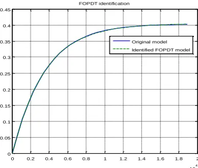
𝐺𝐹𝑂𝑃𝐷𝑇(𝑠) = (1+𝑇𝑠)𝐾 𝑒−𝐿𝑠 (23)
Where, K is referred to as the gain, L is referred as time delay and T is referred as the time constant.
Then, by finding out the step response of the transfer function of the plant (heating furnace) we find out the value of K, L and T.
Where, 𝑇 = 3(𝑇2−𝑇1)
2 , 𝐿 = (𝑇2− 𝑇1) and 𝑎 = 𝐾𝐿
𝑇
Where, T1 and T2 are the time instances in seconds taken from the step response
obtained having a particular steady state gain.
So, the FOPDT model for the plant which is the heating furnace comes out to be, GFOPDT(s) =
0.404272 1 + 3421.93𝑠𝑒
Fig. 2 FOPDT identification, comparison between the original and the identified one which appears to be perfect.
[image:11.595.88.508.424.535.2]Now, on applying Astrom-Hagglund method, Hrone-Reswick 1 and Chien-Hrone-Reswick 2 method,
Table 3 Calculated values Kp, Ki and Kd
Astrom-Hagglund CHR-1 CHR-2
Kp 53.0586 111.005 140.217
Ki 0.109746 0.0231707 0.967806
Kd 1910.28 3779.4 4266.11
The value of λ and μ is being calculated by the Nelder-Mead optimization algorithm separately for both the methods with phase margin = 60o and gain margin = 10dB,
Table 4 Calculated values of λ and μ
Astrom-Hagglund CHR-1 CHR-2
λ 0.10596 0.49282 0.53323
μ 0.010011 0.015107 0.19204
0 0.2 0.4 0.6 0.8 1 1.2 1.4 1.6 1.8 2 x 10
4
0 0.05 0.1 0.15 0.2 0.25 0.3 0.35 0.4 0.45
FOPDT identification
[image:11.595.87.508.627.711.2]Now, the FOPID (PIλDμ) model using the values obtained from and for the Astrom-Hagglund method is,
GAH(s) = 53.0586 +
0.109746
𝑠0.10596 + 1910.28𝑠0.010011 (25)
and, the FOPID (PIλDμ) model using the values obtained from and for the CHR-1 and CHR-2 methods are,
GCHR1(s) = 11.005 +
0.0231707
𝑠0.49282 + 3779.4𝑠0.015107 (26)
GCHR2(s) = 140.217 +
0.967806
𝑠0.53323 + 4266.11𝑠0.19204 (27)
[image:12.595.163.440.377.447.2]Feeding the equation obtained from Astrom-Hagglund method in the closed loop shown in Fig.3 [21], then,
Fig. 3 Closed loop with the plant Gf(s) and FOPID GAH(s)
The output obtained after solving the Fig.3 is, that is the value of GAHO(s) is,
GAHO(s) = 1910.3𝑠
0.11597+53.059𝑠0.10596+0.10975
14494𝑠1.416+6009.5𝑠1.076+1910.3𝑠0.11597+54.749𝑠0.10596+0.10975 (28)
Feeding the equation obtained from CHR-1 method in the closed loop shown in Fig.4, then,
[image:12.595.142.463.622.705.2]The output obtained after solving the Fig.4 is, that is the value of GCHR1O(s) is,
GCHR1O(s) =
3779.4𝑠0.50793+111.01𝑠0.49282+0.023171
14994𝑠1.8028+6009.5𝑠1.4628+3779.4𝑠0.50793+112.69𝑠0.49282+0.023171 (29)
[image:13.595.173.431.221.281.2]Feeding the equation obtained from CHR-2 method in the closed loop shown in Fig.5, then,
Fig. 5 Closed loop with the plant Gf(s) and FOPID GCHR2(s)
The output obtained after solving the Fig.5 is, that is the value of GCHR2O(s) is,
GCHR2O(s) =
4266.1𝑠0.72527+140.22𝑠0.53323+0.96781
14994𝑠1.8432+6009.5𝑠1.5032+4266.1𝑠0.72527+141.91𝑠0.53323+0.96781 (30)
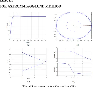
10. RESULT
10.1 FOR ASTROM-HAGGLUND METHOD
Fig. 6 Response plots of equation (28)
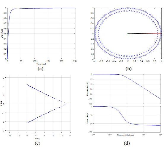
[image:13.595.128.453.406.706.2]10.2 FOR CHIEN-HRONE-RESWICK-1 METHOD
Fig. 7 Response plots of equation (29)
(a) Step response of equation (29), (b) Stability of the system which appears to be stable, (c) Root locus plot of equation (29), (d) Bode plot graph of equation (29)
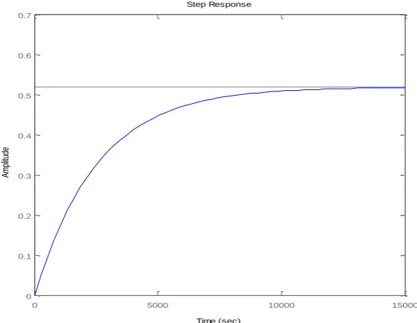
10.3 FOR CHIEN-HRONE-RESWICK-2 METHOD
Fig. 8 Response plots of equation (30)
[image:14.595.159.436.440.688.2]11. DISCUSSION
The Integer Order Model transfer function of heating furnace exhibits very deprived response with a steady state error of more than 50%. Therefore this PID is designed based on the Fractional Order Model of Transfer function. The tuning methods used in above are AMIGO, CHR1 & CHR2. In all these three cases λ & μ are optimized using Nelder-Mead Algorithm. When AMIGO method along with Nelder Mead optimization Algorithm was applied to FOM the final system developed to be stable with a revealed overshoot of merely 3%, where as the settling time also diminished drastically up to 95secs. When CHR1 along with Nelder Meid algorithm was exercised then also system yielded a low overshoot of 4%, and a very swift response with settling time less than 50secs. The system with FOPID tuned by CHR2 & Nelder Meid algorithm exhibited an excellent but slightly lethargic response with nil overshoot, zero steady state error & settling time of 250secs.
12. CONCLUSION
REFERENCES
[1] Daniel Lawson and Glenn Marion, An introduction to mathematical modeling, Bioinformatics and statistics Scotland, (2008) 3-13
[2] George E. Totten and M.A.H. Howes, Steel heat treatment handbook, Marcel Dekker Inc., New York, Basel, 1997
[3] Amlan Basu, Sumit Mohanty and Rohit Sharma, Meliorating the performance of heating furnace using the FOPID controller, Proc. of 2nd international conference on control automation and robotics, Hong Kong, (2016) 128-132 [4] Katsuhiko Ogata, Modern control engineering, fifth edition, PHI learning
private limited, New Delhi-110001, India, 2011
[5] Mohammad Esmaeilzade Shahri and Saeed Balochian, Fractional PID controller for a high performance drilling machine, Advances in mechanical engineering and its applications (AMEA), Vol. 2, No. 4, (2012) 232-235 [6] Amlan Basu, Sumit Mohanty and Rohit Sharma, Ameliorating the FOPID
(PIλDμ) Controller Parameters for Heating Furnace using Optimization Techniques, Indian journal of science and technology, vol. 9 issue 39, (2016) 1-14
[7] Saptarshi Das, Shantanu Das and Amitava Gupta, Fractional order modeling of a PHWR under step-back condition and control of its global power with a robust PIλDμ controller, IEEE transaction on nuclear science, Vol. 58 No. 5, (2011) 2431-2441
[8] Hyo-Sung Ahn, Varsha Bhambhani and Yangquan Chen, Fractional-order integral and derivative controller for temperature profile tracking, Indian Academy of sciences, Sadhana vol. 34, no. 5, (2009) 833–850
[9] H. Vic Dannon, The fundamental theorem of the fractional calculus, and the Meaning of Fractional Derivatives, Gauge Institute Journal, Volume 5, No 1, (2009) 1-26
[10] I. Podlubny, Fractional differential equations – An introduction to fractional derivatives, fractional differential equations, some methods of their solutions and some of their applications, Academic Press, San Diego-Boston-New York-London-Tokyo-Toronto, 1999
[11] YangQuan Chen, Ivo Petr´aˇs and Dingy¨u Xue, Fractional order control - a tutorial, Proc. 2009 American Control Conference Hyatt Regency Riverfront, St. Louis, MO, USA June 10-12, (2009) 1397-1411
[12] Ion V. ION and Florin Popescu, Dynamic model of a steam boiler furnace, The Annals of Dunaera De Jos University Of Galati Fascicle V, Technologies in machine building, (2012) 23-26
International Conference on Mechatronics & Automation, Niagara Falls, Canada, (2005) 216-221
[14] Deepyaman Maiti and Amit Konar, Approximation of a fractional order system by an integer order model using particle swarm optimization technique, Proc. IEEE Sponsored Conference on Computational Intelligence, Control And Computer Vision In Robotics & Automation, (2008) 149-152 [15] Margaret H. Wright, Nelder, Mead and the other simplex method,
Documenta Mathematica Extra Volume ISMP, (2012) 271–276
[16] Neil Kuyvenhove, PID Tuning Methods An Automatic PID Tuning Study with MathCad, Calvin College ENGR. 315, 2002
[17] K. Astrom and T. Hagglund, PID Controllers: Theory, Design and Tuning, The Instrumentation, Systems and Automation Society (ISA), (1995) 20-31 [18] Tepljakov Aleksei, Petlenkov Eduard and Belikov Jurl, A flexible MATLAB
tool for optimal fractional-order PID controller design subject to specifications, Proc. 31st Chinese control system, (2012) 4698-4703
[19] Aleksei Tepljakov, Eduard Petlenkov and Juri Belikov, FOMCON: Fractional-order modeling and control toolbox for MATLAB, Proc. 18th Interntional Mixed Design of Integrated Circuits and Systems (MIXDES) Conference, (2011) 684-689
[20] A. Tepljakov, E. Petlenkov and J. Belikov, FOPID controlling tuning for fractional FOPDT plants subject to design specifications in the frequency domain, Proc. 2015 European Control Conference (ECC), (2015) 3507-3512 [21] A. Tepljakov, E. Petlenkov and J. Belikov, Closed-loop identification of
fractional-order models using FOMCON toolbox for MATLAB, Proc. 14th
![Table 1 CHR 1 method of calculating Kp, Ki and Kd [16]](https://thumb-us.123doks.com/thumbv2/123dok_us/1431875.95729/9.595.90.508.378.514/table-chr-method-calculating-kp-ki-kd.webp)