arXiv:1302.0887v1 [physics.soc-ph] 4 Feb 2013
Edwin Hancock,1,∗ Norio Konno,2,† Vito Latora,3,‡ Takuya Machida,4,§ Vincenzo Nicosia,3,¶ Simone Severini,5,∗∗ and Richard Wilson1,††
1Department of Computer Science, University of York,
Deramore Lane, Heslington, York, YO10 5GH, UK
2Department of Applied Mathematics, Faculty of Engineering,
Yokohama National University 79-5 Tokiwadai, Hodogaya, Yokohama, 240-8501, Japan
3School of Mathematical Sciences, Queen Mary,
University of London, Mile End Road, London E1 4NS, UK
4Meiji Institute for Advanced Study of Mathematical Sciences,
Meiji University, 1-1-1 Higashi Mita, Tama, Kawasaki, Kanagawa 214-8571, Japan
5Department of Computer Science, and Department of Physics & Astronomy,
University College London, Gower Street, London WC1E 6BT, UK
We propose a network growth algorithm based on the dynamics of a quantum mechanical system co-evolving together with a graph which is seen as its phase space. The algorithm naturally generalizes Barab´asi-Albert model of preferential attachment and it has a rich set of tunable parameters – for example, the initial conditions of the dynamics or the interaction of the system with its environment. We observe that the algorithm can grow networks with two-modal power-law degree distributions and super-hubs.
∗Electronic address: [email protected] †Electronic address: [email protected]
‡Electronic address: [email protected] §Electronic address: [email protected] ¶Electronic address: [email protected] ∗∗Electronic address: [email protected]
Models of graph growth are important for studying and simulating the behaviour of a large variety of real-world phenomena and for the in silico construction of networks with desirable properties. Such phenomena occur ubiquitously in the social sciences, technology, and nature (see, for example, [22, 38], for overviews on complex networks). Many pages have been written around the topic of graph growth [13]: among the most extensively studied models are those based on preferential attachment – or “the rich get richer”scheme – together with its many variations. Predating networks science, the basic idea behind preferential attachment goes back to the 1920s and the work of the statistician Yule [47]. The set up usually consists of two ingredients: an iterative process in which new nodes are added sequentially; and a mechanism for choosing neighbours. Only when the preference on the neighbours is a linear function of the degrees of the nodes, then the degree distribution of the growing graph turns out to be a power-law. The literature contains many variants of preferential attachment, respectively defined by local rules, fitness, redirection, copying, substructures, games, geometry, etc. [44].
We are interested in generalizing preferential attachment with steps specified by random walks [7]. The original illustrated in [40] and [29] is simple. Imagine a walker moving along the edges of a graph. At a given node, the walker chooses to stay where it is or to move to one of the neighbouring nodes with a fixed but arbitrary probability. If we wait long enough, the probability that the walker is at a specific node is proportional to the number of its neighbours: this probability converges towards a unique stationary distribution and is independent of the starting node – a fundamental property in algorithmic applications of Markov chains [35, 41]. Once we are close enough to the stationary distribution, we add a new node to the graph, and choose its neighbours according to the distribution induced by the walker. If we keep adding nodes in this fashion, we eventually grow a graph whose degree distribution follows a power-law. When the walker makes an unbiased choice at each node, this mechanism produces exactly the Barab´asi-Albert (BA) random graph [11], which is the most widely studied outcome of preferential attachment so far.
Graph growth fits into a larger picture: the study of dynamical graphs, i.e., graphs changing in time. This is a direction that is currently generating interest as a natural development of static network theory ([28] is a recent review). Letting the structure of a graph co-evolve together with a dynamical process is a particularly appealing and well-motivated idea. In particular, the existence or activity of a node and the strength of a link can be time-dependent on the state of a dynamical process taking place on the graph. For instance, if the nodes of a graph represent individuals having an opinion which changes over time according to a certain rule, and the links stand for friendship among nodes, then the existence and strength of each link can change over time as a function of the difference of opinion between adjacent nodes. People usually tend to remain linked with neighbours who share similar opinions, and to severe links to other individuals having different opinions. In this case the structure of the network depends on the distribution of opinions and, on the other hand, the opinion dynamics depends on the actual connection pattern. In a single word, the network and the opinion formation process are co-evolving. Opinion formation is of course only a very specific example of a process able to drive the evolution of a network. Many other models of networks co-evolving with synchronization [10], diffusion [9], and voter models [15, 45] have been discussed in the last decade (see [26]).
certain circuits with two-qubit gates – have been studied in relation to entanglement distri-bution [2].
With the aim of designing a new methodology to construct networks, we ask the following question: what happens when we consider a graph whose growth depends on the state of a quantum mechanical system? In particular, we are interested in replacing the walk that gives the BA random graph with a quantum dynamics. At each step of the growth process, the neighbours of the newly added node are chosen by observing the state of the quantum system – by using a standard (von Neumann) measurement. We have the co-evolution of two processes: each step of the graph growth process depends on a quantum dynamics and, conversely, the dynamics takes place in a phase space (the graph) modified during the growth.
Quantum walks are an extensively studied area: a continuous version is discussed in [24] and dates back to 1964; a discrete version was introduced in the 1990’s [3]. During the past decade, quantum walks have acquired an important role in the context of quantum computation as a methodology for designing algorithms [8, 33]. Quantum walks are also essential in modeling quantum buses for the transfer of information in nanodevices. The dynamics of an exciton in a spin chain or an arbitrarily coupled spin system is modeled by a coherent quantum walk [16, 20]. Additionally, the transport of energy in large molecular complexes has been explained using a class of quantum walks whose evolution is assisted by interactions of the system with a noisy environment [39].
The quantum walker, like the classical (i.e., random) one, induces a probability distri-bution on the nodes of a graph. However, the distridistri-bution is obtained by measuring the state of the system at a given time. In quantum mechanics the state (of a closed system) is identified with a unit vector in a complex phase space, with probabilities substituted by amplitudes. A major property of quantum walks is the existence of interference effects during the dynamics. Once the position of the quantum walker is measured, the resulting probability distribution is the result of an interference pattern. Notably the distribution does not converge in time because the evolution of a quantum mechanical system is com-pletely reversible [3, 21]. The dynamics can be periodic, or quasi-periodic, but there is no convergence unless we take a time-average [4] – or we stop the evolution at a given time. Interference is one of the ingredients that permits algorithms of good performance to be de-signed [1] and is also responsible of many counterintuitive behaviours of quantum systems. For instance, transporting a packet of information from one node to another node without error, even if routed “randomly” through the graph – a phenomenon called perfect state transfer [20]; or reaching far away nodes with an average probability that is exponentially higher than that for the classical analogue [18]. It is also remarkable that quantum walks have been successfully implemented through various experimental schemes involving light or matter [12, 34, 42].
Here we work withcontinuous-time quantum walks (CTQW) [25]. In these processes the matrix defining network links is interpreted as the system Hamiltonian: this is the operator corresponding to the total energy of the system. The Hamiltonian specifies the interactions between the particles associated with the nodes in terms of coupling strengths. CTQWs are reversible by definition, since the dynamics is governed by the Schr¨odinger equation. (A formal definition is in Appendix.)
drasti-cally influences the distribution of attachment probabilities; moreover, different attachment probabilities depend on the initial node. This reflects the richer behaviour of quantum walks with respect to random walks. We consider the time-average of all distributions obtained by running the walk for a given time. At each step of the iteration, we could choose the distri-bution obtained by stopping the walk at a time determined by a function of the number of nodes. We choose here (arbitrarily) to run the walk for an infinite time – this is like stopping the walk at a random time and it looks like a good choice for exploring the general idea. The time length of each walk is in fact a tunable parameter, differently from the classical BA model.
We consider three alternatives for the location of the starting node used to seed the quantum walk: a) the walks always start from the initial node, i.e. the node added at the first step of the graph growing iteration; b) the walks always start from the node added at the last step; c) at each step, the starting node is chosen at random – of course, we could consider any probability distribution on the set of existing nodes. Since the growth is driven by the quantum walk which effectively acts as a “controller”, we expect different asymptotic distributions. On the one hand, obtaining the time-average of a CTQW is tractable problem; but on the other hand, predicting the properties of our growing graphs is a difficult one because the time-average has erratic behaviour [23]. Presenting an analytic treatments of the asymptotics remains open.
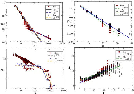
As summarized in Figure 1, different choices of the starting node produce graphs with different structural properties. For(a), the final graph is characterized by a two-mode power-law degree distribution (upper left panel) and hassuper-hubs,i.e. nodes with degree of the same order of the total number of nodes. Such exceptionally highly-connected nodes are usually among the oldest ones, i.e. the nodes added in the very first steps of the iteration. The super-hub turns out to be incident with up to 30% of the total number of edges in the final graph. This condensation phenomenon is indeed observed in real communication and information networks, including the Internet and the World Wide Web, and in biological networks [13]. Notice that the degree distribution obtained in (a) is different from that obtained for the BA random graph shown in the same panel. An obvious by-product of the existence of a super-hub is that the average length of the shortest paths between the nodes is much smaller than the one observed in the Erd˝os-Renyi (ER) and BA random graphs of the same size, as highlighted below.
The final graph also exhibits a surprisingly high local cohesion. This corresponds to a relatively high clustering coefficient (denoted by C), a property which is extensively found in real networks but is rarely reproduced in models of random graphs without introducing artificial ingredients. Another remarkable property is the presence of pronounced disassor-tative degree-degree correlations: the average degree dk of the neighbours of a node with degree k depends on k and decreases as a power-law, dk ∼ kν, with ν = −0.92. The exis-tence of disassortative degree-degree correlations is partially due to the fact that the degree distribution of the resulting graphs do not have a structural cut-off [14], so that the average degree of the neighbours for a substantial fraction of the nodes (i.e., those nodes which share an edge with the super-hub), is dominated by the degree of the super-hub. For comparison, we report in the same panel the value of dk for the BA random graph, which is practically independent of k, except for the boundary effects observed for high values of k.
1 10 100 1000 10000
d
10-6
10-4
10-2
100
P(d)
first ~ k -3.8
~ k-1.0
BA ~ k-2.92
0 10 20 30 40
d
1e-05 0.0001 0.001 0.01 0.1 1
P(d)
last ~ e-0.32 k rnd ~ e-0.26 k
1 10 100 1000 10000
k
1 100
d
k
first k-0.78 BA ~ e-0.0033
0 5 10 15 20 25 30
k 5
10 15
dk
[image:5.612.85.521.71.375.2]last ~ 0.31 k rnd ~ 0.24 k
FIG. 1: The structural properties of the final network heavily depend on the choice of the starting node for the quantum walks. If the walks starts from the node used to seed the growth process (upper left panel), we get a two-mode power-law degree distribution. Here there is a non-negligible probability of forming a super-hub which condenses a large fraction of the edges of the network. In this case, the final network also has pronounced disassortative degree-degree correlations (lower left panel). Conversely, if the walk starts from the lastly added node, or from a randomly selected one, then the degree distribution of the final network is instead exponential (upper right panel). In this case there is a slightly assortative degree-degree correlations (lower right panel). The results are based on 20 realizations withN = 3000 nodes andK= 9000 edges for each scenario.
to be more homogeneous: the final graph has neither hubs nor super-hubs, it exhibits a neg-ligible clustering coefficient and an average shortest path length (denoted by ℓ) comparable to that of an ER or a BA random graph with an equal number of nodes.
As mentioned above, CTQWs have reversible dynamics and the (von Neumann) entropy of any state during the evolution is zero. The dynamics changes if we include an interac-tion between the system and its environment. This introduces decoherence, a phenomenon responsible for the quantum-to-classical transition. Due to decoherence effects, the system becomes thermodynamically irreversible. There are various ways to model decoherence in quantum walks, for example, by monitoring the evolution at a certain rate. The non-zero probability of performing measurements can be interpreted as a weak coupling between the quantum system and a Markovian environment. (See [31] for a detailed survey of the topic.) Generally, when we increase the decoherence rate, the quantum features disappear and after a critical point the behaviour of the system is classical. Thus, in the case of a fully deco-hered quantum walk, we are able to recover the familiar preferential attachment induced by classical random walks [11, 40] – a random walk can be also obtained algorithmically from a CTQW [19]. We can interpolate between these two modes by turning the level of decoherence up or down [17, 32]. For very high decoherence rates, the system will tend to remain in the initial state due to the quantum Zeno effect [5]. This phenomenon can be arguably used to influence the behaviour of the degree sequence by choosing the node from which starting each walk.
Acknowledgments. Part of this work has been done at the Kavli Royal Society Interna-tional Scientific Centre during the workshop “Function Prediction in Complex Networks” (28-29 May 2012). We are grateful to Gorjan Alagic, Andrew Childs, Vivien Kendon, and Andrea Torsello, for useful discussion.
[1] S. Aaronson, A. Ambainis, Proc. IEEE FOCS’01, 2001, 200. [2] A. Ac´ın, J. Cirac, and M. Lewenstein,Nature Phys. 3, 256 (2007).
[3] Y. Aharonov, L. Davidovich, and N. Zagury, Phys. Rev. A 48, 1687 (1993).
[4] D. Aharonov, A. Ambainis, J. Kempe, U. Vazirani,Proc. ACM STOC’01, 2001, p. 50-59. [5] G. Alagic, A. Russell, Phys. Rev. A72, 062304 (2005).
[6] R. Albert, A.-L. Barab´asi,Rev. Mod. Phys.74,, 47 (2002).
[7] D. Aldous, J. Fill, Reversible Markov Chains and Random Walks on Graphs,
http://stat-www.berkeley.edu/users/aldous/RWG/book.html
[8] A. Ambainis, Int. J. Quantum Inf.,1:507-518, 2003.
[9] T. Aoki and T. Aoyagi, Phys. Rev. Lett.109, 208702 (2012).
[10] S. Assenza, R. Gutierrez, J. Gomez-Gardenes, V. Latora, S. Boccaletti, Sci. Rep.1, 99 (2011). [11] A.-L. Barab´asi and R. Albert,Science 286, 509 (1999).
[12] I. Bloch, Nature 453, 1016 (2008).
[13] S. Boccaletti, V. Latora, Y. Moreno, M. Chavez, D.-U. Hwang, Phys. Rep. 424:4-5 (2006), 175–308.
[14] M. Bogu˜na, R. Pastor-Satorras, A. Vespignani,Eur. Phys. J. B 38, 205 (2004). [15] G. A. B¨ohme and T. Gross, Phys. Rev. E 85, 066117 (2012).
[16] S. Bose, Phys. Rev. Lett.91, 207901 (2003).
[17] T. A. Brun, H. A. Carteret, and A. Ambainis, Phys Rev. Lett.91, 130602 (2003).
[18] A. M. Childs, R. Cleve, E. Deotto, E. Farhi, S. Gutmann, and D. A. Spielman, Proc. ACM STOC’03, 2003, pp. 59-68
[20] M. Christandl,et al.,Phys. Rev. Lett. 92, 187902 (2004).
[21] P. A. M. Dirac,The principles of quantum mechanics, 4th Edition (Oxford University Press, 1958).
[22] S. N. Dorogovtsev and J. F. F. Mendes, Evolution of Networks: From Biological Nets to the Internet and WWW (Oxford University Press, 2003).
[23] C. Godsil, March 2011. arXiv:1103.2578v3 [math.CO].
[24] R. P. Feynman, R. B. Leighton, and M. Sands, The Feynman Lectures on Physics, volume III, Addison-Wesley (1965).
[25] E. Farhi, S. Gutmann, Phys. Rev. A58, 915 (1998).
[26] T. Gross and B. Blasius,J. R. Soc. Interface 5, 259-271 (2008).
[27] A. Hamma, F. Markopoulou, S. Lloyd, F. Caravelli, S. Severini, K. Markstrom, Phys. Rev. D
81, 104032 (2010).
[28] P. Holme, J. Saram¨aki,Phys. Rep.,519:3 (2012) 97–125. [29] N. Ikeda,J. Phys. A: Math. Theor. 41(2008 ), 235005.
[30] L. Lov´asz, Random walks on graphs: a survey,Combinatorics, Paul Erd˝os is Eighty (Volume 2), Keszthely, Hungary (1993), 1-46.
[31] V. Kendon,Math. Struct. in Comp. Sci 17(6), 1169-1220 (2006). [32] V. Kendon and B. Sanders, Phys. Rev. A71, 022307 (2004).
[33] N. Konno, In: Franz, U., Schurmann, M. (eds.) Quantum Potential Theory, Lecture Notes in Mathematics, pp. 309–452. Springer-Verlag, Berlin Heidelberg (2008).
[34] J. Mejer, et al.,Nature 449, 443 (2007).
[35] R. Motwani and P. Raghavan, Randomized Algorithms, Cambridge Uiversity Press (1995). [36] M. E. J. Newman,Phys. Rev. E 67,, 026126 (2003).
[37] M. E. J. Newman,SIAM Rev. 45,, 167-256 (2003).
[38] M. Newman, A.-L. Barab´asi, and D. J. Watts,The Structure and Dynamics of Networks (The Princeton Press, 2006).
[39] P. Rebentrost, M. Mohseni, I. Kassal, S. Lloyd and A. Aspuru-Guzik,New J. Phys.11, 033003 (2009).
[40] J. Saram¨aki, K. Kaski, Physica A 341, 80-86 (2004).
[41] A. Sinclair, M. Jerrum, Proc. 20th ACM STOC’88, 1988, pp. 235–244. [42] A. Schreiber,et al.,Science 336, 55 (2012).
[43] A. V´azquez, R. Pastor-Satorras and A. Vespignani, Phys. Rev. E 65,, 066130 (2002). [44] A. V´azquez, Phys. Rev. E 67, 056104 (2003).
[45] F. Vazquez, V. M. Egu´ıluz, and M. S. Miguel,Phys. Rev. Lett. 100, 108702 (2008). [46] D. J. Watts and S. H. Strogatz, Nature 393, 440–442 (1998).
Appendix
Quantum walks
In what follows, agraphG= (V, E) is an ordered pair, whereV(G) is a set whose elements are called nodes and E(G)⊆V(G)×V(G) is a set whose elements are called edges. Since we consider graphs growing over time, we denote byGt = (V, E) the configuration of nodes and edges at time t. Notice that the time of the growth is a discrete variable which is increased by one for each new node added to the graph. Consequently, the graph Gt has exactly tnodes. Thelazy walk matrix on a graph at timet,Gt = (V, E), is (or, equivalently, is induced by)W(Gt) = 12(It+A(Gt) ∆ (Gt)−1), whereIt is thet×tidentity matrix,A(Gt) and ∆ (Gt) are the adjacency matrix and the degree matrix of Gt, respectively. Recall that [A(Gt)]i,j = 1 if {vi, vj} ∈E(Gt) and [A(Gt)]i,j = 0, otherwise; [∆ (Gt)]i,j =δi,jd(i), where d(vi) := |{vj : {vi, vj} ∈ E(Gt)}| is the degree of vi, and δi,j is the Kronecker delta. The
rule of the walk at the t-iteration is Ws(Gt)−→v i 7−→
− →
ψs, where −→vi is an element of the standard basis ofRt and −→ψs ∈Rt. The matrixWs(Gt) induces a distribution on the nodes
of Gt. The j-point of the distribution corresponds to the probability of finding the walker at node vj at time s if the walk started at time 0 from node vi. Thus, the probability is
P[i→j, s] =h−→v j,−→ψsi.
Independently of the initial state, the lazy walk W(Gt) converges to a unique stationary (probability) distribution π(Gt), such that [π(Gt)]i = d(i)/2|E(Gt)|, for each i = 1, ..., t (see, e.g., [30]). Convergence is guaranteed by the stochasticity of W(Gt) and by the fact that there is a non-zero probability for the walker to remain at each node. The rate of convergence depends on the spectral gap of the adjacency matrix.
The stationary distribution of a lazy walk on G2 is clearly the vector π(G2) = 12[1,1]T. When adding v3 to G2, we define P[{v1, v3} ∈E(G3)] = P[{v2, v3} ∈E(G3)] = 12, which follows fromπ(G0). More generally, when adding a nodevt+1 toGt, we attachvt+1 tom ≥1 nodes in Gt, so that the probability of attaching vt+1 tovi reads P[{vt+1, vi} ∈E(Gt+1)] = [π(Gt)]i. The parameter m is fixed but arbitrary. It is important to remark that m is not necessarily the degree of node vt+1 at the end of the growth process which may occur at a time T > t. When m >1 we usually start the growth from a (connected) graphGm.
This mechanism constructs exactly the scale-free graphs for the original version of the Barab´asi-Albert (BA) model [11]. In the BA model, bypassing the walk, a nodevt+1of degree m is added at time t. The probability that vt+1 is adjacent to vi is in fact P[{vt+1, vi} ∈ E(Gt+1)] = [π(Gt)]i =d(i)/2|E(Gt)|, which is exactly the stationary probability of finding a lazy random walker in Gt at node vi.
By generalizing the above picture, given a graph ontnodes,Gt, we define a unitary matrix U(s, t) =e−iA(Gt)s, wheres ∈R+. Unitary means thatU(s, t)U†(s, t) =U†(s, t)U(s, t) =
I, where I is the identity matrix and U†(s, t) is the adjoint of U(s, t). In this case the dynamics is reversible / non-dissipative because of unitarity. The matrix U(s, t) defines a
continuous time quantum walk (CTQW) onGt [8]. Therule of the CTQW at thet-iteration is U(s, t)|vii 7−→ |ψsi, where |vii is an element of the standard basis of a formal Hilbert space H ∼= Ct and |ψsi ∈ H. The Dirac notation tells that k|ψsik = 1. The probability that at times the walker visits a node vj starting in a node vi is P[i→j, s] =|[U(s, t)]i,j|2.
This probability is obtained by a projective measurement on |ψti: P[i→j, s] = |hvj|ψti|2.
of quantum mechanics the post-measurement state is the observed standard basis vector. The matrix A(Gt) is interpreted as the Hamiltonian inducing the quantum mechanical evolution of a particle whose degrees of freedom of the dynamics are constrained on the edges of Gt. Indeed, this can be seen as the operator describing the evolution of the single excitation sector of a quantum spin system (XY model) in virtue of the Jordan-Wigner transformation [16].
At the t-th iteration, the mixing matrix of the CTQW at time s is defined by
Ms,t =eiA(Gt)s
◦e−iA(Gt)s
=U(s, t)◦U(−s, t),
where [A◦B]i,j := [A]i,j·[B]i,j denotes the Schur-Hadamard product of two matricesA and B. The matrix Ms,t depends on s; it gives the instantaneous mixing behaviour of the walk. Formally, an element ofMs,t is constructed by multiplying together the amplitudes obtained by evolving the system for a time s in the future and for a time s in the past. Differently from the case of a lazy random walk, here there is never convergence, because the dynamics is non-dissipative. For the walk, we have k|ψsik =kU(s, t)|viik= 1.
We could also define an instantaneous mixing time by looking at the smallest s ∈ R+
for which the probability induced by the CTQW is close in some measure of similarity (for example, total variation distance) to the uniform or the stationary probability distribution. A possibly different growth model can be defined by making use of the distribution obtained at a given time s. In this case, the growth is entirely dependent on the chosen value of s; this could be fixed for each t or as a function of t, for instance. To avoid a dependence on s, we consider a time-average of Ms,t.
The average mixing matrix is defined by taking a Cesaro mean:
c
Mt= lim s→∞
1 s
Z s
0
eiA(Gt)s
◦e−iA(Gt)s
ds=X j
Ej,t◦2,
where Er is the r-th idempotent of the spectral decomposition of A(Gt) = PjλjEj. In other words, Ej,t represents the orthogonal projection onto the eigenspace ker(A(Gt)−λjI), where λj is the j-th eigenvalue of A(Gt). The ij-th entry of Mtc is the average probability that a walker is found at node vj (starting at node vi). Remarkably, Mtc is rational [23].
In our model of growth based on CTQWs, the attaching probability is defined by
P[{vt+1, vj} ∈ E(Gt+1)] = [Mt]i,jc , if we assume that the walker started from node vi at
the t-th iteration of the growth process. Depending on the starting node vi, we get a dif-ferent attaching probability which will be completely defined by Gt. The time length of the walk is not relevant given that Mtc is defined as a limit for s → ∞.
LetKndenote thecomplete graphonnvertices. This is the unique graph withn(n−1)/2 edges. Let [A]i the i-th row of a matrix A.
Algorithm. The growth of a graph based on CTQWs starts with Gm = Km. Then, for
everyt > m, we samplemneighboursvj1, vj2, ..., vjmof the new nodevtfrom the distribution
[Mtc−1]i and create m edges {vt, vj1},{vt, vj2}, ...,{vt, vjm}.
randomly sampled node for each step of the algorithm. The initial condition Gm =Km can be also relaxed.
This simple growth algorithm, based on the sampling of new edges according to the time-average of the attaching probability distribution, suffers from the fact that the evaluation of the Cesaro mean requires the full spectrum of the adjacency matrixA(Gt). This is the critical step. In fact, although efficient schemes exist to compute the few largest eigenvalues of a symmetric matrix of size n, the time complexity of the computation of the whole spectrum is ∼O(n3). At a first analysis, it follows that the number of steps needed to sample graph of t nodes constructed with our method is of the order O(t3). Sampling a CTQW-based graph is much more costly than sampling a BA random graph, for which the most efficient algorithm runs in O(t).
Network-theoretic parameters
Let G = (V, E) be a graph on n nodes {v1, v2, ..., vn}. The average degree of G is d(G) =Pni=1d(vi). Letd(vi) = k, for a given nodevi ∈V(G); then theaverage degree of the neighbours ofvi is denoted bydk. We say that two nodesvi, vj ∈V(G) areconnected if there isl∈Z+such that [Al(G)]i,j >0. Equivalently,viandvj are connected if there is a walk form vi to vj. A walk from vi to vj is a sequence of edges {{vi = i0, i1},{i1, i2}, . . . ,{in−1, in = vj}}, where the nodes are not necessarily all distinct. When the nodes of a walk are all distinct then the we call it a path. The length of a path is the number of edges in the path. The distance d(i, j) between vi, vj ∈ V(G) is defined as the length of the path from vi tovj with the minimum number of edges. The average shortest path length of G is then defined as ℓ := n(n1−1)Pi,jd(i, j). If there is no path containing vi and vj then d(i, j) =∞, by convention. Consequently, ℓ is finite only for connected graphs, i.e. when every pair of nodes of the graph is contained in a path. The graphs generated by the algorithm are connected by construction. The clustering coefficient Ci of a node vi ∈ V(G) is a measure of the local cohesion at vi. Taking k = d(vi), we have Ci := k(k1−1)T(vi), where T(vi) is the number of different triangles containing vi. A triangle is a graph of the form ({vi, vj, vk},{{vi, vj},{vj, vk},{vi, vk}}). Theclustering coefficient ofGis the average of the clustering coefficients of all nodes: C = n1 PiCi (See [37] for a general reference on these notions).
Real networks usually exhibit correlations in their structure. For instance, in some net-works (mostly social, information and communication netnet-works) high-degree nodes are pref-erentially linked to other high-degree nodes, while in biological and technological networks high-degree nodes are preferentially linked to low-degree nodes [38]. The existence of degree-degree correlations can be quantified in different ways. One of the most common methods is by computing dk as a function of k. If a graph is uncorrelated then the degree of the neighbours of a node of degree k does not depend on k, and it is possible to show that dk =hk2i/hki. In real networks we observe thatdkdepends on k: if dk increases whenk de-creases, we say that the network has assortative degree-degree correlations; on the contrary, if dk decreases when k increases, we say that the network has disassortative degree-degree correlations. (See [36] for an in-depth discussion about degree correlations in networks.) In most real networks, dk ∼ kν (with a little abuse of notation) and the exponent ν can be effectively used to quantify degree-degree correlations: ν > 0 and ν < 0 define assortative