This is a repository copy of
Model predictive control system design and implementation for
spacecraft rendezvous
.
White Rose Research Online URL for this paper:
http://eprints.whiterose.ac.uk/90483/
Version: Accepted Version
Article:
Hartley, E., Trodden, P., Richards, A. et al. (1 more author) (2012) Model predictive control
system design and implementation for spacecraft rendezvous. Control Engineering
Practice, 20 (7). 695 - 713. ISSN 0967-0661
https://doi.org/10.1016/j.conengprac.2012.03.009
[email protected] Reuse
Unless indicated otherwise, fulltext items are protected by copyright with all rights reserved. The copyright exception in section 29 of the Copyright, Designs and Patents Act 1988 allows the making of a single copy solely for the purpose of non-commercial research or private study within the limits of fair dealing. The publisher or other rights-holder may allow further reproduction and re-use of this version - refer to the White Rose Research Online record for this item. Where records identify the publisher as the copyright holder, users can verify any specific terms of use on the publisher’s website.
Takedown
If you consider content in White Rose Research Online to be in breach of UK law, please notify us by
Model Predictive Control System Design and Implementation for Spacecraft
Rendezvous
E. N. Hartleya,∗, P. A. Troddenb,1, A. G. Richardsb, J. M. Maciejowskia
aUniversity of Cambridge Department of Engineering, Trumpington Street, Cambridge. CB2 1PZ. United Kingdom. bDept. of Aerospace Engineering, University of Bristol, Queens Building, University Walk, Bristol. BS8 1TR. United Kingdom.
Abstract
This paper presents the design and implementation of a model predictive control (MPC) system to guide and
control a chasing spacecraft during rendezvous with a passive target spacecraft in an elliptical or circular orbit, from
the point of target detection all the way to capture. To achieve an efficient system design, the rendezvous manœuvre
has been partitioned into three main phases based on the range of operation, plus a collision-avoidance manœuvre to
be used in event of a fault. Each has its own associated MPC controller. Linear time varying models are used to enable
trajectory predictions in elliptical orbits, whilst a variable prediction horizon is used to achieve finite-time completion
of manœuvres, and a 1-norm cost on velocity change minimises propellant consumption. Constraints are imposed to
ensure that trajectories do not collide with the target. A key feature of the design is the implementation of non-convex
constraints as switched convex constraints, enabling the use of convex linear and quadratic programming. The system
is implemented using commercial-off-the-shelf tools with deployment through the use of automatic code generation in
mind, and validated by closed-loop simulation. A significant reduction in total propellant consumption in comparison
with a baseline benchmark solution is observed.
Keywords: Autonomous vehicles; constraints; embedded systems; model-based control; optimization; path planning; predictive control; spacecraft autonomy
1. Introduction
Rendezvous is an important part of current and future space missions. For example, in the Mars Sample Return
(MSR) mission (R´egnier et al.,2005;Mura,2007;Beaty et al.,2008) there will be a rendezvous and capture
manœu-vre, where a soil sample, enclosed in a passive container, must be captured by an orbiting chaser craft. Due to the
distances involved, and the resulting communication delays (up to 20 min in each direction), in combination with the
levels of accuracy required to correctly perform the capture (tolerance of approximately 20 cm) there is a particularly
strong motivation to perform this operation autonomously.
∗Corresponding author
Email addresses:[email protected](E. N. Hartley),[email protected](P. A. Trodden), [email protected](A. G. Richards),[email protected](J. M. Maciejowski)
This paper describes the design and implementation of a Model Predictive Control (MPC) system (e.g.
Ma-ciejowski(2002);Camacho & Bordons(2004);Rawlings & Mayne(2009)) for the rendezvous and capture associated
with the MSR mission, carried out as part of the ESA ORCSAT (On-line Reconfiguration Control System and
Avion-ics Technologies) project. The MPC control system is designed to be used from the point of target detection to the
point of target capture and to function in both circular and elliptical orbits.
Whilst MPC has its origins in the process industries (Qin & Badgwell,2003), it has recently been applied to
vehicle manœuvre trajectory planning problems (including short-range spacecraft rendezvous scenarios (Richards
& How,2003a;Larsson et al.,2006;Breger & How,2006), UAV scenarios (Shim et al.,2003; Richards & How,
2006;Almeida,2008), spacecraft formation flying scenarios (Manikonda et al.,1999; Breger & How,2007), and
spacecraft attitude control applications (Manikonda et al.,1999;Hegrenæs et al.,2005;Wood & Chen,2008)). In
addition,Bodin et al.(2011) indicates that the MPC formulation ofLarsson et al.(2006) has been used successfully
for trajectory tracking on a real test mission.
Unlike the works mentioned above, which have focused on application of MPC to individual spacecraft
manœu-vres or to tracking problems, this work considers the use of MPC end-to-end from the point of target detection all
the way until target capture. The design presented explicitly considers implementation of MPC within the constraints
of a spacecraft avionics architecture, although this paper focuses purely on the MPC design aspects of the ORCSAT
project.
Since minimising propellant consumption is critical to space operations, a controller based on optimising fuel
usage is attractive. It follows naturally from early work on trajectory optimisation (Hohmann,1925;Kaplan,1976;
Prussing,1991;Battin,1999) to move the optimiser onboard the spacecraft in order to circumvent communication
delays. The HARVD control system (Kerambrun et al.,2008) goes some way towards this by selecting guidance
trajectories and nominal control actuation sequences from a large library of pre-computed optimal manœuvres. These
are augmented with corrective manœuvres based on current navigation information to ensure faithful tracking of the
desired paths.
Model predictive control possesses some attractive characteristics as a candidate guidance and control framework.
Firstly, because model predictive control re-plans the optimal trajectory at each sampling instance, it is conceivable
that propellant consumption in the presence of uncertainty could be reduced in comparison to tracking a pre-computed,
nominal trajectory as performed by HARVD and on the state-of-the-art Automated Transfer Vehicle (ATV) (Ganet
et al.,2002). Secondly, due to the implicit way in which the MPC problem is specified, carrying an exhaustive library
of manœuvres for every possible initial configuration is not necessary. Thirdly, rendezvous operations typically have
many constraints, including limited thruster capability, sensing regions, requirements for safe operation limits and
so on. The intrinsic ability of MPC to handle constraints, and the ability to consider the control objective to be
achievement of a trajectory end-point rather than a complete trajectory, alongside the availability of well-researched
models of relative dynamics that can be used for prediction (Clohessy & Wiltshire,1960;Tschauner,1967;Carter,
& How,2007) therefore makes it a logical choice for rendezvous.
Other welcome characteristics that can be obtained through the MPC design process include robust finite time
completion (Richards & How,2003b,2006) and guaranteed safe passive abort trajectories (Breger & How,2006,
2008). MPC is also inherently reconfigurable. Constraints (e.g. thrust availability, passive safety requirements), and
model parameters (e.g. target orbit) can be modified on-line — an attractive feature if these are not known exactly
until the target has been detected.
Of course, the flexibility of MPC comes at a cost, and the main challenge of deploying MPC for spacecraft is its
complexity. Numerical optimisers are comparatively complex pieces of software, at odds with the limited computing
available on board a spacecraft. One of the key considerations of this work is the integration of MPC into an avionics
architecture and software toolchain.
2. Mission Information
The mission scenario that will be considered in this paper is representative of one possible realisation of the Mars
Sample Return mission (Beaty et al.,2008), where the “target” vehicle contains the soil sample to be captured and
returned by the “chaser”. MPC is applied to provide trajectory guidance and control for the whole rendezvous. During
the final 100 m prior to capture, MPC will also provide small-angle attitude control to maintain the target pointing
necessary for the short-range relative navigation sensor (LIDAR) to function correctly. Before this point, it is assumed
that attitude control will be performed by an independent control system using reaction wheels.
2.1. Nominal Initial Conditions
The control system is designed using two nominal reference scenarios based on possible outcomes of the launch
of the sample capsule. The initial conditions for each of these scenarios are expressed in terms of Keplerian orbital
elements (Kaplan,1976;Sidi,1997; Fehse,2003) in Table1. These drive the design, as they force the candidate
control system to handle both circular and elliptical orbits. In each case, the chaser starts approximately 300 km
away from the target — a distance corresponding to the approximate operating range of the long-range RF relative
navigation sensors.
2.2. Chaser Characteristics
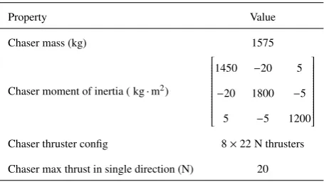
The chaser mass, moment of inertia and maximum thrust are shown in Table 2. Note that maximum thrust
guaranteed in every direction is less than the individual thrust on a single thruster due to the geometric alignment of
the thrusters and the requirement that a zero net torque must be commanded for a pure translation manœuvre.
2.3. Navigation Uncertainty
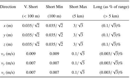
To be of practical use, the MPC controller must cope with the relative navigation uncertainties shown in Table3
Scenario Circular Elliptical
Vehicle Target Chaser Target Chaser
Semi-major axis,a(km) 3893 3843 4643 4593
Eccentricity,e 0 0.003 0.20441 0.20741
Inclination,i(deg) 30.0 30.3 15.0 15.3
RAAN,Ω(deg) 0 0.3 323.4 323.7
Argument of periapsis,ω(deg) 0 0.3 0 0.3
[image:5.595.183.411.510.638.2]True anomaly,ν(deg) 0 -8 0 -5
Table 1: Scenario initial conditions (nominal)
Property Value
Chaser mass (kg) 1575
Chaser moment of inertia ( kg·m2)
1450 −20 5
−20 1800 −5
5 −5 1200
Chaser thruster config 8×22 N thrusters
Chaser max thrust in single direction (N) 20
of error in individual directions by √3 implies the error is defined in terms of 3D Euclidean distance. Division by √2
implies that the error is defined in terms of 2D distance and a worst case error in the third co-ordinate. At short range,
linear interpolation is used between minimum and maximum uncertainty levels.
Direction V. Short Short Min Short Max Long (as % of range)
(<100 m) (100 m) (5 km) (>5 km)
x(m) 0.035/√2 0.035/√2 3/√3 (0.1/√3)%
y(m) 0.035/√2 0.035/√2 3/√3 (0.1/√3)%
z(m) 0.035/√2 0.035/√2 3/√3 (0.1/√3)%
vx(m/s) 0.009 0.009 0.1/
√
3 (0.003/√3)%
vy(m/s) 0.007 0.007 0.1/
√
3 (0.003/√3)%
vz(m/s) 0.007 0.007 0.1/
√
[image:6.595.174.421.171.319.2]3 (0.003/√3)%
Table 3: Navigation uncertainty (3σvalues)
2.4. Simulation
The MPC control system has been developed and tested using a Simplified Rendezvous Performance Simulator
(SRPS) provided by ORCSAT project partners GMV. This includes a full non-linear model of the rigid body dynamics
of the target and chaser in a Mars orbit, and representative thruster models. Navigation signals are simplified, and the
values presented in Table3are used to model navigation uncertainty as zero-mean Gaussian noise. At ranges between
100 m and 5 km, the navigation uncertainty is interpolated between the values presented in Table3.
A further level of validation has been obtained by integrating the final MPC control system developed into a higher
order Functional Engineering Simulator (FES) (Le Peuv´edic et al.,2008a) with more representative sensor models and
authentic navigation filters.
3. System-Level Design
Following detection of the target at a range of approximately 300 km, the control system must transfer the chaser
spacecraft to a “blinding point” approximately 3 m from the target, from which a passive drift trajectory must be
used to complete the capture. The approach must be performed in a passively safe manner — if control authority is
removed (i.e. if the thrusters are disabled due to a fault in the control or navigation systems), the resulting passive
drift trajectory must remain outside of a “safety sphere” centred on the target. An additional operational requirement
is that the chaser must visit a sequence of pre-specified holding points in the neighbourhood of the target and await
authorisation to proceed from ground control.
In order to take greatest advantage of the ability of MPC to perform optimisation and actively handle constraints
func-tionality. Little benefit over use of a classical feedback controller would be expected if MPC were used purely within
an inner-loop to regulate to a pre-determined trajectory. Similarly, tracking a trajectory generated by MPC using a
classical inner-loop controller is not an appealing solution for this application, because “bang-off-bang” actuation
patterns are known to be fuel-optimal under ideal conditions (Sidi,1997;Battin,1999;Fehse,2003), and there is a
need to constrain transient responses as well as steady-state conditions.
Fulfilment of the objective described above using a single MPC controller would require a prediction model
complex enough to perform accurate trajectory propagations over long periods of time, a prediction horizon at least
long enough to predict a trajectory one orbital period into the future and a sampling frequency high enough to achieve
the required accuracy prior to capture. Given that to be a useful engineering solution, the MPC controller must be
evaluated in real-time at each sampling instance, it is evident that these requirements are in conflict. At the other
extreme, it would be possible to have an MPC implementation for a large number of individual manœuvres. However,
this would push up the complexity of development and implementation, and reduce the number of degrees of freedom
with which the MPC could provide improvements.
To obtain a usable and practically realisable control system with good closed loop performance, it was decided to
subdivide the rendezvous into a small number of phases. This allows the prediction model, cost function, constraint
set, sampling period and prediction horizon to be chosen to suit the mission requirements.
3.1. Candidate Prediction Models
There is a significant amount of literature concerning simplified state transition matrices (STM) for propagation
of the relative trajectories of two orbiting objects. The most well-known model is the Hill-Clohessy-Wiltshire (HCW)
equations (Clohessy & Wiltshire,1960), which propagate the relative position and velocity of the chaser with respect
to the target in a Cartesian reference frame centred on a target object in a circular orbit. The HCW equations can be
used to form a linear time-invariant (LTI) state-space model of the relative dynamics. However, the HCW equations
rely on the assumption that the target orbit is near-circular (orbital eccentricitye=0), and that radial and out-of-plane separations are small. As observed byInalhan et al.(2002), the assumption of circular orbit can cause significant
prediction error for orbits of eccentricity as little ase=0.005. In this work, consideration of elliptical target orbits is essential, meaning that the HCW equations are not directly applicable.
As exploited by (Tschauner,1967;Carter,1998;Inalhan et al.,2002;Yamanaka & Ankersen,2002), an otherwise
linear model can be parameterised by the true anomaly of the targetνtgt. Assuming no additional forces perturb the
target orbit, a mapping can be made betweenνtgt and time using Kepler’s equation, thus allowing construction of
an LTV model (Breger,2002). These methods predict in a Cartesian or cylindrical local reference frame and allow
for elliptical orbits, but still assume small radial and out-of-plane separations. The model ofYamanaka & Ankersen
(2002) has the appealing property that, unlike previous models, it is numerically identical to the HCW equations for
The Gim-Alfriend STM (Gim & Alfriend,2003) offers an alternative LTV approach. It uses a linearised
geomet-ric mapping between relative curvilinear coordinates (Melton,2000) and differences in a non-singular set of orbital
elements. It is specifically designed to accurately consider the mean and osculating effects of J2 — the effect of
gravitational variation due to the oblateness of the central body of the orbit.
A further approach is to use Gauss’ variational equalities (GVEs) (Schaub et al.,2000;Breger & How,2007) —
models based on Gauss’ expressions relating an acceleration vector expressed in a local frame to changes in classical
orbital elements. A linear time-varying model is formed by linearising differences in these elements. Relatively
small changes in the orbital elements can lead to relatively large separations in Cartesian space, which is helpful
in minimising the effect of linearisation error using Taylor expansions. Breger & How (2007) show how the
Gim-Alfriend approach can be used with GVEs to include the effects ofJ2.
3.2. Rendezvous Phase Apportionment
In order to achieve the best compromise between flexibility, performance and complexity, the phases chosen
for MPC design are apportioned in a similar way to that done in the baseline control system, HARVD (Kerambrun
et al.,2008). By partitioning the control problem in this way, each MPC controller can be tuned for its respective
rendezvous phase (Figure1), accounting for factors such as the relative importance of control accuracy, maximum
planned trajectory duration and computational demands. The designs are also influenced by the anticipated levels of
navigation uncertainty, and by higher level mission requirements.
3.2.1. Intermediate Range
The first phase, OSTG (Orbit Synchronisation Translational Guidance) uses theJ2modified GVEs as a prediction
model, to accurately capture long range dynamics. Preliminary studies found that for the present application, this
model provided the lowest error between predicted open-loop trajectories, and trajectories simulated using the SRPS.
Short-term control accuracy is not critical during this phase, so a relatively long sampling period can be used to
obtain a relatively long prediction horizon without an excessive number of decision variables in the optimisation
problem. OSTG should bring the chaser from a distance of approximately 300 km (of which the radial and
out-of-plane components will be significant, so would lead to high levels of linearisation error for models based upon
Cartesian or cylindrical co-ordinates) into an orbit with the same Keplerian orbital elements (e.g. Kaplan(1976);
Sidi(1997);Fehse(2003)) as the target, with the exception of the true anomaly, νchs, which should attain a value
corresponding to an in-track separation of between 10 km and 30 km. Unlike in HARVD, in-plane and out-of-plane
corrections are considered simultaneously.
3.2.2. Short Range
The second phase, INTG (Impulsive Nominal Translational Guidance) starts once the OSTG phase has been
com-pleted. At this point, out-of-plane and radial separations are smaller, but there is still a significant in-track separation.
between a series of prescribed holding points up until a target approach point (TAP) approximately 100 m from the
target. At each holding point, the chaser must wait for a signal from ground control indicating permission to
pro-ceed. If the INTG phase commences at a point closer than the furthest-out holding point, the first holding point to be
scheduled should be the nearest one in the direction of the target.
At short range, short-term accuracy is more important than accuracy of long-term trends. The linearised geometric
transformationΣ(etgt) that translates from orbital element separations to distances is only an approximation. It is also
important for the MPC controller to function in an elliptical orbit. In order to accommodate more accurate passive
safety constraints and accurate attainment of holding points, a shorter sampling period is required. To accommodate
these requirements, the prediction model is provided by the Yamanaka-Ankersen equations (Yamanaka & Ankersen,
2002). This is a simpler model than theJ2-modified GVEs, and linearisation error is not significant once the
out-of-plane and radial separations have been mostly corrected.
3.2.3. Very Short Range
The final phase, FTTG (Forced Terminal Translational Guidance) uses the Yamanaka-Ankersen equations and a
linearised quaternion-based attitude model to allow high precision control up until the final capture. Because at this
range the primary relative navigation sensor is LIDAR, it is critical that an attitude orientation is maintained so that the
target is within the LIDAR’s field of view. This can be achieved by regulating to a setpoint which maintains the target
in the centre of the LIDAR field of view. Similarly, the closed-loop trajectory must reach a point so that a capture
error of less than 20 cm is achieved after a subsequent period of free drift. It is therefore clear that during this phase a
far shorter sampling period is required in order to facilitate the necessary level of disturbance rejection.
3.2.4. Collision Avoidance Manœuvre (CAM)
A fourth phase (CAM) for active collision avoidance in case of contingency is included in the design. If a fault
occurs during the FTTG phase, or if it is detected that the velocity or position close to the “blinding point” puts the
chaser on a collision-course with the target, an active avoidance manœuvre must be performed to move the chaser
away from the target. In the case of the scenario considered in this work, the chaser must be moved to a distance at
least 500 m from the target in at most 3 orbits. At this point, the INTG mode can resume operation.
Being a contingency manœuvre, the CAM might need to operate with reduced navigation performance. If
target-pointing is lost, the navigation estimate will degrade over time. Furthermore, to successfully avoid collision, the CAM
must calculate and command a control action in a short period of time from the instant it is triggered. Therefore, for
speed, and because the CAM operates at relative close proximity to the target, the Yamanaka-Ankersen equations are
preferred.
3.3. System Architecture
The MPC subsystems are implemented separately, each in an individual Simulink subsystem, with a set of
Target
Chaser OSTG INTG
FTTG TAP
[image:10.595.200.395.111.221.2]CAM
Figure 1: Rendezvous phases (not to scale)
any support functions required to detect whether the subsystem should be active or not, perform co-ordinate
transfor-mations, detect completion of the mission phase and raise a “success” flag, and, in the case of the INTG mode, choose
which holding point should be achieved next.
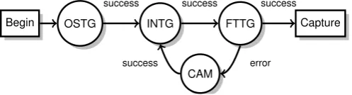
Each of the MPC controller subsystems is responsible for raising a “success” flag when its terminal conditions
have been achieved. An external scheduling algorithm then enables the MPC corresponding to the next mission phase.
The schedule of phases is presented in Figure2. It should be noted that the CAM is only applicable during the final
phase of the rendezvous. In the OSTG and INTG phases the trajectories are naturally passively safe so a “do nothing”
approach is sufficient.
OSTG INTG FTTG Capture
Begin
CAM
success success success
error success
Figure 2: MPC Controller Scheduling
A separate output preparation block, common to all modes and operating at a higher sampling frequency, is also
implemented to convert impulsive velocity change commands generated by the MPC subsystems to finite duration
acceleration pulses and to rotate these pulses from the co-ordinate system preferred by the active MPC subsystem to
an inertial reference frame as determined by the interface with the simulator.
3.4. Optimisation Formulation
One of the key requirements of the work presented here is that the final design must be able to run in real-time on
hardware representative of what could be included on board a future spacecraft. As part of the high-level system design
the MPC for all phases was restricted to linear time-varying dynamics models based upon convex linear programming
(LP) or quadratic programming (QP) with linear constraints. LTI models are unsuitable as they cannot capture relative
dynamics in elliptical orbits — of the available dynamics models, only HCW is LTI and that is only applicable to the
[image:10.595.174.423.415.482.2]the additional complexity in the optimiser. Similarly, solver software for mixed-integer optimisation (Bemporad &
Morari,1999) was judged too complex for this application, despite the potential to handle the non-convex constraints.
Explicit MPC (Bemporad et al.,2002b,a), in which the optimisation is pre-solved offline as a parametric function
of the state was ruled out due to the complex nature of the control law. Explicit MPC can be appealing, because the
control law is typically a piecewise affine function of the state, which is readily implemented. However, with the
LTV dynamics, many complex constraints, six or more states and a large region of operation, that control law would
become prohibitively large in terms of the number of partitions.
The restriction to only use convex LP or QP means that non-convex constraints such as collision avoidance must
be approximated in a convex manner. However, there is no requirement that only a single QP or LP may be solved
at each sampling instance. For example, in order to include a measure of time in the cost function for the OSTG and
INTG phases a variable horizon is used. This can be implemented usingswitched controllers. At each time step each element of a set of convex, finite horizon MPC controllers is evaluated, each with a different prediction horizon up to a
maximum horizonNmax. The control action from the controller with the lowest overall cost (calculated as a weighted
sum of the prediction horizon and the optimum cost from the finite horizon MPC controller) is chosen and applied to
the plant.
4. Intermediate Range (OSTG)
The objective of the OSTG MPC controller is to synchronise the orbit of the chaser with that of the target in finite
time, whilst minimising propellant usage. The chaser should be brought onto the target orbit, with a difference in true
anomaly∆νsuch that the “in-track” separation is between 10 km and 30 km. This may be on either side of the target.
4.1. Prediction Model
For the intermediate range MPC controller (OSTG), a prediction model based on linearisedJ2-modified Gauss’s
Variation Equations (GVEs) (Breger & How,2007) is used. Non-singular orbital elements are used rather than the
basic Keplerian orbital elements, to avoid ambiguities between ω andν when e = 0, and to avoid numerical ill condition when calculating theJ2modification (Gim & Alfriend,2003). Denoting the vector of orbital elements of
chaser and target using subscripts “tgt” and “chs” as
echs=
achs echs ichs Ωchs ωchs νchs
T
(1)
and
etgt=
atgt etgt itgt Ωtgt ωtgt νtgt
T
respectively, the relative non-singular orbital elements (Gim & Alfriend,2003) are expressed as:
∆e=
∆a ∆θ ∆i
∆q1
∆q2
∆Ω =
achs−atgt
(νchs+ωchs)−(νtgt+ωtgt)
ichs−itgt
echscosωchs−etgtcosωtgt
echssinωchs−etgtsinωtgt
Ωchs−Ωtgt
. (3)
The state vector during the OSTG phase is
x(j)= ∆e(j). (4)
An impulsive input discretisation is used, with the plant inputs being expressed as impulsive velocity changes
ex-presssed in the chaser orbital frame (COF). The chaser orbital frame is an LVLH (local vertical, local horizontal)
reference frame centred on the centre of mass of the chaser. The COF axes are defined aszcof pointing towards the
focus of the orbit,ycof parallel to the chaser orbital angular velocity, andxcofcompleting the right-hand set.
4.2. Variable Horizon Cost Function
It has been demonstrated in the literature (e.g. Tillerson et al. (2002)) that a 1-norm cost function offers better
conservation of fuel than a quadratic or sum-of-squares cost function. Therefore, in order to minimise absolute
propellant consumption whilst reaching the desired terminal conditions in finite time, a 1-norm cost function on the
∆Vapplied in the chaser orbital frame is used, along with a weighted variable horizon (Richards & How,2006,2003a). In accordance with the use of variable horizon MPC, the control objectives are encoded in the terminal constraints
(which will be specified later). The chosen cost function to be minimised is
J(u, α,N)=N+wu N−1
X
k=1
ku(t+kTs|t)k1
whereu(t+kTs|t) is interpreted as the predicted input at timet+kTsgiven the measurements at timet,wuis a scalar
tuning parameter weighting the propellant consumption against manœuvre time,N ≤Nmaxis the prediction horizon
(in sampling instances), and
u,
u(t+Ts|t)T . . . u(t+(N−1)Ts|t)T
T
. (5)
Variableαrepresents the angle of a passive safety constraint. Section4.4describes how multiple values are attempted
via switched MPC laws. It should be observed from this structure that the first element of the predicted input sequence
LTV prediction model used conforms to the following structure:
x(t+Ts|t)=A(t)x(t|t)+B(t)u(t|t−Ts) (from prev. time step)
x(t+2Ts|t)=A(t+Ts)x(t+Ts|t)+B(t+Ts)u(t+Ts|t)
x(t+3Ts|t)=A(t+2Ts)x(t+2Ts|t)+B(t+2Ts)u(t+2Ts|t) ..
.
x(t+NTs|t)=A(t+(N−1)Ts)x(t+(N−1)Ts|t) (6)
+B(t+(N−1)Ts)u(t+(N−1)Ts|t).
4.3. Input Constraints
Constraints on the maximum deliverable∆Vare placed on each element of the input vector
−ulim≤ui(j|t)≤ulim, i∈ {1,2,3},
whereulimis defined by the force capacityFc(in Newtons), massm(in kilograms), sampling periodTs(in seconds)
and duty cycleDτ(as a fraction of the sampling period):
ulim=Dτ
Fc
mTs. By setting Dτ ≤ 1/
√
2, this imposed∞-norm constraint can be used to conservatively guarantee satisfaction of a
2-norm constraint on maximum deliverable thrust in any direction.
4.4. Safety Constraints
The orbit synchronisation must be performed in a passively safe manner. The free drift trajectories following any
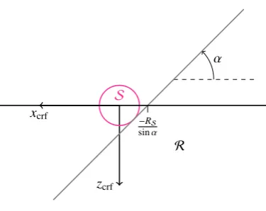
∆Vcommand by the MPC must remain outside of asafety spherecentred on the target for at least one orbital period. This safety sphere is specified to vary in size as a function of the current separation between target and chaser. This,
again is clearly a non-convex constraint. The non-convex safety sphere avoidance constraint can be approximated by
using a rotating half-space constraint (Figure3).
The MPC problem is initially solved with output constraints ensuring that the free-drift trajectories remain inside
the half-space denoted R in Figure3. This is done by including explicit open-loop predictions of the free drift
trajectories at each time step, as originally proposed by (Breger & How,2008,2006). Lettingj=t+kTs:
xfree(j|j|t)=x(j|t)
xfree(j+Tsafe|j|t)=A(j;j+Tsafe)x(j|t)
xfree(j+2Tsafe|j|t)=A(j;j+2Tsafe)x(j|t)
.. .
zcrf
xcrf
S
−RS
sinα
α
[image:14.595.202.390.105.254.2]R
Figure 3: Rotating safety sphere constraint
The notationA(j;m) denotes the STM providing an open-loop propagation from time jto timem, and the notation xfree(m|j|t) indicates the free drift prediction at timem, propagated from the open-loop controlled prediction at time j, based upon the navigation data from timet. Defineetgt(j) to be the vector of target orbital elements at time j, and
Σetgt(j)
as a linearised geometric transformation matrix converting the relative orbital elements to relative positions
in the cylindrical reference frame as defined in (Gim & Alfriend,2003). The passive safety constraints are then
expressed as
cosα(j|t) 0 sinα(j|t) 0 0 0
×
Σetgt(j+iTsafe)xfree(j+iTsafe|j|t)≤ −RS t)
∀i, j∈({0, . . . , Nsafe} ⊗ {t+Ts, . . . ,t+(N−1)Ts}) (8)
whereNsafeis the number of points at which the free-drift trajectory is constrained, andTsafeis the time period between
these predicted free-drift trajectory samples. Given an angle parameterα(t) passed to the optimiser, the angles for each time step are given by
α(j|t)=
α(t)+k/N×45◦ if mod(α(t),180◦)=0
α(t) otherwise
(9)
noting that the angle is held constant unless the chaser starts close to thexcrfaxis. In the latter case, a fixed constraint
can lead to infeasibility. Finally the whole optimisation is solved for a range of choices ofα(t)
J∗(N)=min
α(t) minu,N J(u, α,N) (10)
subject to
α(t)∈ {α0(t)−45◦, α0(t), α0(t)+45◦}. (11)
The valueα0(t) is calculated as the angle between the chaser and thezcrfaxis at timet, rounded to the nearest integer
By determining the angle of the half-space constraint, the minimising angleα(t) also determines which side of the target the terminal constraint must be placed.
4.5. Terminal Constraint
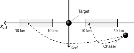
The control objective is to bring all relative non-singular orbital elements apart from∆θto zero. The variable∆θ
should instead be brought into one of two boxes. This is a non-convex constraint (Figure4). The side from which the
final approach is performed is determined byα(t) as described above.
xcrf
zcrf
Target
10 km
30 km −10 km −30 km
[image:15.595.181.415.243.335.2]Chaser
Figure 4: Choice of OSTG terminal set (not to scale)
Now, letting jN=t+NTs, the terminal constraint is a combination of
1 0 0 0 0 0
0 0 1 0 0 0
0 0 0 1 0 0
0 0 0 0 1 0
0 0 0 0 0 1
x(jN|t)= 0 0 0 0 0 (12)
(implemented as symmetric inequality constraints for compatibility with the available solver) and one of
0 1 0 0 0 0
0 −1 0 0 0 0
Σetgt(jN)
x(jN|t)≤
30×103
−10×103
(13) or
0 −1 0 0 0 0
0 1 0 0 0 0
Σetgt(jN)
x(jN|t)≤
30×103
−10×103
(14)
depending on the side from which the approach has been determined to occur, based on the angleα(t).
4.6. Tuning
The maximum prediction horizon during the OSTG phase must be long enough for the predicted open-loop
con-trolled trajectory to be feasible with respect to the terminal constraint and constraints imposed at other time steps
during the prediction horizon. The sampling periodTs and maximum prediction horizon Nmax must be chosen to
must be short enough to allow sufficient flexibility of control, but long enough that corrections due to navigation error
does not cause excessive propellant consumption. By performing batch simulations over a selection of different
pre-diction horizons, sampling times, and input weightings it was found thatNmax=25 andTs=600 s, withwu=10 was
a suitable compromise, leading to a total prediction horizon of 15000 s or approximately 1.5 orbits for the elliptical
scenario and 2 orbits for the circular scenario.
5. Short Range (INTG)
Once the OSTG MPC submodule has brought the chaser craft into the same orbit as the target, the separation
between them is still in the range of 10 km–30 km (Figure4) due to a difference in true anomaly between the two
vehicles. The INTG MPC submodule has the task of reducing this by performing a series of (passively safe) impulsive
transfers between a sequence of pre-specified holding points up until a point 100 m from the target.
Minimisation of propellant consumption is still critical, so variable horizon MPC with a 1-norm cost function is
considered for this phase also. Because it is unknowna priori when the flag permitting exit from a holding point will be raised, there is no point designing an MPC that predicts past the next holding point in the sequence. Whilst
there is not a strict prescription on the shape of the trajectories between holding points, there is an expectation that in
the absence of uncertainties these trajectories should resemble the conventional “bang-off-bang” hopping trajectories
(Fehse,2003), each lasting approximately half an orbit. For a given prediction horizon N, this allows a shorter sampling periodTsto be used than for the OSTG phase whilst maintaining an optimisation problem of similar size.
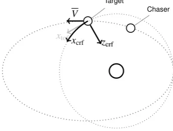
5.1. Holding Point Schedule
Holding points are periodic free-drift trajectories centred on a point a fixed distance away from the target. Because
it is unknown how long the chaser will be required to stay at any particular hold point, the MPC controller is designed
with the goal of reaching the “next” hold-point, with the position of the next hold-point provided to the MPC controller
as an input parameter. It is not guaranteed that the OSTG MPC controller will deliver the chaser to exactly the first
holding-point (in fact, from the perspective of fuel consumption and completion time, it is preferable for the chaser
to be delivered into the same orbit as the target with a reduced in-track separation). In such cases the first
hold-point is chosen as the closest hold-hold-point in the direction of the target from the chaser at the instant that the INTG
MPC controller is enabled (Figure5). Letxhpdenote the distance (in kilometres) from the target to the centre of the
currently scheduled holding point.
5.2. Prediction Model
For the short range (INTG) phase the Yamanaka-Ankersen (Yamanaka & Ankersen,2002) STM (state transition
xcrf
zcrf Target
[image:17.595.183.416.111.197.2]Chaser Varying∆νhold-point
Figure 5: Choosing the first hold point (example in elliptical orbit)
and velocities in a cylindrical reference frame (CRF) and is a generalisation of the classical Hill-Clohessy-Wiltshire
STM (Kaplan,1976;Sidi,1997;Fehse,2003) to elliptical orbits. The state vector is
x=
xcrf ycrf zcrf x˙crf y˙crf z˙crf
T
. (15)
The cylindrical co-ordinate frame (CRF) is a reference frame with its origin centred on the target (Figure6). Value
zcrfis the relative position in the radial direction (positive values towards the focus of the orbit), ycrf is the relative
position in the direction normal to the plane of the orbit, andxcrf is in the direction that completes the right-hand
set. The direction labelledV in Figure6corresponds to the instantaneous direction of the velocity of the target. It should be noted that this direction is time-varying with respect to the CRF for elliptical orbits, and aligned withxcrffor
circular orbits. The cylindrical reference frame is used in preference to a Cartesian target orbital frame (TOF) because
Target
Chaser
ztof
zcrf
xtofx
crf
V
Figure 6: Cylindrical reference frame (CRF)
it allows for relatively large in-track separations to be possible whilst keeping the linearisation error of a model of
relative dynamics model small. Linearisations from radial and out-of-plane separations are larger (Kaplan,1976;Sidi,
1997;Melton,2000), but nevertheless not significant over the ranges considered during the INTG phase.
The Yamanaka-Ankersen STM is linear parameter varying (LPV) in terms of the true anomaly of the targetνtgt.
However, because in this scenario the target is passive, under the assumption of perfect conditions, the target mean
anomaly can be propagated as a function of time. The propagated true anomaly can be recovered from the
[image:17.595.209.381.432.562.2]Kepler’s equation iteratively using Newton’s method (Sidi,1997). This allows the Yamanaka-Ankersen STM to be
implemented as an LTV model.
For the INTG phase, an impulsive discretisation is used to best represent the nature of the input trajectory expected,
and scaling is performed so thatxcrf,ycrfandzcrfare measured in kilometres, the velocities in the CRF are expressed
in metres per second, and that the “input” is an impulsive∆V is expressed in units of 0.1 ms−1. The scaling is to
improve numerical stability by ensuring that all decision variables and constraints are of similar magnitude. IfΦ(t) is the unmodified Yamanaka-Ankersen STM with states expressed in m and ms−1then matrixA(t) is calculated as
A(t)=diag
10−3
10−3
10−3
1 1 1
Φ(t)diag
103 103 103 1 1 1 (16)
andB(t) is calculated as
B(t)=A(t)
03×3
0.1I3×3
. (17)
5.3. Variable Horizon Cost Function
Like for OSTG, in order to ensure finite time completion whilst minimising propellant consumption, a 1-norm
cost function is used in conjunction with a variable horizon, however unlike OSTG, INTG does not apply a weighting
on planned time to finishi.e.the horizon N. Instead, a weighting on distance is employed, as it provides a more consistent response over the range of distances that INTG has to handle. A fixed tuning of time weight would provide
overly aggressive control at short distances. Letting j=t+kTs, the cost function to be minimised is chosen to be:
J= N−1
X
k=1
kEc(xcrf(j|t)−r(j))k1+wuku(j|t)k1
.
(18)
wherewuis the weighting on input (∆V) relative to distance, andEcis a weighting matrix selecting the out-of-plane
and in-track components of the state vector:
Ec=
0 1 0 0 0 0
0 0 1 0 0 0
. (19)
The referencer(j) is chosen as
r(j)=
−xhp(1+ecosν(j)) if approach fromx<0
xhp(1+ecosν(j)) if approach fromx>0.
(20)
The reference trajectory traces thexcrfposition of avarying-∆νholding point at distancexhpon the appropriate side
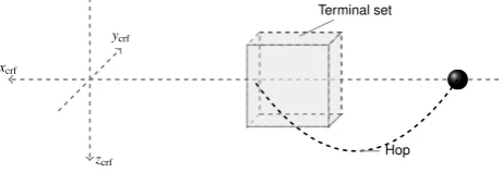
5.4. Terminal Constraints
The terminal constraint can be split into five components. The constraint on the immediate position in the terminal
constraint is given as:
I 0
−I 0
x(jN)≤chp(jN). (21)
This constrains the position of the chaser at time jN =t+NTsto be inside a box, centred on a pointxhpaway from
the target onV, of width 2xhpe+ in the orbital plane and 0.6xhpe+ in the out-of-plane direction (Figure 7), where
e+ =etgt+0.1 to ensure that the box is non-empty for a circular orbit. The rationale for this constraint is that it is
sufficient to contain avarying∆νperiodic trajectory, whilst limiting out-of-plane motion without driving it completely to zero. Similar constraints can be given for the position after 1/4, 1/2 and 3/4 orbits. The constraints on the position
xcrf
zcrf ycrf
Terminal set
[image:19.595.184.415.300.379.2]Hop
Figure 7: INTG terminal set (>5 km)
1/4, 1/2 and 3/4 orbits aftert+NTsare given as:
I 0
−I 0
A(jN;jN+ ∆T)x(jN)≤chp(jN+ ∆T),
∀∆T ∈ {T1/4,T1/2,T3/4}. (22)
Finally, in order that the holding point can be periodic, an invariance condition must be imposed. Due to the relative
dynamic model only having one non-periodic mode, it is sufficient to only impose this constraint on thexcrfstate:
1 0 0 0 0 0
(A(jN;jN+Torb)−I)x(jN)=0. (23)
The MPC controller for INTG is used to provide combined guidance and control. Because a variable horizon is
being used, the control objective must be encoded in the choice of terminal set. As described previously, the objective
of the INTG MPC controller is to impulsively transfer the chaser from one holding point to the next. When the holding
point is at a distance further than 5 km, the INTG MPC controller is designed with a terminal constraint that the chaser
be on a periodic trajectory that is inside a box centred on the hold-point position onV-bar in the cylindrical reference frame after free-drift periods of 1/4, 1/2 and 3/4 orbits in terms of true anomaly (with corresponding times denoted as
prediction horizon for 1/4, 1/2 and 3/4 orbits.
ν(jN+T1/4)=ν(jN)+π/2 ν(jN+T1/2)=ν(jN)+π/4 ν(jN+T3/4)=ν(jN)+3π/2
The mean anomalyM(t) is obtained from the true anomalyν(t) using the equation (Sidi,1997):
M(t)=2 tan−1
√
1−etan(ν/2) e√1−e2− √1+esinν
1+ecosν
. (24)
Noting thatM(t)=n∆t, where∆tis defined to be the time since the target last passed the periapsis of its orbit, andn is the mean anomaly rate (Sidi,1997), the times for 1/4, 1/2 and 3/4 orbits can be calculated as:
T1/4= (∆t(jN+T1/4)−∆t(jN)) modTorb (25a)
T1/2= (∆t(jN+T1/2)−∆t(jN)) modTorb (25b)
T3/4= (∆t(jN+T3/4)−∆t(jN)) modTorb. (25c)
Remembering that xhpis the absolute holding point distance from the target (in kilometers), ande+ =etgt+0.1,
then define vector
chp(t)=
−xhp(1−e+)
0.3xhpe+
xhpe+
xhp(1+e+)
0.3xhpe+
xhpe+
| {z }
xcrf(t)<0
or
xhp(1+e+)
0.3xhpe+
xhpe+
−xhp(1−e+)
0.3xhpe+
xhpe+
| {z }
xcrf(t)>0
(26)
which is used in (22).
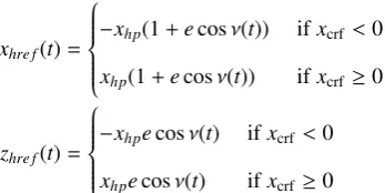
5.5. Terminal Constraints (Hopping<5 km)
If the next hold point is equal to, or closer than 5 km, the terminal constraint is stricter. Instead of requiring the
chaser to be on an arbitrary periodic trajectory that remains within a fixed box in the cylindrical reference frame, the
terminal constraint requires that the chaser enters a trajectory in proximity to avarying∆νholding trajectory. This is so that at the final holding point (the TAP), there is little overshoot when switching to the FTTG mode which regulates
toV. Constraints (21) to (22) are modified by changingchp(t) to be:
chp(t)=
xhre f(t)+|δxhre f|
0.3xhpe+zhre f(t)+|δzhre f|
−xhre f(t)+|δxhre f|
where
xhre f(t)=
−xhp(1+ecosν(t)) ifxcrf<0
xhp(1+ecosν(t)) ifxcrf≥0
(28a)
zhre f(t)=
−xhpecosν(t) ifxcrf<0
xhpecosν(t) ifxcrf≥0
(28b)
andδxhre f andδzhre f are tolerances based upon an upper bound on the largest propagation of the expected worst-case
sensor uncertainty through the prediction model
δxhre f
δyhre f
δzhre f
=A+(j;j+Ts)wmax
wherewmaxis a vector consisting of the element-wise maximum absolute navigation errors andA+(t) is a matrix whose
elements are the absolute values of the elements ofA(t), defined as:
A+,nA+∈R6×6|A+i j=|Ai j|,∀i∈ {1, . . . ,6}, j∈ {1, . . . ,6} o
. (29)
Terminal set
xcrf
zcrf ycrf
[image:21.595.211.385.130.217.2]Hop
Figure 8: INTG terminal set (<5 km)
5.6. Input Constraints
Nominal input constraints are imposed in exactly the same way as for OSTG, except they are imposed with respect
to the cylindrical reference frame (CRF) rather than the chaser orbital frame (COF).
5.7. Short-Term Passive Safety
Passive safety is considered in a similar manner as OSTG, with free drift propagations made for a whole orbit from
each open-loop controlled prediction (7). Because the Yamanaka-Ankersen equations directly propagate the relative
position dynamics in the CRF, the geometric transformationΣis not required, and the safety constraint is:
−sgn(xcrf(t)) 0 0 0 0 0
xfree(j+iTsafe|j|t)≤ −RS t)
Unlike during the OSTG phase, the angleαof the halfspace approximation to the safety sphere may only take on
values 0 andπ. This is because during the INTG phase the expected trajectory should never pass over or underneath
the target because in a capture scenario, the final approach can be performed from either direction.
5.8. Long-Term Passive Safety
In addition to ensuring that no passive drift trajectory intersects the safety sphere during the period of one orbit, an
extra requirement is imposed at ranges<5 km to ensure that the passive drift trajectory does not intersect the safety
sphere within 10 orbits. Rather than explicitly predicting the full 10 orbits, a drift condition is imposed to ensure that
after a single orbit, the chaser is at least as far away from the target as it is currently. This is expressed as
−sgn(xcrf(t)) 0 0 0 0 0
(A(j;j+Torb)−I)x(j)≤0 (31)
where in this case,j=t+kTs ∀k∈ {1, . . . , N−1}. By doing this, a free drift trajectory will always (on average) move
away from the target. Thus, as long as no collision occurs during the first complete orbit of passive drift (enforced by
the short-term passive safety constraints), no collision will occur during subsequent orbits.
5.9. Constraint Tightening
In order to account for navigation uncertainty, each of the running constraints are subsequently tightened using the
nilpotent disturbance feedback policy proposed in (Richards & How,2003b,a), adapted to the LTV system dynamics.
It is assumed that most uncertainty comes from navigation error, therefore, the worst-case uncertainty is assumed to
be within the 3σvalues shown in Table3 when closer than 5 km. To avoid infeasibility, at greater than 5 km the
constraint tightening is relaxed to consider only 1σnoise values. Qualitatively, the effect of this is to make the passive
safety constraints more conservative, and the drift condition equal to a predicted passive drift away from the target
rather than merely not drifting towards the target. To avoid infeasibility, the terminal constraint is not tightened.
5.10. Tuning
The maximum prediction horizon during the INTG phase must be sufficient to feasibly encompass a complete
transfer from one holding point to the next. In a circular orbit, a single impulsive radial or tangential “hopping”
manœuvre (Fehse,2003) takes exactly half an orbit. In an elliptical orbit there is a small amount of variability
dependent on the target true anomaly. As for the OSTG phase,Tsshould be short enough to allow impulsive thruster
burns at the optimum times, but long enough that excessive decision variables are not required in the optimisation,
and that propellant consumption is not dominated by corrective manœuvres caused by navigation uncertainty. By
performing batch simulations over a selection ofTsandwu, it was found that a setting ofTs =300 s was suitable,
alongside an input weightingwu =0.2. WithNmax =20, this corresponds to 6000 s, or 0.8 orbits for the circular
6. Terminal to Capture (FTTG)
The objective of the final translation phase (FTTG) is to control the chaser along a straight-line trajectory a few
centimetres fromVtowards the target. The FTTG phase ends at a point, approximately 3 m from the target, where the LIDAR view is blocked by parts of the chaser spacecraft itself. At this point, all control authority is relinquished,
and the final capture occurs during a passive drift trajectory. If, due to a fault, or higher than expected navigation
error the chaser arrives in the neighbourhood of the target at a higher velocity than expected, or on a trajectory that
cannot be corrected in time, a collision avoidance manœuvre (CAM) must be commanded. During the FTTG phase,
attitude control is performed using the thrusters rather than reaction wheels, and is included in the remit of the MPC
controller. The MPC must maintain LIDAR target pointing in order to preserve relative navigation.
6.1. Thruster-Aligned Prediction Model
During the FTTG phase, attitude control is performed using thrusters rather than reaction wheels, and becomes
part of the responsibility of the MPC controller. Due to the thruster geometry, there is cross-coupling between the
inputs to the translational dynamics and the attitude dynamics (each thruster input provides a non-zero torque in
combination with a force). This can be represented mathematically as
δxtr(j+Ts) δxat(j+Ts) =
Atr(j) 0
0 Aat(j)
δxtr(j)
δxat(j)
+
Btr(j) 0
0 Bat(j)
Mtr Mat
u(j)+ 0
fat(j)
+
dtr(j)
dat(j)
(32)
whereδxtr(j) andδxat(j) are the state differences from the linearisation point at timej,u(j)∈R8is a vector of thruster
commands at time j,Mtr ∈R3×8is a matrix whose columns comprise the unit vector force directions of each of the
thrusters in the CRF, andMat ∈ R3×8is a matrix whose columns comprise the unit vector torque directions of each
of the thrusters in the chaser reference frame. The bias fat(j) arises from the linearisation of the attitude around a
non-equilibrium setpoint. The biasesdat(j) anddtr(j) arise from addition of a state disturbance estimate for offset-free
control.
6.2. Trajectory Prediction Model
For the FTTG phase trajectory control, the LTV Yamanaka-Ankersen STM is also used, but with a shorter sampling
period. Instead of an impulsive discretisation, a pulse discretisation is used, whereby a pulse of thrust is allowed for
δTs in every period of length Ts. It was found that a conventional zero-order hold discretisation did not improve
accuracy. This was due to navigation errors. However, it was found that constantly commanding continuous
low-level thrusts led to differential thrust being used to achieve the commanded forces, and thus excessive propellant
consumption. The differential thrust occurs to counteract the effects of the minimum impulse bit (MIB). The MIB
that described in (16), albeit discretised at a different rate, but theBtr(t) matrix is approximated by discretising the
instantaneous nonlinear continuous dynamics,
Btr(t)=Atr(t+δTs;t+Ts)M12 (33)
where
M11 M12
0 I
=exp
Atr,c(t) Btr,c(t)
0 0
δTs
(34)
andAtr,c(t) is the instantanous linearised realisation of the continuous time state-space relative dynamics (described in
Yamanaka & Ankersen(2002)) andBtr,c(t)=m−1
03×3 I3×3
T
corresponds to a force input (wheremis the mass of the chaser in kilograms). The notationA(t+δTs;t+Ts) denotes the open-loop unforced STM from timet+δTs to
timet+Ts.
6.3. Attitude Prediction Model
Whilst attitude control is not considered in the MPC design for the OSTG and INTG phases (during these phases
it is assumed that target-pointing is handled independently using momentum wheels), during the very short range
FTTG phase, the MPC is responsible for attitude control as well as trajectory control. A small-angle quaternion-based
attitude dynamics model is used. This is similar to that used by (Hegrenæs et al.,2005), however, because an elliptical
orbit must be considered, this must also be implemented as an LTV model, and must account for the rate of rotation
between the velocity orbital frame (VOF) and the inertial frame.
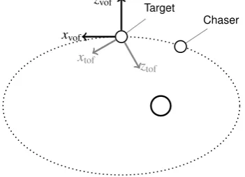
Like the cylindrical reference frame, the velocity orbital frame (VOF) has its origin placed at the target centre
of mass. However, the directionxvof is aligned withV. The direction yvof is aligned with the direction of angular
velocity of the orbit, andzvofcompletes the right-hand set (Figure9). The alignment ofxvofis advantageous when a
Vapproach is performed in an elliptical orbit as the attitude setpoint will remain approximately constant with respect to this reference frame. Using this reference frame is advantageous when performing the final straight-line approach
Target
Chaser
ztof xtof
xvof
[image:24.595.208.384.549.676.2]zvof
Figure 9: Velocity orbital frame (VOF)
pointing during this phase for the same reason. To avoid discontinuities in the attitude quaternion when approaching
from “in front” of the target, a reference frame based on the VOF but rotated byπabout thezvof axis can be used
(Bach & Paielli,1993).
The attitude kinematics can be described using the nonlinear continuous-time model derived from Euler’s moment
equations
d dt ω
c vc
c=I
−1 chsN−I−
1 chs
ωc
iv+ω c vc
×Ichs
ωc
iv+ω c vc
−ω˙civ+(ωcvc×ωciv) (35)
whilst the attitude dynamics can be described using the model
˙ η ˙ ǫ = 1 2
−ǫTωc vc
ηωc
vc+(ǫ×ωcvc) (36)
whereωcvcis the angular velocity between the chaser and the VOF, ωcivis the angular velocity between the inertial
frame and the VOF,
η ǫT
T
is a quaternion representation (e.g. Wertz(1978)) of the rotation between chaser and
VOF andIchsis the matrix representation of the moment of inertia of the chaser. These can be combined into a single
MIMO differential equation and, as the model must be time-varying to accommodate the elliptical orbit, there is little
extra effort required to re-linearise about the current attitude measurement at each sampling instant to obtain a linear
local state space model
δx˙at(t|t0)=Aat,c(t|t0)δxat(t|t0)+Bat,c(t|t0)N(t) (37)
where the index notation (t|t0) used here implies the prediction at timetlinearised about the measurements taken at
timet0, and the deviation from the linearisation point
δxat(t|t0)=
ωc vc(t) η(t)
ǫ(t)
− ωc vc(t0)
η(t0)
ǫ(t0)
. (38)
The linearised time-varying continuous time state space matrices are defined as:
Aat,c(t|t0)=∇
d dt(ω
c vc(t0))
c
˙
η(t0)
˙
ǫ(t0)
ωc
iv(t),ω˙civ(t)
(39)
and
Bat,c(t|t0)=
Ichs−1 0 . (40)
The instantaneous continuous time dynamics are then discretised using the sameδTsin everyTspulse discretisation
used for the trajectory model to obtain a discrete time model