promoting access to White Rose research papers
White Rose Research Online
[email protected]
Universities of Leeds, Sheffield and York
http://eprints.whiterose.ac.uk/
This is a copy of the final published version of a paper published via gold open access
in
Annales Geophysicae
.
This open access article is distributed under the terms of the Creative Commons
Attribution Licence (
http://creativecommons.org/licenses/by/3.0
), which permits
unrestricted use, distribution, and reproduction in any medium, provided the
original work is properly cited.
White Rose Research Online URL for this paper:
http://eprints.whiterose.ac.uk/78604
Published paper
www.ann-geophys.net/31/1611/2013/ doi:10.5194/angeo-31-1611-2013
© Author(s) 2013. CC Attribution 3.0 License.
Annales
Geophysicae
Determination of wave vectors using the phase differencing method
S. N. Walker1and I. Moiseenko2
1Department of Automatic Control and Systems Engineering, University of Sheffield, Sheffield, UK
2Space Research Institute of the Russian Academy of Sciences, Moscow, Russia
Correspondence to: S. Walker ([email protected])
Received: 25 February 2013 – Revised: 29 May 2013 – Accepted: 17 August 2013 – Published: 27 September 2013
Abstract. Due to the collisionless nature of space plasmas,
plasma waves play an important role in the redistribution of energy between the various particle populations in many re-gions of geospace. In order to fully comprehend such mech-anisms it is necessary to characterise the nature of the waves present. This involves the determination of properties such as wave vectork. There are a number of methods used to cal-culatekbased on the multipoint measurements that are now available. These methods rely on the fact that the same wave packet is simultaneously observed at two or more locations whose separation is small in comparison to the correlation length of the wave packet. This limitation restricts the analy-sis to low frequency (MHD) waves. In this paper we propose an extension to the phase differencing method to enable the correlation of measurements that were not made simultane-ously but differ temporally by a number of wave periods. The method is illustrated using measurements of magnetosonic waves from the Cluster STAFF search coil magnetometer. It is shown that it is possible to identify wave packets whose coherence length is much less than the separation between the measurement locations. The resulting dispersion is found to agree with theoretical results.
Keywords. Space Plasma Physics (Experimental and
math-ematical techniques; Wave-particle interactions; Waves and instabilities)
1 Introduction
The collisionless nature of space plasma means that plasma waves and turbulence play an integral role in the interactions between the various particle populations that exist within the plasma. They form the path by which energy may be ex-changed between the ion species and also electrons. Thus, in order to understand these processes it is necessary to identify
the various wave modes that exist within the plasma and also determine their characteristics. One key parameter to deter-mine is the wave vectork. The vector direction is the direc-tion of propagadirec-tion of the wave whilst its magnitude defines its wave number (k) and is related to the wavelength (λ)by
k=2π/λ. Knowledge of the wave vector is often a crucial parameter that is required within theoretical descriptions of wave-particle interactions. For instance, theoretical studies of ElectroMagnetic Ion Cyclotron (EMIC) waves in the in-ner magnetosphere have shown that the EMIC waves may accelerate ions whose energy is proportional to the k vec-tor (Pakhotin et al., 2013), lower hybrid waves may transfer energy between electrons and ions whose Larmor radii are of similar size to the components of thekvector in the di-rection parallel and perpendicular to the local magnetic field (e.g. Walker et al., 2008), whilst statistical properties of cho-rus emissions may be used to probe density irregularities along the wave path (Agapitov et al., 2010, 2011). Within the radiation belts, magnetosonic waves form an integral part of the mechanism to accelerate electrons to very high ener-gies (Friedel et al., 2002; Horne et al., 2007). However, it is still unclear which external influence modulate the gen-eration mechanism of these electrons (Reeves et al., 2011; Balikhin et al., 2011; Boynton et al., 2011).
1612 S. N. Walker and I. Moiseenko:kvector determination
Pinçon and Glassmeier, 2008). For instance, thek filtering technique requires at least four point vector measurements and a longer time series whilst the phase differencing tech-nique may be applied to scalar values and requires shorter intervals of data. However, thekfiltering technique can suc-cessfully identify waves when more than one mode is present at a particular frequency. The two limitations of simultane-ous observations and that the coherence length of the wave is larger than the separation of the measurement locations essentially restrict the applicability of such analyses to low frequency (MHD) waves. This paper discusses an extension to the phase differencing method to the identification of wave packets that are observed at separations much larger than the coherence length of the individual wave packets. Section 2 outlines the basic method used to determine the wave vec-tor for cases when two point and multi-point (at least four) measurements are available. An extension to this method is described in Sect. 3 which enables the correlation of wave packets whose observations at different locations are tempo-rally separated by a large number of wave periods. An exam-ple of the use of this method is shown in Sect. 4 based on the observation of packets of magnetosonic waves. Section 5 compares the experimentally determined wave vector to the theoretical dispersion curve and the results are summarised in Sect. 6.
2 Phase differencing
The phase differencing method assumes that in the plasma rest frame the wave field can be represented as the superpo-sition of a number of plane waves.
B(r, t )=6ωBωexp[i(k·r−ωt )] +cc (1)
where Bωis the wave amplitude at frequencyω,kis the wave vector (kvector),r is the separation vector between the lo-cation of the two (or more) simultaneous measurements, and cc represents the complex conjugate term. If the same wave is measured by two closely spaced satellites, then there will be a phase shift1ψin one signal relative to the other. The magnitude of the phase shift is related to the component of the wave vectorkr projected along the separation directionr between the two measurement points by
1ψ (ω)=k(ω)·r+2nπ
= kkkkrkcos(θkr)+2nπ (2)
whereθkr is the angle between the wave vector k and the satellite separation vectorr. The factor 2nπ arises from the fact that the method will only determine the phase difference within the range−2π < 1ψ <2π and so result in a peri-odic family of solutions. Thus, it is important to ascertain the value ofnin order to determine the actual projection of the
kvector along the satellite separation vector (kr) correctly. This is usually accomplished by inspection and comparison
of the two waveforms. This point will be discussed more in the later sections of this paper.
The result of this analysis is a dispersion curve that shows a histogram of the measured amplitudes that occurred in the data period analysed as a function of the wave frequency and phase difference between the two measurements. From such a plot it is then straight forward to determine values ofkras a function of frequency (Balikhin et al., 1997b; Chisham et al., 1999; Balikhin et al., 2001).
If data are measured at four (or more), non-coplanar points it is possible to reconstruct the complete k vector directly from its componentskralong three independent satellite sep-aration directions (Balikhin et al., 2003). In this case,
k=R·kr (3)
where R is a matrix whose columns are the normalised sepa-ration vectors (Bates et al., 2000).
However, if such simultaneous datasets are unavailable it is still possible to reconstruct the full k vector if another method, such as variance analysis, may be used to determine its direction. This assumes that the wave is electromagnetic in nature, not linearly polarised, and that the analysis is ap-plied to measurements of the magnetic field. In this case, the direction of propagation is defined by the minimum variance direction. It should be noted that there is an ambiguity of 180◦ in the direction of the minimum variance component. Its actual direction may be determined by comparing the two waveforms to see the order in which the spacecraft observed the wave and therefore deduce the constraint that this places in the propagation direction of the wave. Thus, the full k
vector may be resolved using the direction determined from the variance analysis and its component measured along the satellite separation vector (Balikhin et al., 1997a).
3 Determination ofn
As mentioned above, one of the key aspects to calculating thekvector using the phase differencing technique is to de-termine the value ofn that appears in the phase ambiguity factor 2nπthat appears in Eq. (2). In some cases, the value of
nis obvious. Examples include the analysis of isolated wave packets that exist with no other wave activity occurring in the immediate vicinity. A good example of this was reported by Balikhin et al. (2005) who used this technique to identify the occurrence of ion sound waves in the foot of the quasiper-pendicular shock front. In this case, the two waveforms could easily be matched andndetermined. In such cases,nwould be expected to take a small value, sayknk<5. For low fre-quency waves, whose wavelength is larger than intersatel-lite separation distance, the value ofnwill be zero and also
1ψmay be determined directly from the waveforms. In such cases, the branch of the dispersion curve passes through the origin (kr =0, ω=0) so thatn=0.
This then naturally invites the question regarding the pos-sibility of determiningnif the separation between measure-ment locations is large when compared to the wavelength of the waves. In such cases, the second satellite may observe the wave packet either at a separation distance corresponding to many wavelengths from the first satellite or after a time pe-riod that corresponds to many wave pepe-riods has elapsed as-suming the satellite separation vector has a large angle to the
kvector. So, how is it possible to determine the value ofn
in these cases? The key to answering this question is to ex-amine the overall shape or envelope of the wave packet(s). Observations of the same wave packet at locations separated by a few 10’s of wavelengths would be expected to exhibit similar structure provided the wave has not evolved a signifi-cant amount as it propagated through the intervening plasma. For an isolated wave packet it is straight forward to compare the two waveforms to establish that the measurement are of the same wave packet and then determine the time differ-ence between similar features in the wave packet measured at different locations. Once the frequency of the wave packet is known, the value ofncan be calculated easily. However, if a continuous series of wave packets are observed this be-comes more problematic. Thus, in this paper an extension to the phase differencing technique, based upon the envelope of the waveform, is employed to determine the offset between the two datasets. There are a number of procedures that may be adopted to calculate the envelope of a waveform, typi-cally taking the real waveform, reconstruct the complex part that is lost and then calculate the complex modulus or mag-nitude of the data. In this paper we use a method based upon wavelet transforms as opposed to the Hilbert transform. It should be noted, however, that both methods produced very similar results.
4 Example
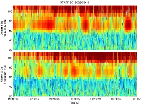
The data used to illustrate this method were collected by the Cluster STAFF search coil magnetometer instruments (Cornilleau-Wehrlin et al., 1997) onboard spacecraft 1 and 2 on 13 March 2002 between 16:40 and 17:15 UTC. During this period, the Cluster satellites were situated in the inner magnetosphere at a geocentric distance of around 4.4REon the night side (local time∼00:50) and a magnetic latitude of≈3◦ above the magnetic equator at the beginning of the period and moving in a northerly direction. Between 16:42 and 16:52 all Cluster satellites observed a general increase in wave activity in the frequency range 90–150 Hz. Examina-tion of the STAFF propagaExamina-tion parameters (CAA data prod-uct not shown) reveal that these waves are typically propa-gating perpendicular to the external magnetic field and pos-sess a high degree of ellipticity. These properties are typical of magnetosonic waves. It is also noticeable that the most intense emissions also exhibit a banded structure in the fre-quency range from≈70 Hz up to≈170 Hz, i.e. they are
ob-Fig. 1. Wavelet spectra of the magnetic fieldBZcomponent mea-sured by STAFF-SC onboard Cluster 1 (top) and Cluster 2 (bottom) showing a band of emissions centred around 70 Hz.
served over a greater frequency range than the magnetosonic waves, similar to those reported by Russell et al. (1970) and Gurnett (1976). The background magnetic field was deter-mined using data from the FGM instrument Balogh et al. (1997). Unfortunately, a data gap exists in the period of in-terest and so the background magnetic field vector was de-termined by smoothing the data using a one minute sliding window and then interpolating across the gap. This method appeared to produce more realistic result than those obtained from a model field. The actual difference in the total mag-netic field resulting from the two methods was around 3 %. The field vector used in the subsequent analysis was (20, 137, 308) nT (magnitude 338 nT) in the GSE frame which re-sults in a proton gyrofrequency around 5.2 Hz and an electron gyrofrequency of 9.5 kHz.
[image:4.595.309.544.61.234.2]1614 S. N. Walker and I. Moiseenko:kvector determination
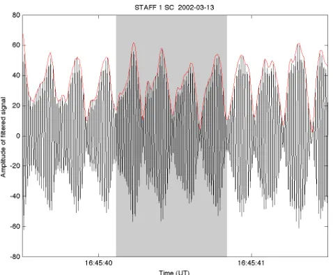
Fig. 2. Structure of wave packets observed by Cluster 1 on
13 March 2002 between 16:45:39.5 and 16:45:41.5 UTC.
h(t )= 1
π1/4exp(−2π it )exp(−t
2/2) (4)
The resulting filtered waveform is complex in nature. The amplitude profile, or envelope, of these packets may then be calculated using the complex modulus of the filtered data. An example of the waveform and its packet structure is shown in Fig. 2. The black line is the 70 Hz filteredBZ waveform measured by STAFF-SC on spacecraft 1. It clearly shows the packet nature of the emissions. The red line shows the outline packet structure (modulus of the complex data). This clearly shows the fact that every packet has a slightly differ-ent shaped envelope depending upon the phases of the beat frequencies. Thus, in order to determine the phase offsetn
between the two measurement locations a comparison is re-quired based on the packet structures of the two measure-ments. The grey region of Fig. 2 highlights four consecutive wave packets whose envelope shapes are quite distinctive. These packets form the basis for the comparison between the two datasets.
Figure 3 shows the shape of the packet envelopes for Clus-ter 1 (black) and ClusClus-ter 2 (red). In the top panel both quan-tities are plotted against their own time tags. There is no clear correlation between the structures of the wave pack-ets shown in this panel. They are completely different. How-ever, on closer inspection it is clearly seen that some of the wave packets observed by Cluster 1 bear a striking resem-blance to packets observed by Cluster 2 around 0.6 s later. A cross correlation analysis was performed using the enve-lope data to determine an approximate time offset. The exact time offset was then calculated based on the waveforms of the packets under study. The lower panel of Fig. 3 compares the packet structures after a timing offset of−604 ms has
Fig. 3. Structure of wave packets observed by Cluster 1 (black)
and Cluster 2 (red) on 13 March 2002 between 16:45:39.5 and 16:45:41.5 UTC. In the top panel the two series are shown with their original time tags. In the lower panel, the Cluster 2 data has been shifted by 604 ms to align it with the Cluster 1 measurements.
been applied to Cluster 2 (the time axis refers to Cluster 1). In this case there is a very good correlation between the two datasets with many of the features observed by Cluster 1 also observed in the Cluster 2 data. Thus, it appears as if Cluster 2 sees the same wave packets as Cluster 1 with a time delay of around 600 ms. This corresponds to around 42 periods of a wave with frequency 70 Hz.
To determine the exact delay the waveforms of the pack-ets in question should be compared. By adjusting the timing offset applied to the Cluster 2 data it was found that the ex-act time difference between the two datasets was−604 ms, which corresponds to−42.28 wave periods. Figure 4 com-pares the waveforms of the packets highlighted in Fig. 2 as observed by Cluster 1 (black) and Cluster 2 (red) 604 ms later. It is clear that these are indeed the same wave packets measured by the two satellites.
Using a time offset of−600 ms (which corresponds to 42 periods of a 70 Hz wave) for the Cluster 2 data the ω−k
dispersion was computed using the phase differencing tech-nique. From the analysis presented above it was determined that the exact time offset was 604 ms which corresponds to 42.28 wave periods. Therefore, the results of the phase differ-encing calculations should show a peak at around−1.75 rads at a frequency of 70 Hz. The results of the analysis, shown in Fig. 5, do indeed show a peak at this location inω−k
space. Further examination of Fig. 4 shows that whilst the maximal amplitudes of the wave packets coincide, the min-ima between the packets may show a phase variation of up toπ/2. This effect will make the dispersion branches shown in Fig. 5 to widen and hence result is slightly larger errors. However, the main result would be unaffected.
[image:5.595.310.543.62.248.2]Fig. 4. A comparison of two wave packets measured by Cluster 1
and Cluster 2 with a time offset of 604 ms.
For this example, the direction of thekvector was deter-mined from the STAFF spectral matrix data available from CAA. In science burst mode, this dataset provides the full spectral matrix for 18 frequencies in the range 70 Hz–4 kHz at a time resolution of 1 s. Thus, the resulting direction will be the average of all wave activity during this period. The wave vector direction was calculated based on the values of the spectral matrix using the methods of McPherron et al. (1972) and Santolik et al. (2003) to be (0.12,−0.99, 0.002). This direction lies almost perpendicular to the background magnetic field (θBk=83◦). However, it should be noted that the ratio of the intermediate to lowest eigenvalue determined during this calculation was in the range 2–3, which implies that the minimum variance direction is not resolved partic-ularly accurately. The error in direction, estimated using the method of Hoppe et al. (1981) is>20◦. This represents the
major source of error in the following calculations. Never the less, these values will be used for the example calculation.
Since the measured value ofkr represents the projection of thekvector onto the satellite separation direction the full
kvector may be reconstructed using Eq. (3). From the calcu-lations above, the observed phase difference is 42.28×2×π
rad. The separation vector between satellites 1 and 2 was (12.8,−40.0,−182.6) km (GSE) and thusθkr= 64◦. Thus, the magnitude of the wave vectork∼0.3 km−1.
5 Comparison with theory
[image:6.595.48.285.63.248.2]Magnetosonic waves are electromagnetic emissions that are often observed within 3◦ of the magnetic equator, between 2≤L≤7, and 10–22 MLT. They occur in the frequency band between the proton gyrofrequency and the lower hy-brid resonance frequency and are thought to be generated by instabilities associated with a ring distribution of energetic
Fig. 5. Theω−kdispersion function calculated using Cluster 2 data with a time offset of 600 ms.
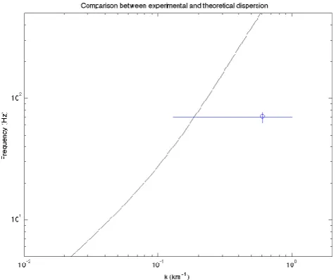
Fig. 6. Comparison of experimental and theoretical results.
protons of the order of 10 keV (Horne et al., 2007; Chen and Thorne, 2012). The waves themselves propagate at angles ap-proximately perpendicular to the magnetic field (θBk∼89◦) and are elliptically polarised with an ellipticity of≈0. The dispersion relation, derived using the cold plasma approx-imation and assuming that ω2pe2e and 2i ω2e, where ωpe2 is the electron plasma frequency and 2e(i) is the electron (ion) cyclotron frequency, may be written as (Musher and Sturman, 1975)
ω2 2 e
= k
2
k
1+k⊥2
+ω
2 LH
2 e
!
k2
1+k2 (5)
[image:6.595.309.548.292.491.2]1616 S. N. Walker and I. Moiseenko:kvector determination
electron inertial length. Figure 6 shows a section of the magnetosonic dispersion curve calculated using Eq. (5). The magnitude of thekvector determined above, represented by the circle, lies close to this curve, indicating that the wave type analysed is most probably a magnetosonic mode. As noted above, the major source of errors in the determination ofkis related to the inaccuracies in the determination of the minimum variance direction.
6 Summary
This paper has discussed a method to establish the phase difference between wave packets that are observed by two spacecraft at times separated by a large number of wave pe-riods. The key is to match the two wave packets in question by first analysing the shape of the wave packet envelopes to determine the approximate time difference between the two observations of the same wave packet. This step of the anal-ysis extends the usage of the phase differencing technique to wave packets that are observed at similar times, i.e. observed within a few wave periods in contrast to previous studies that were restricted to simultaneous observations. This method was then applied to the identification of wave packets ob-served in the vicinity of the magnetic equator. It was shown that there wave are probably magnetosonic in nature since the experimentally determined value of thekkk lies extremely close to the magnetosonic branch of the dispersion relation.
Acknowledgements. The authors wish to thank the Cluster STAFF and FGM teams for making their data available through the Cluster Active Archive. This joint study was funded in the framework of a Royal Society International Collaboration grant. SNW is grateful to STFC for financial support.
Topical Editor M. Gedalin thanks two anonymous referees for their help in evaluating this paper.
References
Agapitov, O., Krasnoselskikh, V., Zaliznyak, Yu., Angelopoulos, V., Le Contel, O., and Rolland, G.: Chorus source region localiza-tion in the Earth’s outer magnetosphere using THEMIS mea-surements, Ann. Geophys., 28, 1377–1386, doi:10.5194/angeo-28-1377-2010, 2010.
Agapitov, O., Krasnoselskikh, V., Dudok de Wit, T., Khotyaintsev, Y., Pickett, J. S., Santolík, O., and Rolland, G.: Multispacecraft observations of chorus emissions as a tool for the plasma den-sity fluctuations remote sensing, J. Geophys. Res., 116, A09222, doi:10.1029/2011JA016540, 2011.
Balikhin, M. A. and Gedalin, M. E.: Comparative analysis of differ-ent methods for distinguishing temporal and spatial variations, in: Proc. of START Conf., Aussois, France, Vol. ESA WPP 047, 183–187, 1993.
Balikhin, M. A., Dudok de Witt, T., Woolliscroft, L. J. C., Walker, S. N., Alleyne, H., Krasnoselskikh, V., Mier-Jedrzejowicz,
W. A. C., and Baumjohann, W.: Experimental determina-tion of the dispersion of waves observed upstream of a quasi–perpendicular shock, Geophys. Res. Lett., 24, 787–790, doi:10.1029/97GL00671, 1997a.
Balikhin, M. A., Walker, S. N., Dudok de Witt, T., Alleyne, H. S., Woolliscroft, L. J. C., Mier-Jedrzejowicz, W. A. C., and Baumjo-hann, W.: Nonstationarity and Low Frequency Turbulence at a Quasi-perpendicular Shock Front, Adv. Sp. Res., 20, 729–734, doi:10.1016/S0273-1177(97)00463-8, 1997b.
Balikhin, M. A., Schwartz, S., Walker, S. N., Alleyne, H. S. C. K., Dunlop, M., and Lühr, H.: Dual-spacecraft observations of stand-ing waves in the magnetosheath, J. Geophys. Res., 106, 25395– 25408, doi:10.1029/2000JA900096, 2001.
Balikhin, M. A., Pokhotelov, O. A., Walker, S. N., Amata, E., An-dre, M., Dunlop, M., and Alleyne, H. S. K.: Minimum vari-ance free wave identification: Application to Cluster electric field data in the magnetosheath, Geophys. Res. Lett., 30, 1508, doi:10.1029/2003GL016918, 2003.
Balikhin, M., Walker, S., Treumann, R., Alleyne, H., Kras-noselskikh, V., Gedalin, M., Andre, M., Dunlop, M., and Fazakerley, A.: Ion sound wave packets at the quasiper-pendicular shock front, Geophys. Res. Lett., 32, L24106, doi:10.1029/2005GL024660, 2005.
Balikhin, M. A., Boynton, R. J., Walker, S. N., Borovsky, J. E., Billings, S. A., and Wei, H. L.: Using the NAR-MAX approach to model the evolution of energetic electrons fluxes at geostationary orbit, Geophys. Res. Lett., 38, L18105, doi:10.1029/2011GL048980, 2011.
Balogh, A., Dunlop, M. W., Cowley, S. W. H., Southwood, D. J., Thomlinson, J. G., Glassmeier, K. H., Musmann, G., Lühr, H., Buchert, S., Acuña, M. H., Fairfield, D. H., Slavin, J. A., Riedler, W., Schwingenschuh, K., and Kivelson, M. G.: The Cluster Magnetic Field Investigation, Space Sci. Rev., 79, 65– 91, doi:10.1023/A:1004970907748, 1997.
Bates, I., Balikhin, M., Alleyne, H. S., Dunlop, M., and Lühr, H.: Coherence Lengths of the Low Frequency Turbulence at the Bow Shock and in the Magnetosheath, in: Proceedings of the Cluster-II Workshop Multiscale/Multipoint Plasma Measurements, 22– 24 September 1999, Imperial College, London, UK, edited by: Balough, A., Escoubet, C. P., and Harris, R. A., Vol. ESA SP-449, p. 283, 2000.
Boynton, R. J., Balikhin, M. A., Billings, S. A., Wei, H. L., and Ganushkina, N.: Using the NARMAX OLS-ERR algorithm to obtain the most influential coupling functions that affect the evo-lution of the magnetosphere, J. Geophys. Res. Space Phys., 116, A05218, doi:10.1029/2010JA015505, 2011.
Chen, L. and Thorne, R. M.: Perpendicular propagation of magnetosonic waves, Geophys. Res. Lett., 39, L14102, doi:10.1029/2012GL052485, 2012.
Chisham, G., Schwartz, S. J., Balikhin, M., and Dunlop, M. W.: AMPTE observations of mirror mode waves in the Magne-tosheath: Wavevector determination, J. Geophys. Res. A, 104, 437–447, doi:10.1029/1998JA900044, 1999.
Cornilleau-Wehrlin, N., Chauveau, P., Louis, S., Meyer, A., Nappa, J. M., Perraut, S., Rezeau, L., Robert, P., Roux, A., De Villedary, C., de Conchy, Y., Friel, L., Harvey, C. C., Hubert, D., Lacombe, C., Manning, R., Wouters, F., Lefeuvre, F., Parrot, M., Pinçon, J. L., Poirier, B., Kofman, W., Louarn, P., and the STAFF In-vestigator Team: The Cluster Spatio-Temporal Analysis of Field
Fluctuations (Staff) Experiment, Space Sci. Rev., 79, 107–136, 1997.
Dudok de Wit, T., Krasnoselskikh, V. V., Bale, S. D., Dunlop, M. W., Lühr, H., Schwartz, S. J., and Woolliscroft, L. J. C.: Deter-mination of dispersion relations in quasi–stationary plasma tur-bulence using dual satellite data, Geophys. Res. Lett., 22, 2653– 2656, doi:10.1029/95GL02543, 1995.
Friedel, R. H. W., Reeves, G. D., and Obara, T.: Relativistic electron dynamics in the inner magnetosphere – a review, J. Atmos. Sol. Terr. Phys., 64, 265–282, doi:10.1016/S1364-6826(01)00088-8, 2002.
Glassmeier, K.-H., Motschmann, U., Dunlop, M., Balogh, A., Acuña, M. H., Carr, C., Musmann, G., Fornaçon, K.-H., Schweda, K., Vogt, J., Georgescu, E., and Buchert, S.: Cluster as a wave telescope – first results from the fluxgate magnetome-ter, Ann. Geophys., 19, 1439–1447, doi:10.5194/angeo-19-1439-2001, 2001.
Gurnett, D. A.: Plasma wave interactions with energetic ions near the magnetic equator, J. Geophys. Res., 81, 2765–2770, doi:10.1029/JA081i016p02765, 1976.
Hoppe, M. M., Russell, C. T., Frank, L. A., Eastman, T. E., and Greenstadt, E. W.: Upstream hydrodynamic waves and their as-sociation with back streaming ion populations: ISEE 1 and 2 ob-servations, J. Geophys. Res. A, 86, 4471–4492, 1981.
Horne, R. B., Thorne, R. M., Glauert, S. A., Meredith, N. P., Pokhotelov, D., and Santolík, O.: Electron acceleration in the Van Allen radiation belts by fast magnetosonic waves, Geophys. Res. Lett., 34, L17107, doi:10.1029/2007GL030267, 2007.
McPherron, R. L., Russell, C. T., and Coleman Jr., P. J.: Fluctuating Magnetic Fields in the Magnetosphere. II: ULF Waves, Space Sci. Rev., 13, 411–454, doi:10.1007/BF00219165, 1972. Musher, S. L. and Sturman, B. I.: Collapse of plasma waves near the
lower hybrid resonance, Sov. Phys.-JETP, 22, 537–542, 1975. Pakhotin, I. P., Walker, S. N., Shprits, Y. Y., and Balikhin, M. A.:
Dispersion relation of EMIC waves using Cluster data, Ann. Geophys., in press, 2013.
Pinçon, J.-L. and Glassmeier, K.-H.: Multi-Spacecraft Methods of Wave Field Characterisation, ISSI Scientific Reports Series, 8, 47–54, 2008.
Pinçon, J.-L. and Lefeuvre, F.: The application of the generalized Capon method to the analysis of a turbulent field in space plasma: Experimental constraints, J. Atmos. Terr. Phys., 54, 1237–1247, 1992.
Reeves, G. D., Morley, S. K., Friedel, R. H. W., Henderson, M. G., Cayton, T. E., Cunningham, G., Blake, J. B., Chris-tensen, R. A., and Thomsen, D.: On the relationship between relativistic electron flux and solar wind velocity: Paulikas and Blake revisited, J. Geophys. Res. Space Phys., 116, A02213, doi:10.1029/2010JA015735, 2011.
Russell, C. T., Holzer, R. E., and Smith, E. J.: OGO 3 ob-servations of ELF noise in the magnetosphere: 2. The na-ture of the equatorial noise, J. Geophys. Res., 75, 755–768, doi:10.1029/JA075i004p00755, 1970.
Santolik, O., Parrot, M., and Lefeuvre, F.: Singular value decom-position methods for wave propagation analysis, Radio Sci., 38, 10–1, doi:10.1029/2000RS002523, 2003.
Walker, S. N., Sahraoui, F., Balikhin, M. A., Belmont, G., Pinçon, J. L., Rezeau, L., Alleyne, H., Cornilleau-Wehrlin, N., and André, M.: A comparison of wave mode identification tech-niques, Ann. Geophys., 22, 3021–3032, doi:10.5194/angeo-22-3021-2004, 2004.