under state-constraints and uncertainty.
White Rose Research Online URL for this paper:
http://eprints.whiterose.ac.uk/89724/
Version: Accepted Version
Article:
Bagagiolo, F. and Bauso, D. (2011) Objective function design for robust optimality of linear
control under state-constraints and uncertainty. ESAIM - Control, Optimisation and
Calculus of Variations, 17 (1). 155 - 177. ISSN 1292-8119
https://doi.org/10.1051/cocv/2009040
[email protected] https://eprints.whiterose.ac.uk/ Reuse
Unless indicated otherwise, fulltext items are protected by copyright with all rights reserved. The copyright exception in section 29 of the Copyright, Designs and Patents Act 1988 allows the making of a single copy solely for the purpose of non-commercial research or private study within the limits of fair dealing. The publisher or other rights-holder may allow further reproduction and re-use of this version - refer to the White Rose Research Online record for this item. Where records identify the publisher as the copyright holder, users can verify any specific terms of use on the publisher’s website.
Takedown
If you consider content in White Rose Research Online to be in breach of UK law, please notify us by
CONTROL UNDER STATE-CONSTRAINTS AND UNCERTAINTY
Fabio Bagagiolo
1and Dario Bauso
2Abstract. We consider a model for the control of a linear network flow system with unknown but bounded demand and politopic bounds on controlled flows. We are interested in the problem of finding a suitable objective function that makes robust optimal the policy represented by the so-called linear saturated feedback control. We regard the problem as a suitable differential game with switching cost and study it in the framework of the viscosity solutions theory for Bellman and Isaacs equations.
1991 Mathematics Subject Classification. 49L25, 49N90, 90C35.
.
Introduction
In the recent work [3], the authors study the following problem: find an objective function (ζ, µ, ω) 7→
g(ζ, µ, ω) such that the feedback linear saturated controlu(t) = sat(−kz(t)) = (u1(t), . . . , un(t)) with k >0
and
ui(t) =sat(−kzi(t)) =
1 ifzi(t)≤ −1
k
−kzi(t) if |zi(t)| ≤ 1
k
−1 ifzi(t)≥ 1
k,
is robustly optimal for the problem of minimizing
J(ζ, u, w) = Z +∞
0
e−tg(z(t), u(t), w(t))dt, (1)
subject to
½ ˙
z(t) =u(t)−Dw(t), t >0
z(0) =ζ , (2)
under the unknown disturbancew(·). Here,z(·)∈IRn is the state variable,ζ∈IRn is the initial state,t7→u(t)
is the measurable control, taking value, for allt≥0, in the set of constant controls
U =nµ∈IRn¯¯
¯|µi| ≤1∀i= 1, . . . , n o
, (3)
t7→w(t) is the measurable unknown disturbance, taking value, for allt≥0, in the set of constant disturbances
W=nω∈IRm¯¯
¯|ωj| ≤1∀j= 1, . . . , m o
, (4)
Keywords and phrases:Optimal Control, Viscosity Solutions, Differential Games, Switching, Flow Control, Networks.
1Dipartimento di Matematica, Universit`a di Trento, Via Sommarive 14, 38050 Povo-Trento, Italy, e-mail:[email protected]
2DINFO, Universit`a di Palermo, 90128 Palermo, Italy, e-mail: [email protected]
and finallyD is a given constantn×mmatrix.
Such a problem arises from a model of linear network flow system with unknown but bounded demand and politopic bounds on controlled flows (see Bauso-Blanchini-Pesenti [6] and the present Section 1). In particular, the following compact embedding hypothesis
DW=nDω¯¯ ¯ω∈ W
o
⊂⊂ U, (5)
guarantees that, if the linear saturated controluis used, the statez(·) reaches the target
T = ½
ζ∈IRn¯¯ ¯|ζi| ≤
1
k ∀i= 1, . . . , n
¾
(6)
in finite time and, onceT is reached, it will remain insideT for all the times. And this happens whichever the disturbancew(·) is.
The problem of driving the statez(·) into the targetT is calledǫ-stabilizability problem ofz(·), whereǫis the maximal size ofT.
For the modeling meaning of the target setT see again [6] and Section 1.
In [3] the problem is firstly addressed giving a suitable meaning to the robust optimality of the linear saturated control. This is done by a ”differential game” approach in the sense of lower value of the game (see Elliot-Kalton [16]). We interpret the problem as a game between afirst player who wants to minimize the payoff and uses the controlu, and asecond playerwho wants to maximize the payoff and uses the controlw. Let us define the following sets for the measurable controlsuandw
U =nu: [0,+∞[→ U¯¯
¯umeasurable o
,
W =nw: [0,+∞[→ W¯¯
¯wmeasurable o
, (7)
and the set of thenonanticipating strategiesfor the first player
Γ =nγ=γ[·] :W →U¯¯ ¯
w1(s) =w2(s)∀s∈[0, t] =⇒γ[w1](s) =γ[w2](s)∀s∈[0, t],
∀w1, w2∈W,∀t≥0
o
.
(8)
For every initial stateζ fixed, we regard the linear saturated controluas a particular nonanticipating strategy
γζ for the first player
∀w∈W,∀t∈[0,+∞[, γζ[w](t) =sat(−kz(t)),
wherez(t) is exactly the solution of (2) at the timet withwandu=satas controls, i.e.
½ ˙
z(t) =sat(−kz(t))−Dw(t), z(0) =ζ.
Hence, we consider the following two problems (respectively maximization problem and minmax problem)
sup
w∈W
J(ζ, γζ[w], w) =V(ζ),
subject to ˙z(t) =γζ[w](t)−Dw(t), z(0) =ζ, (9)
and
inf
γ∈Γwsup∈WJ(ζ, γ[w], w) = ˜V(ζ),
subject to ˙z(t) =γ[w](t)−Dw(t), z(0) =ζ, (10)
Definition 0.1. We say that the linear saturated control is robustly optimal if V(ζ) = ˜V(ζ) for allζ ∈IRn, that is if the value function of the maximization problem inwwith fixed strategyγζ is equal to the lower value function (see Elliot-Kalton [16]) of the differential game given by minimization in the controluand maximization in the unknown disturbancew.
The way to prove the equality betweenV and ˜V used in [3] is to consider respectively the Hamilton-Jacobi-Bellman and the Hamilton-Jacobi-Isaacs equations that they must respectively solve in the viscosity sense (see Crandall-Evans-Lions [13] and Bardi-Capuzzo Dolcetta [4]). Such equations are respectively, neglecting for the moment possible boundary conditions,
V(ζ) +H(ζ,∇V(ζ)) = 0, (11)
˜
V(ζ) + ˜H(ζ,∇V˜(ζ)) = 0, (12) where∇is the gradient, and the HamiltoniansH and ˜H are defined, for allζ∈IRn,p∈IRn, as
H(ζ, p) = min
ω∈W{−(sat(−kζ)−Dω)·p−g(ζ,sat(−kζ), ω)}, ˜
H(ζ, p) = min
ω∈Wmaxµ∈U{−(µ−Dω)·p−g(ζ, µ, ω)}.
(13)
In [3] we actually exhibit a functionφ solving both (11)-(12), and, using uniqueness results for (11)-(12) we conclude φ = V = ˜V. However, apart from a simpler one-dimensional case, it seems suitable to split the problem into two different problems: one outside the targetT, giving it a ”minimum-time” feature, and one inside the target, giving it a linear-quadratic feature. For the second case, some restriction on the behavior of the time-dependent disturbancew(·) is forced by choosing some suitable forcing terms in g.
In the present work instead, we address the problem inside the target only, for which the saturated control is then linear and which presents state-constraints. Moreover we relax some of the forcing terms considered in [3]. To this end, as explained next, it seems necessary to introduce a discontinuity (switching term) in the objective function g, and this fact may lead to some problem for the uniqueness of the Hamilton-Jacobi equations. To overcome such a difficulty, we approximate that switching term by a delayed thermostat and then study a suitable kind of hybrid system, in the spirit of Bagagiolo [1] (see Figure 7). This leads to the introduction of two new state-variables: the switching one and a variable which counts switchings. Moreover, in order to get uniqueness for both Hamilton-Jacobi problems, these are casted into boundary value problems, which correspond to an optimal control problem and to a differential game with exit-cost. In particular, the exit-time differential game problem is not well present in the literature. Hence, some suitable new results for such a problem are also here reported. For another dynamic programming approach to some particular kinds of hybrid differential games, see for instance Dharmatti-Ramaswamy [15].
the linear saturated control. In Section 5 we illustrate some numerical simulations. In the Appendix 6 we give some basic facts and some new suitable results about optimal control/differential game problems, dynamic programming, Hamilton-Jacobi equations and viscosity solutions. Moreover, we also outline some basic facts on the analytical representation of the delayed thermostatic switching rule.
1.
Motivations
The idea of finding an objective function such that the feedback linear saturated control is robustly optimal is in the spirit ofmechanism design, or inverse game theory. Indeed, the main topic of the mechanism design is the definition of game rules or incentive schemes that induce self-interested players to cooperate and reach Pareto optimal solutions.
The system used in this work is similar in spirit with [6] and most references therein where saturated control and unknown but bounded demands are also addressed. There, the authors derive for the first time the linear system (2) starting from a standard network flow system (see dynamics (14) below) with bounding sets (3)-(4) and formulate the ǫ-stabilizability problem for z(t) as an auxiliary problem to solve a network flow control problem under input average constraints as recalled carefully next. The saturated control policy, is proved to solve theǫ-stabilizability problem in [6].
Our interest for the saturated control is due to the fact that i) it solves theǫ-stabilizability problem in [6] ii) it represents the simplest form of a piece-wise linear control the latter playing a central role in multi-parametric optimization [7].
As regards the perturbation description, the idea of modeling the demand as unknown but bounded variable is in line with some recent literature on robust optimization [8, 10, 14, 20] though the “unknown but bounded” approach has a long history in control [9]. In particular, in [20] the authors deal with a problem of the same nature of the one addressed here (they call it terminal linear quadratic control problem), with the only difference that they do not take into account input constraints.
We also wish to highlight the analogies between the notion offeedback in control, present in this work, and the notion of recourse used in robust optimization (see e.g., [14]) where some variables are function of the perturbation realization. We also find that in [14], the linear saturated control is dealt with under the different name ofdeflected linear decision rule.
1.1.
Why model (2)? Linear network flow systems.
LetG = (V, E) a graph with|V| =n nodes and |E| =m arcs. The graph Gdescribes the topology of a flow network system. The system manager controls the flows (of materials) of themarcs in order to meet the demand materializing at then nodes. Nodes model the different sites where inventory is stored. If we denote byB ∈Rn×m the incidence matrix of the graph, dynamics of the inventoryx(t) at the nodes is
˙
x(t) =Bu(t)−w(t). (14)
The statex(t) integrates the deviation between the demand and the flow arriving to and departing from the nodes. Previous studies (see [6]) show the connection between the ǫ-stabilizability problem of z(t) and the
ǫ-stabilizability problem of x(t) with the additional requirement of satisfying certain average constraints on
u(t), discussed below. To highlight such a relation, take aD∈Rn×msatisfying
BD=I (15)
We can interpret matrixDas follows: theith row ofDdescribes how to partition the demand at theith node among the arcs entering or leaving the nodes. Now, complete matrixB andDwith matricesCandF such that
·
B C
¸ £
D F ¤
=I. (17)
Consider the augmented system
˙
x(t) = Bu(t)−w(t) ˙
y(t) = Cu(t), (18)
and consider the new variablez(t) defined as
z(t) =£
D F ¤
·
x(t)
y(t) ¸
,
·
x(t)
y(t) ¸ = · B C ¸
z(t). (19)
By differentiatingz we obtain ˙z(t) =u(t)−Dw(t), which is exactly dynamics (2). Now, withz defined as in (19), any control thatǫ-stabilizesz(t)ǫ-stabilizesx(t) as well and also implies
lim
T→∞Av[w] = 0⇒Tlim→∞Av[u] = 0, (20)
where Av[w] := 1
T
RT
0 w(t)dt and Av[u] := 1
T
RT
0 u(t)dt. The above condition, known as average constraint,
means that if the long-term average of the demand is null then also the long-term average of the control is null. To see this, observe that by integrating the left and right term of (2) we have that
lim
T→∞
z(T)−z(0)
T = limT→∞ 1
T
Z T
0
[u(t)−Dw(t)]dt= 0,
the latter implying that
lim T→∞ 1 T Z T 0
u(t)dt= lim
T→∞ 1
T
Z T
0
Dw(t)dt
which is exactly condition (20). Finally, note that the average constraint can be generalized to limT→∞Av[w] = ¯
w⇒limT→∞Av[u] = ¯u,for any pair of nominal demand ¯wand nominal controlled flow ¯usuch that Bu¯= ¯w. This can be done by simply translating the origin of the vector spaces ofwanduin ¯wand ¯urespectively as we will show in the numerical example of Section 5.
2.
Looking for a good objective function
g
Here we outline the reasoning leading to the guess of a suitable objective functiong. We recall that we are concerned only with what happens whenz(·), the trajectory of (2), is inside the targetT for all the times.
Remark 2.1. Observe that problem has a trivial solution, for instanceg(ζ, µ, ω) =kµ−sat(−kζ)k. However, in this case the values V and ˜V are constantly equal to zero, and so the disturbance w(·) does not play any effective role in selecting an optimal strategy by the first player. Instead, we are interested in a model that is suitable to model real situations in the applications (see Section 1).
Since inside the target the saturated control is linear, we then look for a functiong with a relevant ”qua-dratic feature”. Moreover, we also ask that the corresponding value function (i.e. the optimum) is ”easy to guess/construct”, that is it has a relevant quadratic feature too.
First guess forg. A first natural choice forg seems to be the following:
g1(ζ, µ, ω) =
k+ 1 2
° ° ° °
ζ+Dω
k ° ° ° ° 2 + 1
2kkµ−Dωk
2
However, such a choice does not force the demand to switch among only two vertices, which is instead what we would like to happen, otherwise the computation of the optima values may be harder (the case where the demand is free to switch among more than two vertices is still under investigation). Hence we suppose that there exists a vertexω∈ W such that
kDωk> max
ω∈W,ω6=±ωkDωk. (21)
This may happen, for instance, if the matrixD has suitable coefficients (for example all positive), and such a requirement is compatible with real applications. However, there are other ways to impose the demand switch only among two opposite vertices. We then consider the following new objective function:
g2(ζ, µ, ω) = k+ 1
2 ° ° ° °
ζ+Dω
k ° ° ° ° 2 + 1
2kkµ−Dωk
2
+C1kDωk2, (22)
whereC1 is a suitable positive constant. When the saturated control is used, the costg2 becomes
g2(ζ,−kζ, ω) =
2k+ 1 2
° ° ° °
ζ+Dω
k ° ° ° ° 2
+C1kDωk2.
When the demand is equal toω, theng2in some sense weights the distance of ζ from−(Dω)/k, which is also
the limit point of the trajectory with saturated linear control and fixed demand equal toω. Hence a natural guess for the maximum/optimum would be
V2(ζ) =
1 2 ° ° ° °
ζ+Dω
k ° ° ° ° 2
+C1kDωk2 ifζ·Dω≥0
1 2 ° ° ° °
ζ−Dω
k ° ° ° ° 2
+C1kDωk2 ifζ·Dω <0.
However, such a function is not the good one, as it is easy to check since it does not solve the corresponding Hamilton-Jacobi equation (note thatV2 is continuous everywhere and of class C1 out of the lineζ·Dω= 0).
Indeed, it seems that the optimal choice for ω is a sort of anticipation in the switching between ω and −ω
before crossing the lineζ·Dω (and note that, when using the saturated control−kζand the constant demand
ω, the trajectory converges to the equilibrium point−(Dω)/k, and hence, starting fromζ0withζ0·Dω >0 we
certainly cross the lineζ·Dω= 0 in a finite time). Hence, the value function for this maximization problem, has a more complicated formulation thanV2.
Second guess forg. We introduce in the objective function a further term in order to force the maximizing
demand to keep a constant value (ωor−ω) when the state is inside one of the two partsζ·Dω >0 orζ·Dω <0. To this end, we modify the objective function in the following way
g3(ζ, µ, ω) =
k+ 1 2
° ° ° °
ζ+Dω
k ° ° ° ° 2 + 1
2kkµ−Dωk
2
+C1kDωk2+C2sign(ζ·Dω), (23)
where sign is the sign function: sign(ξ) = 1 if ξ ≥ 0, sign(ξ) = −1 if ξ < 0, and C2 is a suitable nonzero
constant not necessarily positive. In particular, ifC2 >0 then the optimal choice forω (when µ=−kζ, the
saturated control) should beω(respectively−ω) ifζ·Dω >0 (respectivelyζ·Dω <0). Otherwise, ifC2<0, the
optimal choice should be the opposite one. Unfortunately, the objective functiong3becomes now discontinuous
(since so is the sign function). This is a serious problem for implementing our procedure which is strongly based on uniqueness results of the Hamilton-Jacobi-Bellman equation for the maximization problem, as well as of the Hamilton-Jacobi-Isaacs equation for the differential game problem. In particular, note that the discontinuity of
g3 presents some new features which are not well studied in the literature. Indeed, such discontinuity is with
Third guess forg. We approximate thesignfunction. One way may be to do that by continuous functions. However such a procedure, even if possible, will probably make us loose the ”good fashion” of the value function
V2 which is almost based on the hypotheses that an optimal choice for the demandω is switching through the
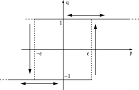
lineζ·Dω. Hence, we prefer to approximate thesignfunction in a different way. We maintain the discontinuity but we introduce a sort of delay in the switching. This is done by replacing the sign function by the delayed thermostathεdescribed in the Appendix. Let us denote by byϕan odd function onW taking only the values 1 and−1 and such thatϕ(ω) =sign(C2). We then consider the objective function
g4(ζ, η, µ, ω) =
k+ 1 2
° ° ° °
ζ+Dω
k
° ° ° °
2
+ 1
2kkµ−Dωk
2
+C1kDωk2+C2ηϕ(ω), (24)
where the new state variableη is subject to the evolution
η(t) =hε[z(t)·Dω, η0](t).
We have then introduced the new state variable η, which can only take the values 1 and −1 (the output of the thermostat) and whose evolution is subject to ”logic rules”, and not to ”differential rules”. That is we are considering a hybrid problem. Also note thatg4 is now continuous with respect to the state variables ζ
and η. However note that the discontinuity in the state is not definitely disappeared. It is now present in the evolution of the variables η which switches between two values. But such a switching is governed by the delayed thermostatic rule which allows us to say that switchings cannot accumulate in finite time (no Zeno phenomenon). Note that now we have two switching lines forη: the lineζ·Dω=εonly for switching up (from −1 to 1), and the lineζ·Dω=−εonly for switching down (from 1 to−1). Unfortunately, even if the objective functiong4 seems good for the maximization problem in ω with the saturated control, it is no more suitable
for the differential game problem. Indeed it may happen that, for particular values ofζ and η, the optimal choice of the minimization is to force the trajectory to cross one of the switching line, and to do that a different control from the linear saturated one may be necessary (recall that our final goal is to have the optimality of the saturated control, regardless of the behavior of the demand).
Fourth guess forg. The above outlined difficulty comes from the fact that the function ”distance ofζ from
±(Dω)/k”, where the sign±depends on which the maximizing ω is, is not continuous through the switching lines ζ·Dω = ±ε (note that it is instead continuous through the switching line ζ·Dω = 0, in the case of thesign function instead of the delayed relay). Hence we introduce a further term in the objective function which counts the number of switchings and, in some sense, makes that distance function continuous through the switching lines. The new objective function is (see Remark 3.1 for the meaning of the constant (2ε)/k)
g5(ζ, η, σ, µ, ω) =
k+ 1 2
° ° ° °
ζ+Dω
k
° ° ° °
2
+ 1
2kkµ−Dωk
2
+C1kDωk2
+C2ηϕ(ω)−sign(C2)
2ε kσ,
(25)
where the new state variableσ belongs to IN, and its discrete evolution is subject to a delayed switching rule given by (the term between parentheses can be expressed as the half of the total variation ofη in [0, t])
σ(t) =σ0+ (number of switchings of η in [0, t]).
3.
Formulation of the problems
In the following, byg(ζ, η, σ, µ, ω) we intend the functiong5as in (25), andT is the target set defined in (6).
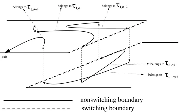
We define the following sets for the state variables (ζ, η, σ)∈ T × {−1,1} ×IN. For every fixedσ∈IN we define:
T1,σ =
n
(ζ,1, σ)¯¯
¯ζ∈ T, ζ·Dω≥ −ε o
,
T−1,σ =
n
(ζ,−1, σ)¯¯
¯ζ∈ T, ζ·Dω≤ε o
ζ
nonswitching boundary
switching boundary
belongs to
belongs to belongs to
belongs to
τ
τ
τ
τ
1,σ 1,σ+2
−1,σ+3 1,σ+4
[image:9.595.147.452.116.307.2]belongs to
τ
−1,σ+1 exitFigure 1. Switching evolution, starting fromζ, which exits from the nonswitching boundary after four switchings.
or, more generally, for every fixedη∈ {−1,1} andσ∈IN :
Tη,σ=
n
(ζ, η, σ)¯¯
¯ζ∈ T, η(ζ·Dω)≥ −ε o
.
For every initial state (ζ, η0, σ0)∈ Tη0,σ0, the controlled dynamical system is
z′(t) =u(t)−Dω(t), η(t) =hε[z(·)·Dω;η0](t),
σ(t) =σ0+ (number of switchings ofη in [0, t]),
z(0) =ζ.
(26)
We can say thatTη,σ is the set such that a trajecotry of (26), starting from (ζ, η, σ)∈ Tη,σ, does not incur in
any switching ofη(·) andσ(·) (i.e. switching of the thermostathε) until it remains inside Tη,σ (see Figure 1).
Note that, if we start from (ζ, η0, σ0)∈ Tη0,σ0, and if the evolution ofz(·) remains insideT for all the times,
then we certainly have
(z(t), η(t), σ(t))∈ [
n∈IN
T(−1)nη0,σ0+n.
Finally we consider the following exit-cost which acts when the trajectoryz(·) leaves the closed target T (note that the evolution ofz(·) is not subject to the evolution ofη andσ):
ψ(ζ, η, σ) =1 2
° ° ° °
ζ+sign(C2)ηDω
k
° ° ° °
2
+C1kDωk2+|C2| −sign(C2)2ε
kσ.
Remark 3.1. Note that, since the dynamicsµ−Dω is bounded, then, for passing from one switching line to the other, it is necessary to spend at least a timeτ >0 independently from the initial position on one of the two switching lines and from the controlsµandω. Moreover, in that case of the saturated controlµ(·) =−kz(·), for every initial state (ζ, η0, σ0) there exists a sequence of controlswδ(·) for the demand such that the corresponding
costs converge to ψ(ζ, η0, σ0), as δ → 0+. For instance, if C2 > 0, let us fix δ > 0 and start with w ≡η0ω
until t1+δ where t1 is the first switching instant for the trajectoryz(·) (it coincides with the reaching time
of the switching lineζ·Dω = −η0ε, which happens in a finite time). At the instant t1 the trajectory (η, σ)
direction, and the system goes on in this way for all the time. At every switching instant, the objective function
g¡
z(t), η(t), σ(t),−kz(t), η(t)ω¢
has a decrement of the quantity −(2ε)/k in its term containing the switching variableσwhich, via integration in the time up to +∞, is exactly compensated (modulo a quantity which goes to zero asδgoes to zero) by the increment in the quadratic part ¡
(2k+ 1)kz(t) +η(t)Dω/kk2¢
/2 (−(2ε)/k is equal to half of the difference between the square distances of a point on the switching line from the two points ±(Dω)/k). Hence, just a direct calculation proves the guess.
3.1.
Maximization problem.
When the control u ∈ U is fixed equal to the linear saturated control −kz(·), we have the maximization problem inw∈W given by the exit-time problem:
V(ζ, η, σ) = max
w∈W
Z t
0
e−sg(z(s), η(s), σ(s),−kz(s), w(s))ds
+e−tψ(z(t), η(t), σ(t)), t=tζ,w
wheretζ,w is the first exit time ofz(·) from the targetT, under the demand w. Since there exists a minimum time interval in order to pass from one switching line to the other (see remark 3.1), then, starting from any point (ζ, η, σ), with any controls, the cost is bounded (i.e. the integral converges, even if the trajectory z(·) never exits fromT). Indeed, what may be not bounded ingis the variableσwhich, if we have infinitely many switchings, goes to +∞. However, due to the uniform delay in time for every possible switching, and due to the presence of the discount exponential factore−t, the integral converges anyway.
Let us denote byintT and by∂T respectively the interior and the boundary ofT (as subset of IRn) For every (η, σ)∈ {−1,1} ×IN fixed we denote the interior ofTη,σ (”interior” with respect toζas subset of IR× {η} × {σ})
intTη,σ={(ζ, η, σ)
¯ ¯
¯(ζ, η, σ)∈ Tη,σ, ζ ∈intT, η(ζ·Dω)>−ε)},
For every (η, σ)∈ {−1,1} ×IN, the boundary ofTη,σ (”boundary” with respect toζas subset of IR× {η} × {σ})
is split in two parts (nonswitching boundary and switching boundary respectively, see the figure)
∂Tns
η,σ={(ζ, η, σ)
¯ ¯
¯(ζ, η, σ)∈ Tη,σ, ζ ∈∂T, η(ζ·Dω)>−ε},
∂Ts
η,σ={(ζ, η, σ)
¯ ¯
¯(ζ, η, σ)∈ Tη,σ, η(ζ·Dω) =−ε} Finally, we define
ˆ T = [
n∈IN
T1,n∪
[
n∈IN
T−1,n,
Since the delayed thermostat satisfies a suitable “semigroup property” (see Visintin [25]), the Dynamic Programming Principle holds: for every (ζ, η, σ)∈Tˆ, and for everyt >0 we have
V(ζ, η, σ) = sup
w∈W
à Z t
0
e−sg(z(s), η(s), σ(s),−kz(s), w(s))ds+e−tV(z(t), η(t), σ(t)) !
, (27)
wheret= min(t, tζ,w).
Proposition 3.2. The value functionV is continuous on Tˆ, i.e. separately on everyTη,σ.
Proof. Note that, forεsufficiently small, the points on the switching lines are totally controllable. Indeed,
for instance, the normal to the lineζ·Dω=εis of course given byDω, and, ifζis on that line, we have
(−kζ−Dω)·Dω <0<(−kζ+Dω)·Dω (28) where−kζ−Dω, and−kζ+Dωare the two possible dynamics. Moreover, for every initial point(ζ, η, σ)∈∂Tns
η,σ,
Tη,σthrough∂Tη,σns, and hence the exit-costψdoes not play a true role. The trajectory may exit fromTη,σ only
through the switching boundary∂Ts
η,σ. That is tζ,ω = +∞for allζ ∈ T and ω Hence, the only fact that may
cause discontinuity is the presence of the two switching linesζ·Dω=εandζ·Dω=−ε(which act as switching line only ifη(t) =−1 and η(t) = 1 respectively). However, the total (inward/outward) controllability on that lines and the fact that two possible subsequent switching time are delayed at least by an independent positive time makeV continuous anyway, as can be proved by standard techniques. ¤
For every (η, σ)∈ {−1,1} ×IN, we consider the following Hamiltonian in IRn×IRn
Hη,σ(ζ, p) = min
ω∈W{−(−kζ−Dω)·p−g(ζ, η, σ,−kζ, ω)}
For every (η, σ)∈ {−1,1}×IN, we consider the following Hamilton-Jacobi-Bellman problem inTη,σwith (partial)
boundary condition, which, for a generic solution (ζ, η, σ)7→ v(ζ, η, σ)), (which of course depends only on ζ, sinceη andσare fixed inTη,σ) is written as
½
v(ζ, η, σ) +Hη,σ(ζ,∇ζv(ζ, η, σ)) = 0 inintTη,σ, v(ζ, η, σ) =ψ(ζ, η, σ) on∂Tns
η,σ
(29)
where∇ζ means the gradient with respect toζonly. Note that the boundary condition is ”partial” since it is
imposed only on the nonswitching boundary∂Tns
η,σ. We call (29)HJBη,σ.
Proposition 3.3. Standing all the hypotheses already assumed, the value function V of our maximization
problem is the unique continuous function onTˆ satisfying both
V(ζ, η, σ)−V(ζ, η, σ+ 1) =−sign(C2)
2ε
k, (30)
V(ζ, η, σ)≥max{ψ(ζ, η, σ), V(ζ,−η, σ+ 1)} ∀ (ζ, η, σ)∈∂Ts
η,σ∩∂Tη,σns, (31) and finally which solves the following problem
∀(η, σ)∈ {−1,1} ×IN,V solves the following in the viscosity sense:
½
V solvesHJBη,σ (29),
V(ζ, η, σ) =V(ζ,−η, σ+ 1) on∂Ts η,σ.
(32)
Remark 3.4. We refer to Proposition 6.1, regardingTη,σ as Ω,∂Tη,σs as (∂Ω)1, and∂Tη,σns as (∂Ω)ˆ1. By virtue
of (28), which in our case also implies that the analogous of (48) holds, for every (η, σ) fixed and for every continuous functionhdefined on∂Ts
η,σ, satisfying
h(ζ, η, σ)≥ψ(ζ, η, σ) on∂Ts
η,σ∩∂Tη,σns
there exists a unique continuous functionv defined onTη,σ which solves the problem
½
v solves HJBη,σ (29),
v(ζ, η, σ) =h(ζ, η, σ) on∂Ts η,σ,
and it coincides with the value function of the maximization problem inTη,σ with exit cost given byψon∂Tη,σns
(which does not play any role by (47)) and byhon∂Ts
η,σ. However, this fact does not immediately implies the
uniqueness for the Hamilton-Jacobi problem as in the proposition above, since there the boundary conditions (i.e. the exit-costs) are mutually exchanged on the switching boundaries, i.e. they are part of the solution. However, such a uniqueness result for every (η, σ) fixed will be of course used in the proof.
Proof of Proposition 3.3. By Proposition 3.2, the value functionV of our maximization problem is continuous
on ˆT. Moreover it also satisfies (30). Indeed, all the initial states (ζ, η, σ+n), with n∈IN, are exactly in the same situation with respect to the future evolution and to the costg, except for the value −sign(C2)(2ε)/k.
It solves (31) because, by definition ofψ, by the argumentation of Remark 3.1, and by the controllability (46) we have that for all (ζ, η, σ)∈∂Ts
V(ζ, η, σ)≥V(ζ,−η, σ+ 1)
V(ζ,−η, σ+ 1)≥ψ(ζ,−η, σ+ 1) =ψ(ζ, η, σ). (33)
It also solves (32). Indeed, for every (ζ, η, σ)∈ Tη,σand for every controlw∈W let us denote bytw≤+∞the
corresponding exit-time fromTη,σ, (recall that the exit time ofz(·) fromT is always equal to +∞,tζ, w= +∞).
Let us fix (ζ, η, σ)∈ Tη,σ, and suppose that, for everyε >0 there exists a control wε which is ε-optimal and
such thattwε is finite (if not, the case is easier). Then, forδ >0 sufficiently small, we have (using the definition ofV, the inequality (33) and the Dynamic Programming Principle (27), also recall that, by definition of the switching rule for the delayed thermostat, at the switching instanttw the switching is not yet happened)
Z twε+δ
0
e−sg(z(s), η(s), σ(s),−kz(s), wε(s))ds
+e−twε
V(z(twε+δ),−η, σ+ 1) +ε ≥V(ζ, η, σ)
≥ sup
w∈W
à Z tw
0
e−sg(z(s), η, σ,−kz(s), w(s))ds+e−twV(z(tw), η, σ) !
≥ sup
w∈W
à Z tw
0
e−sg(z(s), η, σ,−kz(s), w(s))ds+e−tw
V(z(tw),−η, σ+ 1)
!
.
Taking the limitδ→0+, using the continuity ofV and the arbitrariness ofε >0 we get, for every (ζ, η, σ)∈ T
η,σ
V(ζ, η, σ) = sup
w∈W
à Z tw
0
e−sg(z(s), η, σ,−kz(s), w(s))ds+e−twV(z(tw),−η, σ+ 1)
!
.
This means that on everyTη,σ, V is the value function of the maximization problem with exit cost fromTη,σ
given byψon∂Tns
η,σ(which, however, does not play any role) and byV(·,−η, σ+1) on∂Tη,σs . Hence, by Remark
3.4,V satisfies the Hamilton-Jacobi problem (32).
Now let us prove the uniqueness. Let us consider two continuous functionsf, h defined on ˆT which satisfy the same inequalities (30), (31) saitsfied byV, and the Hamilton-Jacobi problem (32). We are going to prove thatf =h. For every (η, σ) fixed, f and hare, onTη,σ (see Remark 3.4), the value function of two exit-time
maximization problems which differs from each other only for the exit-costs on the switching boundary∂Ts η,σ.
Those two exit-costs are given respectively by f(ζ,−η, σ+ 1) and h(ζ,−η, σ+ 1). The same argumentation shows that, onT−η,σ+1 f and hare the value functions of two exit-time maximization problems which differ
from each other only for the exit costs on the switching boundary∂Ts
−η,σ+1. Now, recalling that we need to
spend at least an independent time τ > 0 in order to pass from one switching boundary to the other, and recalling (30) we get, for every fixed (η, σ)
sup
(ζ,η,σ)∈Tη,σ
|f(ζ, η, σ)−h(ζ, η, σ)|
≤ sup
(ζ,η,σ)∈∂Ts η,σ
|f(ζ,−η, σ+ 1)−h(ζ,−η, σ+ 1)|
≤e−τ sup
(ζ,−η,σ+1)∈∂Ts −η,σ+1
|f(ζ, η, σ+ 2)−h(ζ, η, σ+ 2)|
≤e−τ sup
(ζ,η,σ+2)∈Tη,σ+2
|f(ζ, η, σ+ 2)−h(ζ, η, σ+ 2)|
=e−τ sup
(ζ,η,σ)∈Tη,σ
|f(ζ, η, σ)−h(ζ, η, σ)|
3.2.
The MinMax problem.
Here the problem is given by the (lower) value function
˜
V(ζ, η, σ) = inf
γ∈Γwsup∈W
Z ˜t
0
e−sg(z(s), η(s), σ(s), γ[w](s), w(s))ds
+e−˜tψ(z(˜t), η(˜t), σ(˜t)), ˜t=tζ,γ,w
where Γ is the set of non-anticipative strategies for the first player (the minimizing one), andtζ,γ,w ≤+∞is the first exit time ofz(·) from the closed of the targetT under the demandwand the strategyγ.
Also in this case, the Dynamic Programming Principle holds: for every (ζ, η, σ)∈Tˆ, and for everyt >0 we have
˜
V(ζ, η, σ) = inf
γ∈Γwsup∈W
à Z t
0
e−sg(z(s), η(s), σ(s), γ[w](s), w(s))ds+e−tV˜(z(t), η(t), σ(t))
!
, (34)
wheret= min(t, tζ,γ,w).
Proposition 3.5. The value functionV˜ is continuous in Tˆ.
Proof. Note that, by (5), the dynamical system ˙z=u−Dwis completely controllable inzby the first player,
whichever is the controlω used by the second player. That is, for every (ζ, η, σ)∈∂Tns
η,σ∪∂Tη,σs , there exists
two controlsµ1, µ2 ∈ U such that for everyω ∈W the fieldµ1−Dω, when applied in ζ, is strictly inward in
intTη,σ (i.e. (ζ+ν(µ1−Dω), η, σ)∈intTη,σ forν >0 sufficiently small), and the fieldµ2−Dω, when applied
inζ, is strictly outward fromTη,σ (i.e. (ζ+ν(µ2−Dω), η, σ)6∈ Tη,σ forν >0).
Such a total controllability on the boundary and on the switching lines, together with the delay property of the switching instants, make the value function ˜V continuous, as can be proved by techniques similar to those of the proof of Proposition 6.2. ¤
For every (η, σ), we have the Hamiltonian, defined in IRn×IRn,
˜
Hη,σ(ζ, p) = min
ω∈Wmaxµ∈U{−(µ−Dω)·p−g(ζ, η, σ, µ, ω)}.
For every (η, σ) ∈ {−1,1} ×IN, we consider the Hamilton-Jacobi-Isaacs problem in Tη σ with (partial)
boundary condition which, for a generic solution (ζ, η, σ) 7→ v(ζ, η, σ)), (which of course depends only on ζ, sinceη andσare fixed inTη,σ) is written as
½
v(ζ, η, σ) + ˜Hη,σ(ζ,∇ζv(ζ, η, σ)) = 0 in Tη,σ, v(ζ, η, σ) =ψ(ζ, η, σ) on∂Tns
η,σ,
(35)
where∇ζ means the gradient with respect toζonly. Note that the boundary condition is ”partial” since it is
imposed only on the nonswitching boundary ofTη,σ. We call (35) HJIη,σ˜ .
Proposition 3.6. Standing all the hypotheses already assumed, the value functionV˜ of our minmax problem
is the unique continuous function onTˆ which satisfies (30) and the following inequality
˜
V(ζ, η, σ)≤min{ψ(ζ, η, σ),V˜(ζ,−η, σ+ 1)} ∀ (ζ, η, σ)∈∂Ts
η,σ∩∂Tη,σns, (36) and finally which solves the following problem
∀(η, σ)∈ {−1,1} ×IN,
˜
V solves the following in the viscosity sense:
½ ˜
V solves HJIη,σ˜ (35),
˜
V(ζ, η, σ) = ˜V(ζ,−η, σ+ 1) on∂Ts η,σ.
Remark 3.7. First, let us note that, for every (η, σ) fixed, the boundary condition inHJIη,σ˜ (35) is now playing a true role (despite to what happens for the maximization problem) since, on the nonswitching boundary∂Tns
η,σ,
there are strategies for the first player that make the trajectory exit (by virtue of (5)). Moreover, (5) also implies that the point on∂Ts
η,σ∩∂Tη,σns are totally controllable by the first player, and also that there exist strategies
for the first player such the analogous of (55) holds. Hence, by Proposition 6.2, for every (η, σ) fixed, and for continuous functionhdefined on the switching boundary∂Ts
η,σ, such that
h(ζ, η, σ)≤ψ(ζ, η, σ) on∂Ts
η,σ∩∂Tη,σns
there exists a unique continuous function ˜v defined onTη,σ such that
˜
v(ζ, η, σ)≤min{ψ(ζ, η, σ), h(ζ, η, σ)} on∂Ts
η,σ∩∂Tη,σns
and such that solves the problem
½ ˜
v solvesHJIη,σ (35),
˜
v(ζ, η, σ) =h(ζ, η, σ) on∂Ts η,σ,
Such a unique function ˜v coincides with the value function of the minmax problem inTη,σ with exit cost given
byψ on∂Tns
η,σ and byhon∂Tη,σs . Final considerations as in Remark 3.4 then follow.
Proof of Proposition 3.6. Let us note that, by the controllability on the boundary, and by the definition ofψ,
also in this case ˜V satisfies (36). Moreover, also in this case ˜V satisfies (30). The fact that ˜V satisfies (37), and that it is the unique solution comes, via Remark 3.7, by the same argumentation as in the proof of Proposition 3.3. In particular, using the Dynamic Programming Principle (34), suitably arguing as for the maximization problem, we have, for every (ζ, η, σ)∈∂Ts
η,σ∩∂Tη,σns (here tγ,w is the first switching instant of the trajectory)
sup
w∈W
Ã
Z tγε ,w+δ
0
e−sg(z(s), η(s), σ(s), γε[w](s), w(s))ds
+e−tγε ,w+δ˜
V(z(tγε,w+δ),−η, σ+ 1)
´
−ε
≤V˜(ζ, η, σ)
≤inf
γ∈Γwsup∈W
à Z tγ ,w
0
e−sg(z(s), η(s), σ(s), γ[w](s), w(s))ds+e−tγ ,w ˜
V(z(tγ,w), η, σ)
!
≤inf
γ∈Γwsup∈W
à Z tγ ,w
0
e−sg(z(s), η(s), σ(s), γ[w](s), w(s))ds+e−tγ ,w ˜
V(z(tγ,w),−η, σ+ 1)
!
¤
4.
Robustness
In this section, we proof the robustness of the linear saturated control in the sense of Definition 0.1. This is done exhibiting a continuous function on ˆT which solves both problems (32) and (37).
Proposition 4.1. For suitable choices of the constantC1 andC2, the function
φ(ζ, η, σ) =1 2
° ° ° °
ζ+sign(C2)η
Dω k
° ° ° °
2
+C1kDωk2+|C2| −sign(C2)
2ε kσ, solves both problems (32) and (37).
Proof. It is evident thatφis continuous and that it satisfies (30), (31) and (36). Moreover, also the boundary
condition are satisfied (even in the classical sense: point by point). Now, let us note that, for every (η, σ) fixed,
φis of class C1 (with respect toζ) inintT
∇ζφ(ζ, η, σ) =ζ+sign(C2)ηDω
k .
Hence, we have to findC1>0 andC2∈IR such that, for every (η, σ), the following holds in the classical sense:
φ(ζ, η, σ) +Hη,σ(ζ,∇ζφ(ζ, η, σ)) = 0, in intTη,σ, φ(ζ, η, σ) + ˜Hη,σ(ζ,∇ζφ(ζ, η, σ)) = 0. in intTη,σ.
By (21), by the compactness ofT,U andW, the values ofC1>0 and of|C2|are easily constructed (recall also
the definition ofϕwhich appears in the objective functiong=g5 (25)) For instance, we can take, without any
pretension of sharpness
|C2| ≥2 max
ζ∈T,µ∈U,ω∈W,η∈{−1,1}|f(ζ, η, µ, ω)|,
C1≥ max
ζ∈T,µ∈U,ω∈vertW,ω6=±ω,η∈{−1,1}
f(ζ, η, µ,±ω)−f(ζ, µ, ω) kDωk2− kDωk2 ,
wherevertW is the set of the vertices ofW and
f(ζ, η, ω, ω) =−(µ−Dω)·(ζ+ηDω k )−
k+ 1 2
° ° ° °ζ+
Dω k
° ° ° °
2
− 1
2kkµ−Dωk
2,
¤
Proposition 4.2. If C1 and C2 are the ones outlined in Proposition 4.1, then the linear saturated control is robustly optimal in the sense of Definition 0.1.
Proof. Given Proposition 4.1 and the uniqueness results of the previous section, the conclusion immediately
follows, since we haveV = ˜V =φ. ¤
Remark 4.3. Whenεgoes to zero, the thermostathεtends to thesignfunction. Moreover, the value function
V and ˜V (which are equal by the way), on everyTη,σ, uniformly converge to the function
V0(ζ, η) = 1
2 ° ° ° °
ζ+sign(C2)ηDω
k
° ° ° °
2
+C1kDωk2+|C2|,
which does not depend onσ anymore, and with η =sign(ζ·Dω). One may ask whether V0 is the value for
both the maximization problem and the minmax problem with the thermostat replaced by thesign function (something as in the ”Second guess” paragraph). Unfortunately this is not true. A probably correct guess is that the almost optimal trajectories for the problems with the thermostathε(which, for the case C2>0, are
2
3
4
5 1
8
1
2 5
6
4
7
[image:16.595.229.369.135.242.2]9 3
Figure 2. Example of a system with 5 nodes and 9 arcs.
0 100 200 300 400 500 600 700 −2
[image:16.595.211.380.307.444.2]0 2 4 6 8 10
Figure 3. State trajectory for the system of Fig. 2. Chattering around the hyperplaneH is due to the discontinuous behavior ofω that jumps between ¯ω and−ω¯.
5.
Numerical simulations
5.1.
First guess for
g
We considerg2 as in (22) and the system with 5 nodes and 9 arcs displayed in Fig. 2. We take matrixD as
follows
D=
0 1 0 0 0
0 0 0.5 0 0 −0.1 0 0.5 0 0 −0.2 0 0 0 0
0 0 0 0 0
0 0 0.5 0 0 0.1 0 0 1 0 0.6 1 1 0 0 0.4 0 0 1 1
, (38)
and ¯ω= [0 1 1 1 1]′.
Figure 3 displays the time plot of the state trajectory. We have 9 state variables (as many as the arcs of the network). Chattering around the hyperplaneHis due to the discontinuous behavior ofω that jumps between ¯
[image:16.595.223.374.561.670.2]−10 −8 −6 −4 −2 0 2 4 6 8 10 −10 −8 −6 −4 −2 0 2 4 6 8 10
Figure 4. State trajectory in the phase plane from different initial states (circles) forg3as in (23) andC2<0. In evidence the two equilibria±Dkω¯ =±[10 10]′ (star).
−10 −5 0 5 10
−10 −5 0 5 10
z1(t)
z2
(t)
−10 −5 0 5 10
−10 −5 0 5 10
z1(t)
z2
(t)
−10 −5 0 5 10
−10 −5 0 5 10
z1(t)
z2
(t)
−10 −5 0 5 10
−10 −5 0 5 10
z1(t)
z2
(t)
Figure 5. State trajectory in the phase plane from different initial states (circles). In evidence the two equilibria ±Dω¯
k =±[10 10]
′ (star). (Top left) g
3 as in (23) andC2>0; (top right) g4 as in (24) andǫ= 0.2; (bottom left)g4 as in (24) andǫ= 0.5; (bottom right)g4as in (24) and
ǫ= 1.
5.2.
Second and third guesses for
g
We considerg3 as in (23) and again the system with 1 node and 2 arcs displayed in Figure 1. The incidence
matrix isB= [1 1] and we take matrixD= [1/2 1/2]′.
In Fig. 4 and 5 (top left), we plot the state trajectory in the phase plane for the two casesC2>0 andC2<0
and from different initial states (circles) as
z(0) = · 5 5 ¸ , · 5 −5 ¸ , · −5 −5 ¸ , · −5 −5 ¸ , · 7.5 2.5
¸
,
· 2.5 −5
¸
,
·
−2.5 −5
¸
,
·
−5 2.5
¸
,
· 2.5 7.5
¸
. (39)
In evidence the two equilibria±Dω¯
k =±[10 10]
′ (star).
WhenC2<0 (see Fig. 4) we haveω=−ω¯ and the trajectories remain in the same half-space reaching the
[image:17.595.187.410.309.492.2]0 200 400 600 800 −4
−2 0 2 4 6 8 10
t
z(t)
0 200 400 600 800
−4 −2 0 2 4 6 8 10
t
z(t)
0 200 400 600 800
−4 −2 0 2 4 6 8 10
t
z(t)
0 200 400 600 800
−4 −2 0 2 4 6 8 10
t
[image:18.595.186.409.122.303.2]z(t)
Figure 6. State trajectory for the system of Fig. 2 for different values ofǫ: (top left)ǫ = 0 and g3 as in (23), (top right)ǫ= 0.8; (bottom left) ǫ= 2; (bottom right)ǫ = 5. Chattering around the hyperplane Hincreases withǫ.
Differently, whenC2>0 (see Fig. 5 (top left)) we haveω= ¯ωand the trajectories try to leave one half-space
to reach the equilibrium of the other half-space. The trajectory do not reach the equilibrium because of the switching behavior ofω across the hyperplaneζ·Dω¯ = 0.
Figure 5 also displays the state trajectories when g4 is as in (24) and demand performs according to the
delayed thermostat behavior. We considered different values of ǫ: (top right)ǫ = 0.2; (bottom left) ǫ = 0.5; (bottom right)ǫ= 1.
Finally, we carried out simulations for the system with 5 nodes and 9 arcs displayed in Fig. 2 wheng4 is as
in (24) and demand performs according to the delayed thermostat behavior. Again, we have 9 state variables (as many as the arcs of the network). Fig. 6 displays the time plot of the state trajectory for different values of
ǫ: (top left)ǫ= 0 andg3 as in (23), (top right)ǫ= 0.8; (bottom left)ǫ= 2; (bottom right)ǫ= 5. Chattering
around the hyperplaneHis due to the discontinuous behavior ofω that jumps between ¯ω and−ω¯. Amplitude of chattering increases withǫ.
6.
Appendix
6.1.
Some facts on Hamilton-Jacobi, viscosity solutions and control problems
For the general theory and results concerning viscosity solutions for Hamilton-Jacobi equations see Bardi-Capuzzo Dolcetta [4]. Here, we state and prove some relatively new results exposed in a manner which is suitable for our purposes.
6.1.1. Viscosity solutions with boundary conditions in the viscosity sense
Let us give
Ω⊂IRn open, bounded, satisfying a uniform cone property (see [4] eq: IV (5.21)),
F : IRn×IRn→IR a continuous function, ξ:∂Ω→IR a function. (40)
We say that a continuous functionv : Ω →IR is a viscosity solution of the boundary value problem, with
½
v(x) +F(x,∇v(x)) = 0 in Ω,
v=ξ on∂Ω,
ifv is a viscosity solution of the Hamilton-Jacobi equation in Ω (i.e. the first line) and, for everyx∈∂Ω and for every continuously differentiable functionϕ: Ω→IR we have
v−ϕhas a local maximum inxwith respect to Ω =⇒ min³v(x)−ξ∗(x), v(x) +F(x,∇ϕ(x)) ´
≤0;
v−ϕhas a local minimum inxwith respect to Ω =⇒ max³v(x)−ξ∗(x), v(x) +F(x,∇ϕ(x))´≥0,
whereξ∗ andξ∗ are respectively the lower semicontinuous envelope and the upper semicontinuous envelope:
ξ∗(x) = lim inf
y→x,y∈∂Ωξ(y), ξ
∗(x) = lim sup
y→x,y∈∂Ω
ξ(y), ∀x∈∂Ω.
6.1.2. Optimal control problems with exit-time
Here, to not introduce much more notation,W andW are the same as in (4), (7). Moreover Ω andξare as in (40), but we further assume that there existm C2-functionsθi,i= 1, . . . , m, such that
Ω =nx∈IRn¯¯
¯θi(x)>0 ∀i= 1, . . . , m o
. (41)
Moreover, we use the following notation
(∂Ω)1=nx∈IRn¯¯
¯θ1(x) = 0 o
⊆∂Ω, (∂Ω)ˆ1=
n
x∈IRn¯¯
¯θi(x) = 0i= 2, . . . , m o
⊆∂Ω, (42)
and suppose that ξ : ∂Ω → IR is continuous on (∂Ω)1 and on (∂Ω)ˆ1 separately and it is globally upper
semicontinuous on∂Ω, i.e. for allx∈(∂Ω)ˆ1∩(∂Ω)1
lim
y→x,y∈(∂Ω)ˆ1
ξ(y) =ξ∗(x)≤ξ∗(x) = lim
y→x,y∈(∂Ω)1
ξ(y). (43)
Finally
f : IRn× W →IRn, ℓ: IRn× W →IR,
are two bounded Lipschitz continuous functions. We now consider the controlled dynamical system in IRn
½
y′(t) =f(y(t), w(t)) t >0,
y(0) =x∈Ω, (44)
and the payoff (here and in the sequel, by continuity,ξ∗(x) =ξ∗(x) =ξ(x) ifx6∈(∂Ω)1∩(∂Ω)ˆ1)
J(x, w) = Z tx,w
0
e−tℓ(y(t), w(t))dt+e−tx,wξ∗(y(tx,w)),
wherey(·) is the unique trajectory of (44) withw∈W, andtx,w is the first exit time of the trajectory from Ω:
tx,w= infnt≥0¯¯
¯y(t)6∈Ω o
, (45)
with the convention inf∅= +∞(ande−∞ξ= 0).
Proposition 6.1. Standing all the above hypotheses, if on(∂Ω)1 the dynamics is totally controllable i.e.:
∀x∈(∂Ω)1, ∃ω1, ω2∈ W such that
f(x, ω1)is strictly entering inΩatx,
f(x, ω2)is strictly entering in the complementary ofΩatx,
on(∂Ω)ˆ1 we have only strictly inward admissible fields, i.e.:
f(x, ω)is strictly entering inΩatx∀x∈(∂Ω)ˆ1, ∀ω∈ W, (47)
and moreover if for everyx∈(∂Ω)ˆ1there exists a controlw∈W such that the corresponding trajectory starting
fromxreaches(∂Ω)1 in a lap of timet satisfying
t≤Cdist(x,(∂Ω)1), (48)
withC >0 independent onx, then the value function of the maximization problem
v(x) = sup
w∈W
J(x, w)
is continuous in Ω, and it is the unique viscosity solution of the Hamilton-Jacobi-Bellman boundary value
problem (with boundary condition in the viscosity sense)
(
v(x) + min
ω∈W{−f(x, ω)· ∇v(x)−ℓ(x, ω)}= 0 inΩ
v=ξ∗ on∂Ω, (49)
satisfying the condition
v(x)≥ξ∗(x) ∀x∈(∂Ω)1∩(∂Ω)ˆ1 (50)
Proof. The proof suitably adapts standard techniques to our situation. We do not report it. However, we
are going to report a sketched proof for the analogous case of differential games. ¤
6.1.3. Differential games with exit-time
Here, again,W, W are as in (4), (7). MoreoverU andU are as in (3), (7), Γ is as in (8), Ω andξare as in (40), satisfying also (41), (42), and moreoverξ:∂Ω→IR is continuous on (∂Ω)1 and on (∂Ω)ˆ1 separately and
it is globally lower semicontinuous on∂Ω, i.e. for allx∈(∂Ω)ˆ1∩(∂Ω)1
lim
y→x,y∈(∂Ω)1ξ(y) =ξ∗(x)≤ξ
∗(x) = lim
y→x,y∈(∂Ω)ˆ1
ξ(y). (51)
Note the difference between (51) and (43): the role of (∂Ω)1 and (∂Ω)ˆ1 are mutually exchanged. Finally
˜
f : IRn× U × W →IRn, ℓ˜: IRn× U × W →IR,
are two Lipschitz continuous functions. We now consider the controlled dynamical system in IRn
½
y′(t) = ˜f(y(t), γ[w](t), w(t)) t >0,
y(0) =x∈Ω, (52)
and the payoff
˜
J∗(x, γ, w) = Z tx,γ ,w
0
e−tℓ˜(y(t), γ[w](t), w(t))dt+e−tx,γ ,wξ
∗(y(tx,γ,w)), (53)
wherey(·) is the unique trajectory of (52) withγ∈Γ w∈W, and tx,γ,w is the first exit time of the trajectory from Ω (similarly defined as in (45)).
Proposition 6.2. Standing the above hypotheses, if the dynamics is totally controllable by the first player (the minimizing one) on the points of the boundary i.e.
∀x∈∂Ω, ∃µ1, µ2∈ U such that,∀ω∈ W,
˜
f(x, µ1, ω)is strictly entering inΩatx,
˜
f(x, µ2, ω)is strictly entering in the complementary ofΩatx,
moreover if for every x∈ (∂Ω)ˆ1 there exists a strategy γ ∈Γ such that, for every w∈ W, the corresponding
trajectory starting fromxreaches(∂Ω)1 in a lap of timet satisfying
t≤Cdist(x,(∂Ω)1), (55)
withC >0 independent onw∈W, then the (lower) value function of the minmax problem
˜
v(x) = inf
γ∈Γwsup∈W
˜
J∗(x, γ, w)
is continuous inΩ, and it is the unique continuous viscosity solution of the Hamilton-Jacobi-Isaacs boundary
value problem (with boundary condition in the viscosity sense)
( ˜
v(x) + min
ω∈Wmaxµ∈U n
−f˜(x, µ, ω)· ∇˜v(x)−ℓ˜(x, , µ, ω)o= 0 in Ω
˜
v=ξ∗ on ∂Ω,
(56)
satisfying the condition
˜
v(x)≤ξ∗(x) ∀x∈(∂Ω)1∩(∂Ω)ˆ1 (57)
Proof. v˜is continuous. The continuity of ˜vcomes from (54), (55), from the fact thatξis separately continuous
on (∂Ω)1 and (∂Ω)ˆ1, and also from the fact thatξ∗ is continuous on (∂Ω)1∩(∂Ω)ˆ1 (see (51)). In particular
note that (55) guarantees the (controlled in time) reachability of (∂Ω)1, where the values of the exit costξare (probably) lower than the values on (∂Ω)ˆ1, at least for points near to (∂Ω)1∩(∂Ω)ˆ1. Indeed, adapting a result
due to Soner [24] (see also Bagagiolo-Bardi [2] for a generalization to a polytopic case as (41)), there exist a timeτ >0 and a constantα >0 (both depending only on Ω and on ˜f via (54)) such that, for everyx∈Ω and for everyu∈U, there exists a controlu∈U such that
yx(t;u, w)∈Ω, ∀0≤t≤τ, ∀w∈W,
|Jτ(x, u, w)−Jτ(x, u, w)| ≤α sup
0≤t≤τ
dist³yx(t;u, w),Ω´, ∀w∈W, (58)
where yx(·;u, w) and yx(·;u, w) are respectively the trajectories of (52) with u and u as first control (i.e.
γ[w] ≡ u, γ[w] ≡u, respectively), and, in general, fort ≥0, Jt is the corresponding cost given only by the integral part of (53) up to the timet, independently whether the trajectory stays inside Ω or not. From (58), and standard estimates on the trajectories, we get the following
∀T >0, ∃CT >0 such that∀x, y,∈Ω, ∀(u, w)∈U×W
withyy(t;u, w)∈Ω∀0≤t≤T, ∃u∈U such that kyx(t;u, w)−yx(t;u, w)k ≤CTkx−yk ∀t∈[0, T],
kyx(t;u, w)−yy(t;u, w)k ≤CTkx−yk ∀t∈[0, T],
¯ ¯
¯JT(x, u, w)−JT(y, u, w) ¯ ¯
¯≤CTkx−yk.
(59)
Now, from (59), from the reachability condition (55), and again from the controllability condition (54), and from standard inequalities on the trajectories, we then get the following
∀δ >0 ∃Cδ>0 such that∀x, y∈Ω, ∀γ∈Γ, ∃γ∈Γ such that∀ w∈W
¯ ¯
¯J∗(x, γ, w)−J∗(y, γ, w) ¯ ¯
¯≤Cδkx−yk+δ.
(60)
To obtain (60), observe that all the estimates in (59) are independent onw∈W, and takeT >0 such that the possible remaining part of the cost J∗ in the time interval (T,+∞) is certainly less than δ/2 for every initial pointxand couple of controls (u, w). Then construct the strategyγ definingγ[w] by observing the trajectory
1
−1
p q
[image:22.595.228.367.123.213.2]ε −ε
Figure 7. Delayed thermostat with thresholds±ε.
easily get the continuity of ˜v. It is sufficient to argue by absurd and suppose that there exist a pointx∈Ω, a sequence{yn}n⊂Ω converging tox, andε >0 such that|˜v(x)−˜v(yn)| ≥εfor alln∈IN.
˜
v solves (56), (57). This fact is checked by standard techniques. In particular, observe that by the
control-lability hypothesis (54), ˜vcertainly satisfies (57). ˜
v is the unique solution of (56). We argue as in Bardi-Capuzzo Dolcetta [4] (Chapter V, Theorem 4.17).
The only difference here is that the boundary datum is discontinuous. However, the only possible discontinuous points are in (∂Ω)1∩(∂Ω)ˆ1. But there, condition (57) guarantees the applicability of the argument. ¤.
Remark 6.3. Differential games with exit time and/or state-constraints present, in general, the problem of devolving the responsability of exit and/or respecting the state-constraints to both players (see Evans-Ishii [17], Koike [19], Bardi-Koike-Soravia [5], Cardialaguet-Quincampoix-SaintPierre [11]). In the present case, the controllability condition (54) and the fact that we are only concerned with the lower value (first minimizing, then maximizing), make all the responsability and the faculty of exit and/or respecting the state-constraint be up to the first player only (the minimzing one). Uniqueness results for first order Hamilton-Jacobi equations with discontinuous boundary datum and/or discontinuous Hamiltonians are in general hard to get, see for instance Soravia [23] and Garavello-Soravia [18]. In the present paper, conditions (50), (57), and the approximation of the discontinuity by the delayed relay are of course useful. However, our goal is not to give a general result of uniqueness, but instead to have suitable uniqueness results in order to recognize given functions as the values of the optimal control and of the differential game. This is what we just do in Section 4.
6.2.
On the delayed thermostat
For more details on this subject we refer to Visintin [25]. Let us consider a continuous inputp: [0,+∞[→IR, a discontinuous outputq: [0,+∞[→ {−1,1}, and two different thresholds for the values ofp, let us say−εand
ε, withε >0, for whichqrespectively switches “down” from +1 to−1, and “up” from−1 to +1. We define
O:= (]− ∞,+ε]× {−1})∪([−ε,+∞[×{1})⊂IR2=:O−1∪ O1,
and we can think to the delayed switching as the evolution of the couple (p(·), q(·)) on the setOwith a suitable switching rule for switching from one branch to the other. More in details, we say thatqis the output of the delayed switching rule (or “delayed thermostat”, or “delayed relay”) with thresholds−ε, ε, inputu, and initial stateq0∈ {−1,1}, and we writeq(t) =hε[p, q0](t)∀t≥0, if (hereδis any positive number)
i) (p(t), q(t))∈ O ∀t≥0, q(0) =q0, (p(0), q0)∈ O
ii)q(t) = 1, p(·)≥ −εin [t, t+δ] =⇒q(·) is constant in [t, t+δ], iii)q(t) =−1, p(·)≤εin [t, t+δ] =⇒q(·) is constant in [t, t+δ].
instance, (p(t), q(t)) = (p(t),1) then certainlyp(t)≥ −εand a possible subsequent switching timeτ ∈[t,+∞[ is exactly the first exit time of the trajectoryp(·) from the closed set [−ε,+∞[, which is similarly defined as in (45). In particular, for the same example, the fact thatp(t) =−ε for some t ≥t, does not in implies any swithcing if the threshold is not crossed (i.e. ifp 6< −ε immediately after t). After any switching instant t,
q cannot immediately switch back, because phas to reach the other threshold. This implies the existence of exactly one output, even for fast oscillating inputs, i.e. no Zeno phenomenon.
References
[1] F. Bagagiolo, Minimum time for a hybrid system with thermostatic switchings, inHybrid Systems: Computation and Control, A. Bemporad, A. Bicchi, and G. Buttazzo (Eds.), Lecture Notes in Computer Sciences 4416, Springer-Verlag, Berlin (2007) 32-45.
[2] F. Bagagiolo, M. Bardi, Singular perturbation of a finite horizon problem with state-space constraints.SIAM J. Control Optim.
36(1998) 2040-2060.
[3] F. Bagagiolo, D. Bauso, Robust optimality of linear saturated control in uncertain linear network flows,Decision and Control, 2008. CDC 2008. 47th IEEE Conference on 9-11 Dec. 2008 Page(s):3676 - 3681.
[4] M. Bardi, I. Capuzzo Dolcetta,Optimal Control and Viscosity Solutions of Hamilton-Jacobi-Bellman Equations. Birkh¨auser, Boston (1997).
[5] M. Bardi, S. Koike, P. Soravia, Pursuit-evasion games with state constraints: dynamic programming and discrete-time approx-imation.Discrete Contin. Dyn. Syst.6(2000) 361-380.
[6] D. Bauso, F. Blanchini, R. Pesenti, Robust control policies for multi-inventory systems with average flow constraints.Automatica
42(8) (2006) 1255-1266.
[7] A. Bemporad, M. Morari, V. Dua, and E. N. Pistikopoulos, The explicit linear quadratic regulator for constrained systems. Automatica 38(1) (2002) 320.
[8] A. Ben Tal, A. Nemirovsky, Robust solutions of uncertain linear programs.Operations Research25(1) (1998) 1-13.
[9] D. P. Bertsekas, I. Rhodes, Recursive state estimation for a set-membership description of uncertainty.IEEE Trans. on Auto-matic Control16(2) (1971) 117-128.
[10] D. Bertsimas, A. Thiele, A Robust Optimization Approach to Inventory Theory.Operations Research54(1) (2006) 150-168. [11] P. Cardialaguet, M. Quincampoix, P. Saint-Pierre, Pursuit differential games with state constraints.SIAM J. Control Optim.
39(2001) 1615-1632.
[12] J. Casti, On the general inverse problem of optimal control theory.J. Optim. Theory Appl.32(1980) 491-497.
[13] M.G. Crandall, L.C. Evans, P.L. Lions, Some properties of viscosity solutions of Hamilton-Jacobi equations.Trans. Amer. Math. Soc.282(1984) 487-502.
[14] X. Chen, M. Sim, P. Sun, and J. Zhang, A Linear-Decision Based Approximation Approach to Stochastic Programming. Operations Research(to appear).
[15] S. Dharmatti, and M. Ramaswamy, Zero-sum differential games involving hybrid controls.J. Optim. Theory Appl. 128 (2006), 75–102.
[16] R.J. Elliot, N.J. Kalton, The existence of value in differential games.Mem. Amer. Math. Soc.126(1972).
[17] L. C. Evans, H. Ishii, Differential games and nonlinear first order PDE on bounded domains.Manuscripta Math.49(1984)
109-139.
[18] M. Garavello, and P. Soravia, Representation formulas for solutions of HJI equations with discontinuous coefficients and existence of value in differential games.J. Optim. Theory Appl.130(2) (2006) 209-229.
[19] S. Koike, On the state constraint problem for differential games.Indiana Univ. Math. J.44(1995) 467-487.
[20] O. Kostyukova, and E. Kostina, Robust optimal feedback for terminal linear-quadratic control problems under disturbances. Mathematical Programming 107(1-2) (2006) 131-153.
[21] V. B. Larin, About the inverse problem of optimal control.Appl. Comput. Math2(2003) 90-97.
[22] T. T. Lee, G. T. Liaw, The inverse problem of linear optimal control for constant disturbance.Int. J. Control 43(1986)
233-246.
[23] P. Soravia, Boundary value problems for Hamilton-Jacobi equations with discontinuous Lagrangian.Indiana Univ. Math. J.
51(2) (2002) 451-477.

![Figure 5. State trajectory in the phase plane from different initial states (circles). In evidenceǫas in (24) andthe two equilibria ± Dω¯k= ±[10 10]′ (star)](https://thumb-us.123doks.com/thumbv2/123dok_us/7994361.206634/17.595.216.385.123.259/figure-state-trajectory-dierent-initial-circles-evidenceas-equilibria.webp)