This is a repository copy of Recent natural selection causes adaptive evolution of an avian polygenic trait.
White Rose Research Online URL for this paper: http://eprints.whiterose.ac.uk/123894/
Version: Accepted Version
Article:
Bosse, M. orcid.org/0000-0003-2433-2483, Spurgin, L.G. orcid.org/0000-0002-0874-9281, Laine, V.N. orcid.org/0000-0002-4516-7002 et al. (12 more authors) (2017) Recent natural selection causes adaptive evolution of an avian polygenic trait. Science, 358 (6361). pp. 365-368. ISSN 0036-8075
https://doi.org/10.1126/science.aal3298
[email protected] https://eprints.whiterose.ac.uk/
Reuse
Items deposited in White Rose Research Online are protected by copyright, with all rights reserved unless indicated otherwise. They may be downloaded and/or printed for private study, or other acts as permitted by national copyright laws. The publisher or other rights holders may allow further reproduction and re-use of the full text version. This is indicated by the licence information on the White Rose Research Online record for the item.
Takedown
If you consider content in White Rose Research Online to be in breach of UK law, please notify us by
Title: Recent natural selection causes adaptive evolution of an avian polygenic trait
12
Authors: Mirte Bosse1,2†, Lewis G. Spurgin3,4†, Veronika N. Laine1, Ella F. Cole3, Josh A. Firth3,
3
Phillip Gienapp1, Andrew G. Gosler3, Keith McMahon3, Jocelyn Poissant5,6, Irene Verhagen1, Martien 4
A. M. Groenen2, Kees van Oers1, Ben C. Sheldon3, Marcel E. Visser1,2, Jon Slate5*
5
6
Affiliations: 7
1 Department of Animal Ecology, Netherlands Institute of Ecology (NIOO-KNAW), Wageningen, the
8
Netherlands
9
2 Animal Breeding and Genomics Centre, Wageningen University, the Netherlands
10
3 Edward Grey Institute, Department of Zoology, University of Oxford, United Kingdom
11
4 School of Biological Sciences, University of East Anglia, Norwich Research Park, United Kingdom
12
5 Department of Animal and Plant Sciences, University of Sheffield, United Kingdom
13
6 Centre for Ecology and Conservation, College of Life and Environmental Sciences, University of
14
Exeter, Penryn, United Kingdom
15
*Correspondence to: [email protected]
16
† These authors contributed equally to this manuscript
One Sentence Summary: We identify genomic regions that have evolved under selection, and that
18
explain variation in bill length and fitness in great tits.
19
20
Abstract: We use extensive data from a long-term study of great tits (Parus major) in the UK and 21
Netherlands to better understand how genetic signatures of selection translate into variation in fitness
22
and phenotypes. We found that genomic regions under differential selection contained candidate genes
23
for bill morphology, and used genetic architecture analyses to confirm that these genes, especially the
24
collagen gene COL4A5, explained variation in bill length. COL4A5 variation was associated with
25
reproductive success which, combined with spatiotemporal patterns of bill length, suggested ongoing
26
selection for longer bills in the UK. Finally, bill length and COL4A5 variation were associated with usage
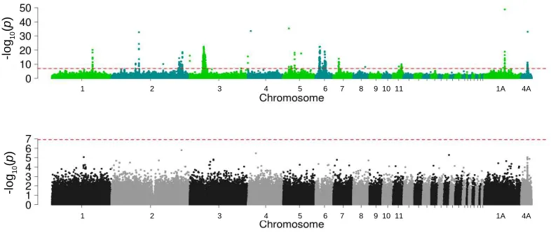
27
of feeders, suggesting that longer bills may have evolved in the UK as a response to supplementary
28
feeding.
Main Text: 30
To demonstrate evolutionary adaptation in wild populations we must identify phenotypes under
31
selection, understand the genetic basis of those phenotypes along with effects on fitness, and identify
32
potential drivers of selection. The best-known demonstrations of genes underlying evolution by natural
33
selection usually involve strong selection (‘hard sweeps’) on genetic variants, that may be recently
34
derived, with a major effect on variation in preselected phenotypes (1–3). However, most quantitative
35
phenotypes are polygenic (4) and for these traits selection is likely to act on many pre-existing genetic
36
variants of small effect (5). Detecting so-called polygenic selection is challenging because selection acts
37
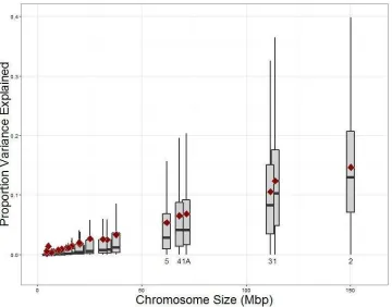
on multiple loci simultaneously and selection coefficients are likely to be small (6). Most attempts to
38
detect polygenic selection have focused on gene sets, rather than individual loci (e.g (7)). Furthermore,
39
even if population genomics analyses identify genes under selection, these analyses are rarely combined
40
with detailed ecological and behavioral data (8–10), and as a result linking all three components of the
41
genotype-phenotype-fitness continuum remains a challenge. In this study we combine fine-scale
42
ecological and genomic data to study adaptive evolution in the great tit (Parus major), a widespread and
43
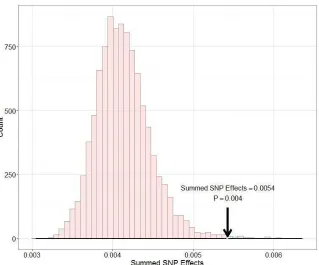
abundant passerine bird and well-known ecological model system (11) with excellent genomic resources
44
(12). To do so, we analyzed genomic variation within and among three long-term study populations from
45
the UK (Wytham, n = 949) and the Netherlands (Oosterhout, n = 254 and Veluwe, n = 1812; Fig. 1A).
46
47
After filtering (see methods), our dataset comprised 2322 great tits typed at 485,122 SNPs. Levels of
48
genetic diversity were high and linkage disequilibrium (LD) decayed rapidly within all three sample sites
49
(fig. S1). Admixture and principal component analyses (PCA) both suggest that genetic structure is low
50
(Fig. 1, B and C). These findings demonstrate a large effective population size and confirm high levels
51
of gene flow in the species (12, 13), making the long-term study populations well suited to studying
52
evolutionary adaptation.
53
To identify loci under divergent selection between the UK and Dutch populations, we ran a
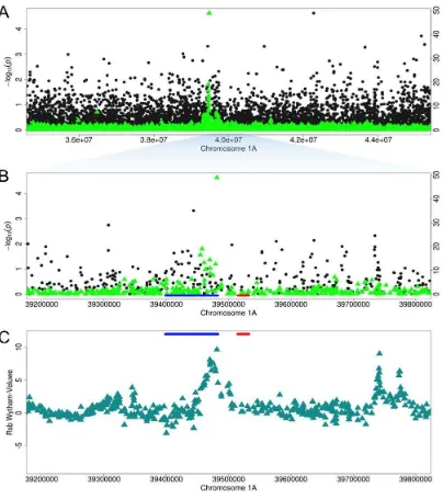
genome-55
wide association study using the first eigenvector from the PCA as a ‘phenotype’ (EigenGWAS (14)).
56
We identified highly significant outlier regions of the genome likely to be under divergent selection (fig.
57
2A, S2), which were supported by FST analyses (fig. S3). The majority of these outlier regions contained 58
candidate genes (e.g. COL4A5, SIX2, TRPS1, NELL1) involved in skeletal development and
59
morphogenesis (Fig. 2, A to C, table S1 and external database S1). Genes associated with the ontology
60
term “palate development” (GO:0060021; genes ALX4, BMPR1A, SATB2, INHBA, GLI3) were more
61
significantly overrepresented than any other GO term (Fig. 2C; Bonferroni-corrected p = 2.9 x 10⁻⁵;
62
external database S1). The strongest single-marker signal was found at the LRRIQ1 gene (table S1,
63
external database S1), where there was evidence of selection in Wytham, but not Veluwe (fig. S4).
64
LRRIQ1 is one of four genes located in the 240kb region associated with beak shape in Darwin’s finches
65
– arguably the best-known example of a trait undergoing adaptive evolution in the wild (15). Another
66
EigenGWAS peak contained VPS13B, a gene also associated with bill morphology in the Darwin’s finch
67
study, and with facial dysmorphism in humans (16).
68
69
Our genetic analyses therefore suggested bill morphology as a key trait involved in differentiation
70
between UK and Dutch great tit populations. Previously UK great tit populations have been characterized
71
as a different subspecies (P. major newtoni) compared to the rest of mainland Europe based on bill length,
72
but this classification is disputed (17)and it is unknown whether any bill length differences are adaptive
73
in this species. We examined the genetic architecture of bill length in the UK population, using two
74
complementary approaches. First, we fitted all SNPs simultaneously in a mixture model analysis (18),
75
and estimated that 3009 (95% credible interval 512-7163), or 0.8%, of the SNPs contributed to bill length
76
variation, suggesting that bill length is highly polygenic. Collectively these SNPs explained ~31% of the
77
phenotypic variation. The proportion of variance in bill length explained by each chromosome scaled
78
with its size, which is also consistent with a polygenic architecture (4) (fig. S5). Second, and consistent
with the mixture model analysis, we found multiple nominally significant SNPs in a GWAS on bill length
80
in Wytham, but even the most significant (p = 1.6 x 10⁻⁶) was not genome-wide significant after
81
accounting for multiple testing, perhaps as a consequence of small effect size and modest sample size.
82
Nonetheless, the SNPs were associated with bill length variation independently of overall body size
83
(Table S2). Using a sliding window approach, we found that the most significant GWAS regions largely
84
overlapped with the most significant regions in the EigenGWAS and FST analyses (Fig. 2, A and B, fig. 85
S3), suggesting that genes involved in bill length have been under divergent selection between
86
populations. We extracted SNPs from the most significant EigenGWAS peaks, calculated the summed
87
effect of those SNPs on bill length, and compared this against a null distribution generated by randomly
88
resampling the same number of SNPs and regions from across the genome. The regions under selection
89
explained a small amount of variation (0.54%) in bill length in the UK population, but this is more than
90
expected by chance (p = 0.004; fig. S6). Moreover, genomic prediction analysis using just the SNPs from
91
the EigenGWAS peaks showed that UK birds had breeding values for longer bills than birds from the
92
Netherlands (fig. S7), confirming that inter-population differences in bill length is at least partially
93
attributable to the loci that have been under recent selection.
94
95
The three genomic regions most notably associated with bill length variation and under likely divergent
96
selection (Fig. 2, A and B) all contained genes with annotations that make them candidates for
97
involvement in bill length. SOX6 is a transcription factor, and PTHrP a member of the parathyroid
98
hormone family; both are essential for bone development (19, 20). COL4A5 is a type IV collagen gene
99
best known for its association with Alport’s syndrome in humans (21), that has also been identified as a
100
candidate for craniofacial disorders (22). The ~400kb region of chromosome 4A containing the COL4A5
101
gene was the region most notably associated with bill length (4 of the 24 most significant SNPs in the
102
GWAS were in COL4A5; Table S2), and belongs to the top three regions under strongest divergent
103
selection between birds from the UK and Netherlands (Fig. 2, A and B). A closer inspection of the
individual SNPs within SOX6 and PTHrP reveals numerous SNPs that are nominally significantly
105
associated with bill length, but none as strongly as the COL4A5 SNPs; thus we focus on the COL4A5
106
locus hereafter. Patterns of genetic variation at COL4A5 reveal a clear signature of recent selection for
107
longer bills in the UK. First, the allele at the SNP that is most significantly associated with increased bill
108
length (hereafter ‘COL4A5-C’; Fig. 3D), is at higher frequency in the UK (0.54, bootstrap 95%
109
confidence intervals = 0.52-0.56) compared to the two Dutch populations (Veluwe: 0.28, CI = 0.27-0.29;
110
Oosterhout: 0.26, CI = 0.23-0.29). Second, extended haplotype homozygosity tests confirm that the
111
haplotype carrying the COL4A5-C allele extends further than alternative haplotypes within Wytham (Fig.
112
3, A to C). The COL4A5-C haplotype is longer and more abundant in Wytham compared to Veluwe, and
113
LD at this locus is much higher in Wytham, suggesting selection is UK-specific (fig. S8). Third, SNP
114
data from 15 European populations, including 3 UK populations, shows that the COL4A5-C allele is at
115
a higher frequency across the UK than across Europe (LGS et al. In Prep), consistent with selection on
116
this gene in the UK.
117
118
To further elucidate how natural selection has shaped variation in bill length across the two populations,
119
we tested how variation at the COL4A5 locus was related to annual reproductive success. We found
120
differences in the relationship between COL4A5 genotype and the number of chicks fledged between the
121
two populations (zero-inflated Poisson GLMM, interaction between genotype and population: n = 3076
122
breeding attempts from 1790 birds, estimate = -0.40 0.17, p = 0.016, Fig. 3E). The interaction was
123
significant because the associations between genotype and bill length in the two populations were in
124
opposite directions; in the UK, the number of copies of the ‘long-billed’ COL4A5-C allele was positively
125
associated with fledgling production (n = 868 breeding attempts from 516 birds, estimate = 0.23 0.11,
126
p = 0.046, Fig. 3E; fig. S9), whereas in the Dutch birds COL4A5-C was negatively, but not significantly,
127
associated with fewer fledglings (n = 2208 breeding attempts from 1274 birds, estimate = -0.16 0.10,
p = 0.093). The relationship between fledgling production and COL4A5 genotype did not arise because
129
long-billed genotype birds were more likely to produce offspring (binomial GLMM: n = 3076 breeding
130
attempts from 1790 birds, estimate = -0.20 0.17, p = 0.91); rather, when we only considered
131
“successful” breeding attempts in which at least one fledgling was produced, long-billed genotype birds
132
produced more fledglings (Poisson GLMM: n = 2690 breeding attempts from 1612 birds, estimate =
133
0.058 0.024, p = 0.018). Thus, we suggest that the COL4A5 allele associated with longer bills confers
134
a fitness advantage in the UK population.
135
136
To better understand the evolutionary consequences of selection for longer bills in the UK population,
137
we examined spatiotemporal variation in bill length. In museum samples from the UK and mainland
138
Europe, the UK individuals had considerably longer bills (n = 291, estimate = 0.40 0.06 mm, p = 5.2
139
x 10-12, R2 = 0.16, Fig. 4A), in accordance with a previous study (17). Using a 26-year dataset from live
140
birds in Wytham, we found that bill length has increased significantly over recent years (1982-2007; n =
141
2489, estimate = 0.004 0.001 mm per year, p = 0.0038, R2 of year effect = 0.004, Fig. 4B, table S3;
142
with tarsus length fitted as a covariate, the significant temporal increase in bill length remained
143
significant - n = 2485, estimate = 0.005 0.001 mm per year, p = 0.0001, R2 of year effect = 0.003). This
144
effect, though weak in terms of the variance explained, is not due to stochastic variation among years
145
(randomization test, P = 0.02, Supplementary Materials), and is equivalent to an evolutionary rate of
146
change of 0.0154 Haldanes; in a large review of phenotypic change in wild animal populations this rate
147
was exceeded in just 641 of 2420 estimates (23).
148
149
Selection on bill-length has been documented multiple times in birds, and is typically associated with
150
variation in food availability (24). No differences in the natural diet of great tits between the UK and
151
mainland Europe are known. In contrast, bird feeding by the public has been widespread in the UK since
the 19th Century; it is estimated it occurs in over 50% of gardens (25) and that the UK’s expenditure on
153
bird seed is twice that spent in the whole of mainland Europe (26). Great tits are particularly good at
154
exploiting bird feeders (27), and therefore we investigated whether supplementary feeding could have
155
been a driver of selection on bill length in UK great tits, similar to that proposed in UK blackcap (Sylvia
156
atricapilla) populations (28). Radio Frequency Identification (RFID) bird feeders throughout Wytham
157
recorded RFID-tagged great tit utilization of supplementary food over the course of three winters (29).
158
We found that COL4A5-C homozygotes displayed a higher propensity to use the feeders compared to
159
heterozygotes or short-billed homozygotes (n = 444, estimate = -0.17 0.08, p = 0.03, Fig. 3F). There
160
was some variation in the extent of this effect across winter seasons (Fig. S10), and the strength and
161
consistency of this effect, along with the mechanisms behind it, requires further investigation.
162
Encouragingly, however, a follow-up analysis using a more recent dataset gathered from high-resolution
163
RFID feeders (but on un-genotyped birds) showed a positive relationship between feeding propensity
164
and bill length (n = 1806 observations of 183 birds, estimate = 0.15 0.05, p = 0.004, Fig. S11).
165
166
Together, our results provide a detailed example of natural selection in a wild animal. Starting with a
167
bottom-up analysis of genomic data, and no-preselected phenotypes, we have demonstrated polygenic
168
adaptation by providing associations between loci that have responded to selection, fitness variation,
169
phenotypic variation, microevolutionary change and a possible driver of selection. Combining
large-170
scale genomic and ecological data in natural populations will significantly enhance our understanding of
171
both the mechanistic basis and evolutionary consequences of natural selection.
References and Notes:
1731. C. R. Linnen, E. P. Kingsley, J. D. Jensen, H. E. Hoekstra, On the origin and spread of an
174
adaptive allele in deer mice. Sci. (New York, NY). 325, 1095–1098 (2009).
175
2. S. Rost et al., Mutations in VKORC1 cause warfarin resistance and multiple coagulation factor
176
deficiency type 2. Nature. 427, 537–41 (2004).
177
3. S. Lamichhaney et al., A beak size locus in Darwin’s finches facilitated character displacement
178
during a drought. Science . 352 (2016).
179
4. J. Yang et al., Genome partitioning of genetic variation for complex traits using common SNPs.
180
Nat. Genet. 43, 519–525 (2011).
181
5. M. C. Turchin et al., Evidence of widespread selection on standing variation in Europe at
height-182
associated SNPs. Nat. Genet. 44, 1015–9 (2012).
183
6. J. K. Pritchard, J. K. Pickrell, G. Coop, The Genetics of Human Adaptation: Hard Sweeps, Soft
184
Sweeps, and Polygenic Adaptation. Curr. Biol. 20 (2010), , doi:10.1016/j.cub.2009.11.055.
185
7. J. J. Berg, G. Coop, A Population Genetic Signal of Polygenic Adaptation. PLoS Genet. 10,
186
e1004412 (2014).
187
8. R. D. H. Barrett, H. E. Hoekstra, Molecular spandrels: tests of adaptation at the genetic level.
188
Nat. Rev. Genet. 12, 767–780 (2011).
189
9. C. Pardo-Diaz, C. Salazar, C. D. Jiggins, Towards the identification of the loci of adaptive
190
evolution. Methods Ecol. Evol. 6, 445–464 (2015).
191
10. J. R. Stinchcombe, H. E. Hoekstra, Combining population genomics and quantitative genetics:
192
finding the genes underlying ecologically important traits. Heredity. 100, 158–170 (2007).
193
11. A. Gosler, The great tit (Hamlyn Species Guides, 1993).
194
12. V. Laine et al., Evolutionary signals of selection on cognition from the great tit genome and
195
methylome. Nat. Commun. (2016), doi:10.1038/ncomms10474.
13. N. E. M. Van Bers et al., The design and cross-population application of a genome-wide SNP
197
chip for the great tit Parus major. Mol. Ecol. Resour. 12, 753–770 (2012).
198
14. G.-B. Chen, S. H. Lee, Z.-X. Zhu, B. Benyamin, M. R. Robinson, EigenGWAS: finding loci
199
under selection through genome-wide association studies of eigenvectors in structured
200
populations. Heredity. 117, 51–61 (2016).
201
15. S. Lamichhaney et al., Evolution of Darwin’s finches and their beaks revealed by genome
202
sequencing. Nature. 518, 371–375 (2015).
203
16. I. Balikova et al., Deletions in the VPS13B ( COH1 ) gene as a cause of Cohen syndrome. Hum.
204
Mutat. 30, E845–E854 (2009).
205
17. A. G. Gosler, A comment on the validity of the British Great Tit Parus major newtoni. Bull. Br.
206
Ornithol. Club. 119, 47–55 (1999).
207
18. G. Moser et al., Simultaneous Discovery, Estimation and Prediction Analysis of Complex Traits
208
Using a Bayesian Mixture Model. PLOS Genet. 11, e1004969 (2015).
209
19. N. Hagiwara, Sox6, jack of all trades: A versatile regulatory protein in vertebrate development.
210
Dev. Dyn. 240, 1311–1321 (2011).
211
20. H. M. Kronenberg, PTHrP and Skeletal Development. Ann. N. Y. Acad. Sci. 1068, 1–13 (2006).
212
21. D. F. Barker et al., Identification of mutations in the COL4A5 collagen gene in Alport
213
syndrome. Science. 248, 1224–1227 (1990).
214
22. J. J. Jonsson et al., Alport syndrome, mental retardation, midface hypoplasia, and elliptocytosis:
215
a new X linked contiguous gene deletion syndrome? J Med Genet. 35, 273–278 (1998).
216
23. A. P. Hendry, T. J. Farrugia, M. T. Kinnison, Human influences on rates of phenotypic change
217
in wild animal populations. Mol. Ecol. 17, 20–29 (2008).
218
24. P. R. Grant, B. R. Grant, Unpredictable evolution in a 30-year study of Darwin’s finches.
219
Science. 296, 707–711 (2002).
220
25. M. E. Orros, M. D. E. Fellowes, Wild Bird Feeding in an Urban Area: Intensity, Economics and
Numbers of Individuals Supported. Acta Ornithol. 50, 43–58 (2015).
222
26. D. N. Jones, S. James Reynolds, Feeding birds in our towns and cities: a global research
223
opportunity. J. Avian Biol. 39, 265–271 (2008).
224
27. P. Tryjanowski et al., Who started first? Bird species visiting novel birdfeeders. Sci. Rep. 5,
225
11858 (2015).
226
28. G. Rolshausen, G. Segelbacher, K. A. Hobson, H. M. Schaefer, Contemporary Evolution of
227
Reproductive Isolation and Phenotypic Divergence in Sympatry along a Migratory Divide. Curr.
228
Biol. 19, 2097–2101 (2009).
229
29. R. A. Crates et al., Individual variation in winter supplementary food consumption and its
230
consequences for reproduction in wild birds. J. Avian Biol. (2016), doi:10.1111/jav.00936.
231
30. S. Purcell et al., PLINK: A Tool Set for Whole-Genome Association and Population-Based
232
Linkage Analyses. Am. J. Hum. Genet. 81, 559–575 (2007).
233
31. J. Yang, S. H. Lee, M. E. Goddard, P. M. Visscher, GCTA: A Tool for Genome-wide Complex
234
Trait Analysis. Am. J. Hum. Genet. 88, 76–82 (2011).
235
32. D. H. Alexander, J. Novembre, K. Lange, Fast model-based estimation of ancestry in unrelated
236
individuals. Genome Res. 19, 1655–1664 (2009).
237
33. R Development Core Team, R. D. C. Team, Ed., R: A Language and Environment for Statistical
238
Computing. R Found. Stat. Comput. (2011), , doi:10.1007/978-3-540-74686-7.
239
34. P. C. Sabeti et al., Detecting recent positive selection in the human genome from haplotype
240
structure. Nature. 419, 832–837 (2002).
241
35. O. Delaneau, J. Marchini, J.-F. Zagury, A linear complexity phasing method for thousands of
242
genomes. Nat. Methods. 9, 179–181 (2011).
243
36. M. Gautier, R. Vitalis, rehh: an R package to detect footprints of selection in genome-wide SNP
244
data from haplotype structure. Bioinformatics. 28, 1176–1177 (2012).
245
37. K. Tang, K. R. Thornton, M. Stoneking, A new approach for using genome scans to detect
recent positive selection in the human genome. PLoS Biol. 5, 1587–1602 (2007).
247
38. G. Bindea et al., ClueGO: a Cytoscape plug-in to decipher functionally grouped gene ontology
248
and pathway annotation networks. Bioinformatics. 25, 1091–1093 (2009).
249
39. A. G. Gosler, Pattern and process in the bill morphology of the Great Tit Parus major. Ibis
250
(Lond. 1859). 129, 451–476 (2008).
251
40. J. D. Hadfield, MCMC methods for multi-response generalized linear mixed models: the
252
MCMCglmm R package. J. Stat. Softw. 33, 1–22 (2010).
253
41. Y. S. Aulchenko, S. Ripke, A. Isaacs, C. M. van Duijn, GenABEL: an R library for
genome-254
wide association analysis. Bioinformatics. 23, 1294–6 (2007).
255
42. Y. S. Aulchenko, D.-J. de Koning, C. Haley, Genomewide Rapid Association Using Mixed
256
Model and Regression: A Fast and Simple Method For Genomewide Pedigree-Based
257
Quantitative Trait Loci Association Analysis. Genetics. 177 (2007).
258
43. S. Bouwhuis et al., Great tits growing old: selective disappearance and the partitioning of
259
senescence to stages within the breeding cycle. Proc. R. Soc. B Biol. Sci. 276, 2769–77 (2009).
260
44. M. Erbe et al., Improving accuracy of genomic predictions within and between dairy cattle
261
breeds with imputed high-density single nucleotide polymorphism panels. J. Dairy Sci. 95,
262
4114–4129 (2012).
263
264
Acknowledgements: We thank the many researchers who collected material and data for the Wytham 265
study, Louis Vernooij, Piet de Goede and Henri Bouwmeester for fieldwork on the Dutch populations
266
and Christa Mateman for lab assistance. The Natural History Museums in London (NHM) and Oxford
267
(OUMNH) kindly granted us access to great tit specimens. R. Butlin, N. Nadeau and P. Nosil provided
268
helpful comments on the manuscript. This work was supported by grants from the ERC (339092 to MEV,
269
250164 to BCS and 202487 to JS), BBSRC (BB/N011759/1 to LGS) and NERC (NE/J012599/1 to JS).
270
Author contributions: M.B., L.G.S., M.A.M.G., B.C.S., M.E.V. and J.S. designed the study. M.B., L.G.S.
271
and J.S. analyzed the genomic data for signatures of selection. V.N.L, P.G. and J.S. analyzed estimated
272
trait genetic architectures. V.N.L performed gene ontology analyses. A.G.G., K.M., J.P. and I.V.
273
measured and analyzed bills. L.G.S., E.F.C and J.A.F. collected and analyzed bird feeding station data.
274
E.F.C, J.A.F, A.G.G., K.vO., B.C.S and M.E.V. coordinated and collected ecological data and DNA
samples. M.A.M.G., K vO., M.E.V. and J.S. coordinated collection of SNP data. M.B., L.G.S, V.N.L.
276
and J.S. cleaned and QC checked SNP data. M.B., L.G.S and J.S. wrote the manuscript with input from
277
all other authors. The data described in the paper are archived on Dryad with accession number XXX.
Supplementary Materials 279
Materials and Methods
280
Supplementary Text
281
Tables S1 – S3
282
Fig S1 – S9
283
Caption for database S1
284
References (30–44)
285
286
Fig. 1. Population structure of Western European great tits. (A) Worldwide distribution of P. major 287
and sampling locations in Wytham ( ) Oosterhout ( ) and Veluwe ( ). (B) Principal component
288
analysis of genotype data. (C) ADMIXTURE plot with K=3, which is both the most likely number of
289
clusters and the number of geographically distinct sampling sites. Levels of genetic structure are low
290
(FST Veluwe-Wytham = 0.006, and FST Veluwe-Oosterhout = 0.003). 291
292
Fig. 2. Differentiation and regions under selection across two great tit populations. (A) Upper panel: 293
EigenGWAS on PC1 across all autosomes, averaged over 200kb sliding windows. Genes surrounding or
294
covering peaks are indicated. Gene names highlighted in bold green belong to the most significant
GO-295
term 'palate development'. Lower panel: GWAS for bill length in the UK population, averaged over
296
200kb sliding windows. Color-highlighted regions indicate peaks found in both the GWAS and
297
EigenGWAS analyses. (B) EigenGWAS p-values in relation to bill length GWAS p-values averaged
298
over 200kb windows. Color-highlighted points correspond with the highlighted regions in (A). (C) Gene
299
Ontology network of genes in or surrounding the EigenGWAS peaks. Size of circles indicates
300
significance and line thickness indicates proportion of shared genes.
301
Fig. 3. COL4A5 locus on chromosome 4A. (A) 2Mb zoom of EigenGWAS (green triangles) and GWAS 303
(black circles) p-values at the COL4A5 region (highlighted blue in Fig. 2A). Red horizontal bars indicate
304
gene locations (B and C) Bifurcation diagram for haplotypes in Wytham, starting from the two alleles at
305
the most significant GWAS SNP. Note the extended haplotype at the COL4A5-C-allele in (C), relative
306
to the shorter haplotypes at the COL4A5-T allele in (B), consistent with a recent selective sweep around
307
the COL4A5-C allele in the UK. (D) Bill length and COL4A5 genotype; the C allele is associated with
308
longer bills (R2 = 0.035). (E) The COL4A5-C allele is associated with greater annual fledgling production
309
in the UK population (R2 = 0.015). (F) COL4A5-C allele birds display greater winter feeding site activity
310
– the y axis is log10 transformed cumulative activity records (R2 = 0.01). Lines and shaded areas in d-f 311
are fitted values and 95% confidence limits from general(ized) linear models (full data are plotted in Figs
312
S8 and S9).
313
314
Fig. 4. Spatiotemporal variation in bill length. (A) Bill lengths of museum samples from the UK and 315
mainland Europe.(B) Temporal variation in bill length in the Wytham population plotting annual
316
means with standard error from 1982-2007. Line and (narrow) shaded area in b are fitted values and
317
95% confidence limits from a linear regression (R2 = 0.004); note different scales on axes in A and B.
1
Supplementary Materials for
Recent natural selection causes adaptive evolution of an avian polygenic
trait
Mirte Bosse, Lewis G. Spurgin, Veronika N. Laine, Ella F. Cole, Josh A. Firth, Phillip Gienapp, Andrew G. Gosler, Keith McMahon, Jocelyn Poissant, Irene Verhagen, Martien
A. M. Groenen, Kees van Oers, Ben C. Sheldon, Marcel E. Visser, Jon Slate
correspondence to: [email protected]
This PDF file includes:
Materials and Methods Supplementary Text Figs. S1 to S11 Tables S1 to S3
Caption for database S1
Other Supplementary Materials for this manuscript includes the following:
2
Materials and Methods
Sampling
Sample sites: Samples were collected from three distinct forest areas in Western Europe (Fig. 1A): Wytham (UK); Oosterhout (Netherlands) and Veluwe (Netherlands). All three sample locations are long-term study sites for great tit research.
Sampling: Blood was collected from a total of 949 specimens in Wytham, 254 in Oosterhout and 2058 in Veluwe. Blood samples were stored in either 1 ml Cell Lysis Solution (Gentra Puregene Kit, Qiagen, USA) or Queen’s buffer. DNA was extracted from these samples by using the FavorPrep 96-Well Genomic DNA Extraction Kit (Favorgen Biotech corp.). DNA quality and DNA concentration were measured on a Nanodrop 2000 (Thermo Scientific).
Genotyping and filtering
Great tits were genotyped using a custom made Affymetrix® great tit 650K SNP chip at Edinburgh Genomics (Edinburgh, United Kingdom).
Netherlands birds: A total of 2066 female great tits were genotyped and passed quality
control. SNP calling was done following the Affymetrix® best practices steps in Axiom® Genotyping Solution Data Analysis Guide by using the Affymetrix® Genotyping console 4.2.0.26. Eight individuals with dish quality control value of <0.82 were discarded. SNP quality control was done by using Affymetrix Power Tools software package 1.16.1 and the functions Ps_Metrics and Ps_Classification. The recommended SNP group consisted of 505,604 SNPs while 105 366 SNPs were discarded because their call rate was below the threshold (<0.97), because they were “off-target” variants or because they belonged to the “other” group of suboptimal SNPs. In addition to the SNPs that did not pass the Ps_Metrics and Ps_Classification steps, an additional 388 SNPs were removed because they were duplicates or the genomic position was missing. Altogether 505,216 SNPs passed initial quality control.
UK birds: SNP calling was performed using the Affymetrix Axiom Analysis Suite
1.1.0.616, the successor of the Genotyping Console described above. The same quality control thresholds were used as for the Netherlands birds; samples with dish QC < 0.82 or call rates <0.95 were discarded, as were SNPs with call rates <0.97. A total of 1,846 samples typed at 498,036 SNPs were retained for analysis. 996 of the samples, which included replicates for error checking, were from Wytham Woods – the remainder were from other populations that are not the focus of this study. Replicated error samples suggested a per SNP genotyping error rate of 0.004 (among samples with call rates >0.98, the error rate was 0.002).
3 Genetic diversity analyses
Pairwise relatedness between individuals and linkage disequilibrium for all SNP pairs up to 200kb apart within populations were calculated per population in PLINK v1.90b3x (30). Based on a visual inspection of the distribution of relatedness values, we removed individuals from pairs with relatedness > 0.4 for all further analyses, leaving us with 2322 birds from the three sample sites. Pairwise FST between the three populations was
calculated in PLINK. The filtered dataset was LD-pruned in PLINK (Variance Inflation Factor>2) which resulted in 375,846 SNPs. Principal component analysis was performed on the filtered and pruned dataset using the GCTA package (31). A small percentage of birds from all three populations displayed atypical clustering based on SNPs on chromosome 1A, possibly representing a large inversion (data not shown). Therefore, chromosome 1A, as well as chromosome Z and the small linkage groups were excluded from PCA analysis. Admixture analysis was performed on the filtered and pruned data using the software package ADMIXTURE v1.23 (32) with K ranging from 2 to 5.
Selection analyses
The populations were screened for between-population signatures of selection with two distinct measures. The EigenGWAS package (14) was used to apply a GWAS framework to the first two eigenvectors of the principal component analysis. The main rationale for using EigenGWAS over an FST outlier locus test, is that it is more flexible. There is no need to predefine populations (although clearly we can do so here), and the analysis accounts for population stratification (e.g. due to the presence of relatives). The EigenGWAS is quick and easy to implement, and the results are conceptually comparable to a standard GWAS (i.e. where markers are used to identify genomic regions that explain phenotypic variation). Chromosome 1A was excluded from the PCA but included in the EigenGWAS, due to the potential inversion (see above). As a comparison to the EigenGWAS test, we also calculated single-marker pairwise FST using PLINK, with
predefined clusters according to sampling sites. FST and EigenGWAS results were almost
identical (fig. S2) We used Pearson's product-moment correlation in R(33) to test for correlation between the EigenGWAS corrected p-value and FST between Veluwe and
Wytham.
4 Gene ontology analyses
Regions under selection were tested for an overrepresentation of genes belonging to specific gene ontology terms. Candidate genes for all EigenGWAS peaks containing markers with p-value <10-9 were extracted if they were 1) overlapping the most significant marker; 2) surrounding the peaks if no overlapping gene was present. Since the peaks are relatively narrow, mostly only one or two genes overlapped the peaks (see Additional Data table S1). Candidate genes were extracted from the great tit reference annotation (NCBI Parus major Annotation Release 100).
Functional relatedness of Gene Ontology (GO) terms was performed using the Cytoscape plugin ClueGO 2.2.4 (38). ClueGO constructs and compares networks of functionally related GO terms with kappa statistics. A two-sided hypergeometric test (enrichment/depletion) was applied with GO term fusion, network specificity was set to ‘medium’ and false discovery correction was carried out using the Bonferroni step down method. We used both human (8.3.2016) and chicken gene ontologies (9.3.2016) for comparison. With human gene ontologies we detected 16 functional groups of GO terms (Supplementary Data). These groups were mainly involved in functions concerning palate development, positive regulation of osteoblast differentiation and mesoderm formation. When using the chicken orthologues the results were comparable, but with more significant GO groups (26 groups) and with higher P values (Supplementary Data). This is because the chicken genes were not as well GO-annotated as the human genes.
Genetic architecture of bill length
To understand the genetic architecture of bill length we used two fundamentally different approaches. First, a genome-wide association study (GWAS) was performed to test for associations between SNP genotypes and the focal trait, fitting one SNP at a time. However, a GWAS on a dataset of this magnitude is unlikely to detect genome-wide significant loci, unless there are major effect loci affecting the trait. Second, to further understand the architecture of bill length we ran analyses that fitted all SNPs in one model; hereafter we call this the ‘BayesR’ analysis after the method (39) and software (18) used to perform the analysis. BayesR can simultaneously estimate effect sizes of individual SNPs, making it possible to estimate a trait’s heritability, partition variation across the genome, and perform genomic prediction. There were several rationales for performing this analysis. First, we could investigate whether bill length is a polygenic trait. Second, we could estimate the effects of all SNPs on bill length in one model, and then use these estimated effects to ask whether regions under selection disproportionately contribute to bill length variation. Third, we could perform genomic prediction to test the extent to which the differences in bill length between the UK and Netherlands populations are caused by the SNPs under selection.
GWAS analysis
5 effects in the model included individual identity, year of birth and age category (used to distinguish recent fledglings, adult birds of different ages and birds of unknown age). Sex was fitted as a fixed effect. The GenABEL functions polygenic and grammar were used to run a GWAS that uses genomewide realized relatedness to control for population structure caused by the presence of related individuals (41). To test whether the effect was caused by correlated traits, we ran the same analysis on bill length with bill depth and tarsus lengths for the same birds included as covariates in the model.
BayesR analysis
The BayesR analysis was performed using default parameters - SNP effects were assumed to be drawn from a mixture of 4 normal distributions, with SNPs having a variance of 0, 0.0001, 0.001 or 0.01 of the genetic variation. MCMC chains were run for 50,000 samples, with a 20,000 sample burn-in, followed by every 10th sample being used. This gave a total of 3000 used samples. For each sample the number of SNPs in the non-zero effect size distributions were counted. The mean and 95% confidence intervals for the number of SNPs contributing to trait variance was determined from the 3000 samples. SNP effect sizes (ß) were reported in terms of the phenotypic change caused by an allelic substitution from one allele to another. The proportion of trait variation explained by each SNP was then estimated as VSNP = 2 * ß2 * p * (1-p) where p is the frequency of the minor allele.
BayesR also returns an estimate of trait heritability and the number of typed SNPs that contribute to trait variation (or, more likely, tag causal variants because they are in LD with them).
If a trait is polygenic, then the proportion of variance explained by each chromosome should scale with chromosome size (4). We tested this by estimating the proportion of variance explained by each chromosome. This was done by summing, across chromosomes, the effect sizes of all SNPs from the non-zero distributions, and estimating the proportion of additive genetic variance explained by each chromosome. The process was performed for each of the 3000 samples, from the MCMC chain.
Do SNPs under selection explain bill length variation?
The GO term analysis suggested that the EigenGWAS SNPs under selection (‘candidate SNPs’) should affect craniofacial traits, and in particular bill length. To test for an overlap between the most significant EigenGWAS regions and peaks in the GWAS on bill length, we used a sliding window approach, averaging the signal from all markers within 200kb windows sliding in steps of 50kb along the genome. The rationale for this is that due to low LD between sites, allele frequency differences and SNPs imperfectly tagging sites under selection, single markers in a significant region do not necessarily result in a high signal for both EigenGWAS and GWAS statistics, even when the underlying region is the same. Sliding window based approaches are therefore more powerful for identifying regions that overlap between the EigenGWAS and GWAS.
6 BayesR estimates of SNP effect sizes. We first defined which SNPs were included in the EigenGWAS peaks. For all eigenGWAS peaks (peaks where P <10-9), the core SNPs with the lowest EigenGWAS p-values were extracted (17 regions in total, see Table S1). Starting from these core SNPs, flanking markers were included until 10 consecutive markers did not include 1 marker with an EigenGWAS signal within the top 1% of most significant EigenGWAS p-values. This way, 16 genomic candidate regions were extracted with a total number of 1530 SNPs. The randomization test sampled the same number of SNPs, in the same number of regions, at randomly chosen positions in the genome, and then summed the effects of those SNPs on bill length variation. By sampling the genome 1000 times, we were able to generate a null distribution for the amount of bill length variation explained by 1530 SNPs. We tested our observed data from the eigenGWAS candidates against this null distribution.
Genomic prediction
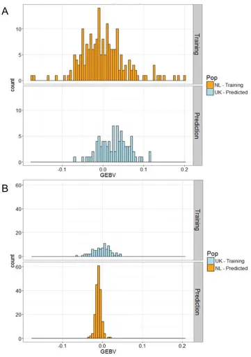
We predicted that the SNPs that were under selection in the eigenGWAS analysis would cause the UK birds to have longer bills than NL birds. Genomic prediction uses estimates of SNP effects in one population (a ‘training’ population), to then predict genomic estimated breeding values (GEBVs) in a second population that has been genotyped at the same SNPs (the ‘test’ population). Note that the phenotypes in the ‘test’ population are not used to estimate breeding values in that population. Therefore, inter-population differences in GEBVs should be attributable to genetic differences between the two populations. Genomic prediction analyses were performed using the –predict command in BayesR. The test was done reciprocally, using the eigenGWAS candidate SNP. First, SNP effects were estimated in 87 UK birds and used to predict genomic estimated breeding values (GEBVs) in 194 genotyped Netherlands birds (fig. S6). Next, the SNP effects were estimated from the 194 Netherlands birds and these estimates were used to predict GEBVs in the 87 UK birds. The sample sizes are small, making it hard to reliably predict variation in breeding values within a population, but because inter-population variation is typically greater than intra-population variation, the analysis should be capable of detecting population differences. Comparisons between the GEBVs of each population were performed by two sample t-tests with Welch’s correction for unequal variances.
Spatiotemporal trends in bill length
We investigated spatiotemporal variation in bill length, using both 291 museum specimens from across Europe and temporal data available from Wytham. The museum specimens and Wytham data were each measured by a single measurer (KM and AGG, respectively), following a standardized methodology (42). Using the museum specimens, we tested for a difference in bill length between UK and mainland European samples using a general linear model, with bill length as the response variable, and population ID, year of collection, age and sex as explanatory variables.
7 when aged 1 year old. A small number of birds were measured more than once, and for these individuals a mean measurement was taken. Sex and Year of Birth were fitted as main effects in a linear model. One bird had an exceptionally long bill, but was retained in the model. The results are robust to its exclusion. We confirmed that temporal changes in bill length were not due to trends in overall body size, by rerunning the models with tarsus length, an indicator of overall body size, fitted as a covariate. We measured the rate of change in bill length in Haldanes, using the framework described in Hendry et al (23). The difference in bill length between the start and end of the time series was divided by the product of the standard deviation of bill length and the number of generations that had elapsed during the time series. Thus, the rate of change is measured in standard deviations per generation. Bill length was natural log-transformed prior to estimation. Generation length was assumed to be 1.81 years, following Bouwhuis et al. (43). The difference in bill length between the UK and NL populations is approximately 1.27 standard deviations.
A larger dataset contained 9980 records collected on 5145 birds. Modelling this data was more complex as birds were of different ages and measurements were taken at different times of year - bill length is known to vary seasonally (39). Therefore, a linear mixed effects model implemented in MCMCglmm (44) was fitted. Fixed effects were year of birth (mean-centered) and sex, while random effects included ID, month of measurement, age category at measurement, and whether or not the bird was an immigrant.
To check that our observed change in bill length over time (see results) could not come about due to stochastic, yet highly significant, year-to-year variation, instead of a temporal trend, we performed a simple simulation. We randomly re-assigned cohort years, while keeping the same individuals “together” in cohorts. Using such an approach, we expect high levels of year-to-year variation, but this variation should be random with respect to variation over time. We generated 500 randomised datasets in this way, and performed a linear model of bill length against (randomised) birth year in each dataset.
COL4A5 and reproductive success
8 Visits to supplementary feeding sites in Wytham
We tested how variation at COL4A5 was related to the propensity for individuals to use supplementary food resources. Since 2007, all captured great tits have been fitted with Radio Frequency Identification (RFID) tags for studies of social behavior (29). These tags allow the automated recording of their visits to bird feeders fitted with RFID antennae and filled with sunflower seeds (hereafter ‘RFID feeders’). We used data over three winters (2007-2010), for which we had reasonable sample sizes of genotyped birds (N = 167 for 2007-2008, 142 for 2008-2009 and 135 for 2009-2010).
The RFID feeding locations comprised of a stratified grid of 67 locations throughout Wytham Woods, but whether or not an RFID feeder was present at each location at any given time depended on the temporal feeding regime. Through these winters, 16 of the 67 locations contained RFID feeders at any one time. In winters beginning 2007 and 2008, RFID feeders were rotated every 4 days in a structured random design so that each of the eight similarly sized sections of Wytham contained two feeders. In 2009, rotations took place on a 7-day basis. In this way, each of the 67 grid locations contained an RFID feeder twice a month in the winters beginning in 2007 and 2008, and once a month (but for a longer period) in 2009. The RFID feeders utilized over these periods scanned for RFID tags 16 times per second, and observations showed that >99% of visits by RFID-tagged birds to the feeder were successfully recorded. During the winters 2007-2010, the RFID feeders automatically binned all records of the same bird into 15s time intervals i.e. for each minute, only one record of each bird would be stored in the time intervals of 0-14s, 15-29s, 30-44s and 45-59s of that minute. More recently (2012 onwards), higher resolution RFID feeders have been deployed which store up to two records by each bird each second. This high resolution data has allowed fine-scale estimates of actual seed consumption to be determined (29). However, upon binning the high resolution data into 15s time bins, we found that the raw number of records from this procedure correlates strongly with the actual estimated number of seeds consumed (r = 0.98). Therefore, bird feeder activity recorded in this way is likely to be an ecologically relevant measure of supplementary food usage.
From the RFID feeder records, we then calculated three measures of individual activity on bird feeders for each of the winter seasons (2007-08, 2008-09, 2009-10) separately. First, we calculated the mean number of records each bird showed per day it was recorded. Second, we calculated the number of days each bird was recorded utilizing the feeders. Finally, we summed the total number of records for each bird over the winter season. We then ran GLMMs with a poisson error distribution, using each of these measures as the response variable. Genotype was modeled as a continuous variable (0 = CC, 1 = CT and 2 = TT) to reduce the degrees of freedom. Sex, month (ordinal from start of winter, with a quadratic term fitted) and season were also included as fixed effects, individual ID was fitted as a random effect, and an observation-level random effect was fitted to the GLMMs to account for overdispersion.
10
Supplementary Figures
Fig. S1. Linkage disequilibrium (LD) decay in the three great tit populations. Distance
[image:26.612.101.564.114.485.2]11
Fig. S2. Single marker (-log10) p-value for EigenGWAS on PC1 (green and blue dots, above) and GWAS on bill length (gray tones, below). Genomewide significance thresholds were generated by performing Bonferroni correction on the effective number of independent tests, estimated with the Genetic Type 1 Error Calculator (downloadable at
[image:27.612.98.491.90.258.2]12
Fig. S3. FST and EigenGWAS analyses reveal identical patrterns of divergent selection, including at genes associated with bill length. A 200kb sliding window FST and B 200kb
sliding window p values from a GWAS of bill length. Shaded regions correspond to the same shaded regions in figure 2 in the main text. C FST values and GWAS p values are
correlated, with three shaded regions showing high levels of structure and associations with bill length. D The reason the effects are identical is that FST and EigenGWAS (PC1)
[image:28.612.98.517.71.430.2]13
Fig. S4. (A and B) Zoom of the LRRIQ1 and ALX1 region on Chromosome 1A. Black dots
represent bill length GWAS (-log10) p-values (left y-axis) and bright green triangles
represent EigenGWAS (-log10) p-values (right y-axis). (C) Rsb across the same region.
[image:29.612.112.516.94.549.2]14
Fig. S5. The proportion of additive genetic variance of bill length explained by a
[image:30.612.95.455.86.368.2]15
Fig. S6. Randomization test for summed SNP effect on bill length. Distribution of summed
16
Fig. S7. Genomic estimated breeding values (GEBVs) for bill length. (A) GEBVs for
Wytham using candidate SNP effect sizes, predicted from Veluwe as a training population. Wytham GEBVs are greater than Veluwe GEBVs (t = 4.897, d.f. = 246.14, p = 1.8 x 10
-6) (B) GEBVs for Veluwe using candidate SNPs effect sizes, predicted from Wytham as a
[image:32.612.105.466.88.602.2]17
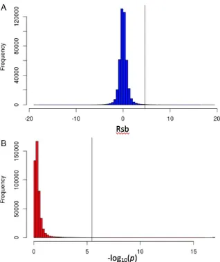
Fig. S8. Distribution of the Rsb statistic (A) and p-values (B) for all SNPs. Rsb values
[image:33.612.103.421.91.469.2]18
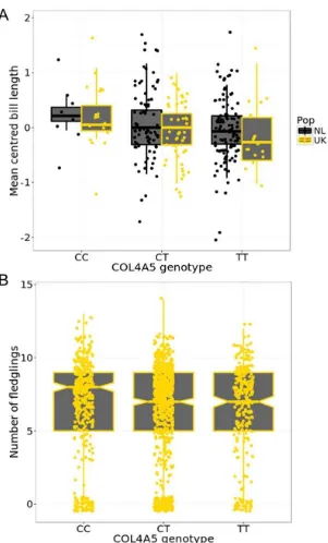
Fig. S9. (A) Mean-centered bill length in relation to genotype in the UK and Dutch
[image:34.612.116.417.83.581.2]19
Fig. S10. Activity at feeding stations and COL4A5 genotype. (A). Genotype and mean
[image:35.612.92.516.71.627.2]21
Fig. S11. Activity at feeding stations (number of activity records per day; see methods)
[image:37.612.95.510.76.444.2]21
Table S1. List of most significant markers in EigenGWAS peaks. Regions included in the genomic prediction and BayesR analysis
surrounding the top markers are indicated, and candidate genes for those regions are listed. Start and Stop refer to the locations of the entire EigenGWAS peaks, not gene locations. Numbers in brackets indicate total number of genes in the region.
SNP CHR BP Freq Pgc Start Stop Candidate
AX-100016177 1 77,696,913 0.216 7.45E-21 77,663,865 77,762,204 HEPHL1
AX-100056392 2 52,689,192 0.132 2.08E-33 52,658,347 52,748,564 GLI3
AX-100827868 2 129,918,616 0.209 4.88E-15 129,804,789 129,938,703 VPS13B
AX-100550602 2 136,196,505 0.205 2.47E-19 136,026,079 136,211,161 TRPS1
AX-100957595 3 25,770,657 0.252 5.91E-17 25,579,744 26,000,833 SRBD1/ SIX2/ SIX3
AX-100923788 3 26,810,200 0.19 2.23E-22 26,722,719 28,252,952 SOCS5 (10)
AX-100516656 3 29,160,891 0.368 1.84E-17 28,442,822 31,002,208 DAAM2 (39)
AX-100959055 5 10,662,578 0.122 3.90E-36 10,449,814 11,190,618 SLC17A6/ ANO5/
LOC107206397/ NELL1
AX-100690978 5 21,629,221 0.297 7.36E-19 21,567,485 21,675,638 ALX4 CD82
AX-100474351 5 34,236,075 0.229 2.33E-18 34,222,212 34,237,466 LOC107205269/
LOC107205369
AX-100471694 6 7,561,954 0.218 6.29E-23 6,927,592 8,874,881 LDB3/BMPR1A (19)
AX-100402843 6 8,342,760 0.218 3.52E-23 6,927,592 8,874,881 CDHR1/NRG3 (19)
AX-100289034 6 17,406,899 0.223 8.44E-20 17,383,685 18,150,016 SHD24B (6)
AX-100326794 7 10,164,383 0.15 1.35E-14 10,143,016 10,241,782 SATB2/ LOC107207327
AX-100350351 11 16,307,406 0.282 9.72E-11 16,245,749 16,358,113 VAT1L/ ADAMTS18
AX-100642371 1A 39,481,264 0.205 1.49E-49 39,454,093 39,504,418 LRRIQ1
22
Table S2. List of most significant markers in the GWAS for bill length. The P value is corrected using a lambda inflation factor. The
Last three columns report the results with bill depth and tarsus length fitted as covariates. Effect size and SE are the effect of an allelic substitution in mm. Where SNPs are within genes, the gene name is reported. SNPs significant at 5x10⁻⁵ are reported.
SNP CHR Position P Effect SE Gene P Effect SE
Without covariates
Tarsus length & bill depth as covariates
AX-100161487 2 134,506,393 1.60E-06 0.361 0.075 3.84E-07 0.382 0.075
AX-100162335 4 15,291,962 3.40E-06 0.546 0.118 4.56E-07 0.587 0.116
AX-100219258 18 9,840,163 5.20E-06 0.441 0.097 MYOCD 4.04E-06 0.441 0.096
AX-100772359 1 60,802,871 8.70E-06 -0.392 0.088 LRCH1 3.02E-05 -0.375 0.090
AX-100866146 4A 11,968,430 8.90E-06 -0.387 0.087 COL4A5 1.91E-05 -0.375 0.088
AX-100415796 4A 15,974,127 1.33E-05 -0.884 0.203 CMC4 2.25E-05 -0.866 0.204
AX-100790037 4A 11,948,539 1.35E-05 0.376 0.086 COL4A5 3.28E-05 0.361 0.087
AX-100763101 3 45,380,348 1.55E-05 -0.343 0.079 1.11E-05 -0.348 0.079
AX-100983338 4A 11,971,129 1.55E-05 -0.374 0.086 COL4A5 2.88E-05 -0.363 0.087
AX-100427980 7 6,552,913 1.68E-05 -0.541 0.126 1.28E-05 -0.550 0.126
AX-100121530 3 45,463,659 1.81E-05 -0.834 0.194 2.91E-05 -0.809 0.194
AX-100317140 8 29,545,515 1.97E-05 -0.330 0.077 CACHD1 5.92E-05 -0.312 0.078
AX-100344380 2 91,033,979 1.97E-05 0.475 0.111 ERP44 4.21E-05 0.455 0.111
AX-100551558 2 9,029,184 2.10E-05 -0.488 0.115 PTPRN2 2.45E-05 -0.484 0.115
AX-100268275 1A 42,273,688 2.32E-05 -0.565 0.134 EEA1 4.04E-06 -0.616 0.134
AX-100043541 3 39,378,229 2.71E-05 -0.400 0.095 2.56E-05 -0.401 0.095
AX-100395747 2 35,488,576 3.34E-05 0.363 0.088 TBC1D5 1.33E-05 0.381 0.088
AX-100354346 2 15,476,538 3.47E-05 1.136 0.274 MPP7 1.49E-05 1.198 0.277
AX-100510816 2 15,509,848 3.47E-05 1.136 0.274 MPP7 1.49E-05 1.198 0.277
AX-100855556 2 15,493,743 3.47E-05 1.136 0.274 MPP7 1.49E-05 1.198 0.277
AX-100537714 4A 11,971,623 3.59E-05 0.343 0.083 COL4A5 7.24E-05 0.332 0.084
AX-100928290 1A 26,968,602 3.89E-05 -0.352 0.086 CNTN1 4.17E-05 -0.349 0.085
AX-100605138 1A 52,409,448 4.56E-05 -0.470 0.115 TXNRD1 1.54E-04 -0.444 0.116
23
Table S3: Summary of general linear mixed model of temporal trends in bill length in
Wytham dataset (9980 measurements taken on 5145 birds between 1976 and 2010). Repeatability of bill length is 0.62 (95% CI = 0.60-0.64).
Random Effects
Term Variance* 95% CI DIC
ID 0.1256 0.1194 - 0.1341 5924.13
Month measured 0.0136 0.0065 - 0.0532 912.97 Age Category 0.0007 0.0001 - 0.0096 27.72 Resident / Immigrant 0.0001 0.0000 - 0.3033 6.67
Residual 0.0750 0.0721- 0.0782
*Posterior mode
Fixed Effects
Posterior mode 95% credible interval pMCMC
Intercept 13.42 mm 13.24 - 13.64 < 0.001
Birth year 0.0020 mm p.a 0.0007 - 0.0037 0.004
Sex - male -0.041 mm -0.063 - -0.018 0.002
[image:40.612.90.521.322.380.2]24
Additional Data table S1 (separate file) Markers used and results from gene ontology