Salt Tectonism In The Carolina Trough

(1)

University of South Carolina

Scholar Commons

Theses and Dissertations

2018

Development Of A Supplier’s Delivery Time And

Delivered Quality Performance Index And

Assessment Of Alternative Decisions Regarding

Underperforming Suppliers For The Aerospace

Industry

Clint Saidy

University of South Carolina

Follow this and additional works at:https://scholarcommons.sc.edu/etd

Part of theAerospace Engineering Commons

This Open Access Thesis is brought to you by Scholar Commons. It has been accepted for inclusion in Theses and Dissertations by an authorized administrator of Scholar Commons. For more information, please [email protected].

Recommended Citation

Saidy, C.(2018).Development Of A Supplier’s Delivery Time And Delivered Quality Performance Index And Assessment Of Alternative Decisions Regarding Underperforming Suppliers For The Aerospace Industry.(Master's thesis). Retrieved from

(2)

D

EVELOPMENT OF A

S

UPPLIER

’

S

D

ELIVERY

T

IME AND

D

ELIVERED

Q

UALITY

P

ERFORMANCE

I

NDEX AND

A

SSESSMENT OF

A

LTERNATIVE

D

ECISIONS

R

EGARDING

U

NDERPERFORMING

S

UPPLIERS

F

OR

T

HE

A

EROSPACE

I

NDUSTRY

by

Clint Saidy

Bachelor of Engineering Lebanese American University, 2015

Submitted in Partial Fulfillment of the Requirements

For the Degree of Master of Science in

Aerospace Engineering

College of Engineering and Computing

University of South Carolina

2018

Accepted by:

Ramy Harik, Director of Thesis

Abdel-Moez Bayoumi, Reader

(3)

(4)

ACKNOWLEDGEMENTS

Foremost, I would like to express my sincere gratitude to my adviser Prof. Ramy

Harik for the continuous support of my Masters study and research, for his patience,

motivation, enthusiasm, and immense knowledge. His guidance helped me in all the time

of research and writing of this thesis. I could not have imagined having a better adviser and

mentor for my study.

Besides my adviser, I would like to thank Prof. Abdel-Moez Bayoumi, and Ms.

Karen Cook (Boeing Company) for their guidance, encouragement, and insightful

comments. I thank my undergraduate assistants: Ziamara Wilson, and Liudas Panavas, for

the stimulating discussions, for working together, and for all the fun we have had in the

last 2 years.

This work would not have been possible without the financial support of the South

(5)

ABSTRACT

This study investigates current practices of supplier’s delivery assessment so that a

comprehensive index and a cost function model could be properly developed. Following a

thorough literature review, a framework was created based on a penalty cost function that

integrates both suppliers’ ability to deliver on time, as well as suppliers’ capability to

deliver good quality. Afterward, suppliers could then be ranked and placed either in good

standing, or transversely on probation. Underperforming suppliers face three potential

outcomes based on current literature: (1) switching supplier, (2) increase collaboration, (3)

maintaining the status quo. The decision vis-à-vis failing suppliers is based on an

Analytical Hierarchy Process (AHP). This framework enables purchasing firms to assess

their suppliers and take proactive measures against underachieving suppliers, which in turn

also decreases the risk of supply chain disruption. Furthermore, a user interface was

(6)

PREFACE

The project was undertaken at the request of the South Carolina Department of

Commerce with a goal of creating a multi-echelon cooperative supply chain network within

South Carolina in order to increase the involvement of local aerospace related companies

in the manufacturing of the Dreamliner (Boeing 787).

Boeing SC is seeking to reduce the supply chain risk of the Boeing 787 along with

its operating costs. This reduction will be targeted by determining parts that are frequently

late, and with relatively low dollar value. These parts would be sourced locally in South

Carolina. This will eliminate inefficient and costly supply chain logistics (SCL) and

(7)

LIST OF TABLES

Table 2.1 Supplier evaluation criteria based on product quality ... 6

Table 2.2 Supplier evaluation criteria based on delivery ... 7

Table 2.3 Review of switching cost typology in literature ... 12

Table 2.4 Classification assessment ... 17

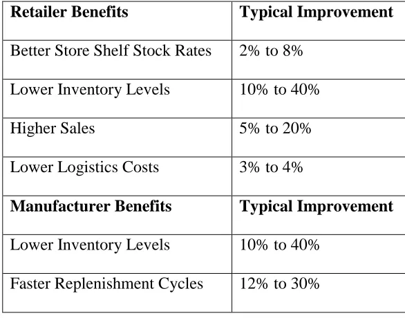
Table 2.5 Typical CPFR benefits (Sheffi, 2002) ... 20

Table 3.1 Global Compound Index Calculation ... 39

Table 5.1 Classification Assessment... 55

(10)

LIST OF FIGURES

Figure 2.1 AHP criteria priorities for supplier selection in the semiconductor assembly

equipment manufacturing industry (Chan & Chan, 2004) ... 5

Figure 2.2 Frequency of supplier selection criteria in scientific articles (Inemek & Tuna, 2009) ... 6

Figure 2.3Activities in the CPFR process (Danese, 2007) ... 19

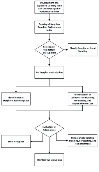
Figure 2.4: Research Framework ... 27

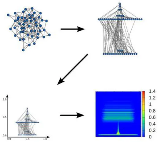
Figure 3.1 Diagram illustrating the process of visualizing an ensemble of networks. (Mones et al., 2012) ... 33

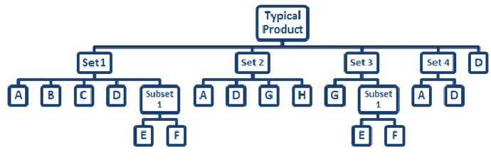
Figure 3.2 Typical Product ... 34

Figure 3.3 Path to find part criticality ... 35

Figure 3.4 Random Short Run Pareto Chart ... 40

Figure 3.5 Long Run Pareto Chart ... 41

Figure 3.6 Boeing 787 Breakdown ... 42

Figure 3.7 Countries Supplying Parts for Boeing Charleston... 42

Figure 3.8 Potential Aerospace Suppliers in South Carolina ... 43

Figure 4.1 Steps taken in this chapter ... 45

Figure 5.1 Switching Cost Breakdown ... 56

Figure 6.1 CPFR Model – Collaboration Tasks (VICS, 2004) ... 64

Figure 6.2 CPFR Steps ... 65

Figure 6.3 CPFR - Step 1 ... 66

(11)

Figure 6.7 CPFR - Steps 5 and 6... 70

Figure 6.8 CPFR - Step 7a ... 71

Figure 6.9 CPFR - Step 7b ... 72

Figure 7.1 AHP Hierarchy Diagram ... 77

Figure 8.1 The interface's main tab ... 79

Figure 8.2 Welcome tab ... 79

Figure 8.3 Parameters tab ... 80

(12)

CHAPTER 1 INTRODUCTION

1.1PREAMBLE

Supplier’s performance is an important determinant of a firm’s competitive

advantage. According to Krause et al. (2001), cost, quality, and delivery measures are often

used to conceptualize purchasing performance. Supplier’s performance evaluation on

operational criteria significantly influences cost, quality, delivery, and flexibility

dimensions of purchasing performance in US-based manufacturing companies. This

suggests that selecting suppliers on operational criteria such as cost, quality, delivery, and

flexibility, as well as monitoring performance on those criteria significantly affects the

desired capability of the same criteria internally (Nair et al. 2015).

The final product will not meet customer standards if poor-quality parts and

materials are used (Bowersox et al. 2002). The quality of parts flowing through a

manufacturing supply chain toward the original equipment manufacturer (OEM) can be

viewed in several ways:

• Quality of each part overall (conforming or non-conforming)

• Quality of each part in some key quality characteristic, Y

• Quality level of a ‘batch’ in discrete terms—percent conforming

• Quality level of a ‘batch’ in continuous terms—a distribution of quality, or

(13)

The ideal risk avoidance strategy is taking care of risks when initially selecting the

suppliers. Viswanadham and Samvedi (2013) presented the ecosystem model: it consists

of the elements within the supply chain, the entities that influence goods, information, and

financial flows through the supply chain. They demonstrate that performance is affected

by the human, financial, infrastructural and natural resources, government actions and

delivery logistics. Viswanadham and Samvedi (2013) further studied the risk contributions

of all ecosystem elements and proceed to select suppliers to minimize the risk and enhance

the performance.

Supplier evaluation is a multifaceted activity requiring the consideration of many

important characteristics. In the case of joint evaluation of co-suppliers, whom supply the

same component, previously published studies neglect stochastic co-supplier delivery

timing interactions, which can affect joint co-supplier evaluations. This study presents a

set of models that show this effect, explicitly considering the related interactions on joint

co-supplier evaluation. The computational experiments highlight the importance of the

interaction between co-suppliers and the ordering policy in supplier evaluation. It shows

the ranking of co-supplier combinations that can change significantly depending on the

ordering policy. This realization emphasizes the need to model supplier interactions and

ordering policies more accurately in the practice of supplier evaluation and selection

(Smith et al., 2006).

1.2RESEARCH OBJECTIVE AND OUTLINE

The objective of this study is to develop a framework based on a current literature

review and to lay the ground work for the development of a “Supplier’s Delivery Time and

(14)

4, and will be further developed in future work for the purpose of supplier evaluation. After

assessing supplier’s performance, a set of potential decisions regarding underperforming

suppliers is to be studied.

Section 2 is an extensive literature review covering all topics studied in this study:

(i) supplier evaluation criteria, (ii) supplier switching cost, (iii) collaborative planning,

forecasting, and replenishment (CPFR), and (iv) a subsection discussing the literature

review. Section 3 is the seedling of this project, where a part criticality index was first

developed. Following, in section 4 a detailed framework is developed based on the

literature to describe the methodology established for upcoming work starting with the

development of the Performance Index and concluding with the assessment of alternatives

regarding underperforming suppliers. Sections 5, 6, and 7 describe the alternatives an

underperforming supplier has. Section 8 shows the user interface that was developed.

(15)

CHAPTER 2 LITERATURE REVIEW

According to the Boeing suppliers’ website (Boeing Quality Management System,

2016), Boeing expects its suppliers to commit to excellent performance in terms of cost,

quality and delivery. More specifically, Boeing considers capability, capacity, reliability,

financial status, geographical location, performance, integrity, quality of product, delivery

and overall customer-supplier relations when evaluating a potential supplier before and

during the development of a purchase contract. The abovementioned reference to the

Boeing suppliers’ website was considered since this research is mainly focused on

aerospace industries and more specifically Boeing South Carolina.

In the following literature review, three main topics are discussed: (1) suppliers

evaluation criteria, (2) supplier switching cost, and (3) collaborative planning, forecasting,

and replenishment (CPFR). These topics cover the process of supplier evaluation and what

possible actions can be taken regarding underperforming suppliers. Additionally, current

research approaches dealing with supplier’s raking and the costs involved are also

(16)

2.1SUPPLIERS EVALUATION CRITERIA

According to Ho et al. (2010), 88% of the scientific articles related to suppliers’

evaluation criteria consider quality during the process of supplier selection. Additionally,

82% of those articles regard delivery as a primary criterion in supplier selection. Due to

quality and delivery maintaining the greatest significance in supplier selection, it can be

stated that the cost of products supplied is not the main criterion used by customers when

identifying their suppliers. Chan and Chan (2004) define the most important criteria for

supplier selection in the semiconductor assembly equipment manufacturing industry as

follows: quality, delivery, and cost. These were identified using the Analytical Hierarchy

Process (AHP), which is shown in Figure 2.1.

Supplier

Flexibility 0.087

Quality 0.403

Service 0.099 Cost

0.167

Innovation 0.058 Delivery

0.186

Figure 2.1 AHP criteria priorities for supplier selection in the semiconductor assembly equipment manufacturing industry (Chan & Chan, 2004)

In addition, Abdolshah (2013) ranked suppliers based on a literature review of 21

articles, where quality was ranked first among supplier evaluation criteria, followed by

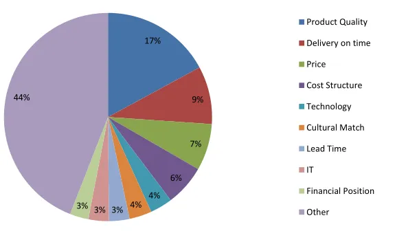
delivery and performance history. Founded on the frequency of appearance in previous

studies, the primary criteria utilized in the supplier selection process is summarized in the

(17)

Figure 2.2 Frequency of supplier selection criteria in scientific articles (Inemek & Tuna, 2009)

Based on the literature, and according to Şen et al. (2008), the main criteria used

when selecting suppliers are product quality, delivery, and service. The tables shown below

identify the different attributes mentioned in previous scientific articles. These attributes

are divided into 4 main categories: product quality, service quality, process quality, and

delivery. With respect to prime literary resources, (i) product quality and (ii) product

delivery are clearly the most prevalent attributes when evaluating a supplier (Chan & Chan,

2004; Inemek & Tuna, 2009). The upcoming subsections will dive into these two criteria

in order to understand them more and see how literature is trying to quantify them.

2.1.1Product Quality Criteria

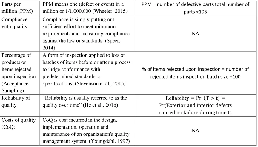
The primary attributes of product quality discussed by Ho et al. (2010) are listed

below in Table 2.1 Supplier evaluation criteria based on product quality. These attributes

are directly related to the proportion of defects and quality of incoming deliveries.

Table 2.1 Supplier evaluation criteria based on product quality

Attributes Definition Metrics

17%

9%

7%

6%

4% 4% 3% 3% 3% 44%

Product Quality

Delivery on time

Price

Cost Structure

Technology

Cultural Match

Lead Time

IT

Financial Position

(18)

Parts per million (PPM)

PPM means one (defect or event) in a million or 1/1,000,000 (Wheeler, 2015)

PPM = number of defective parts total number of parts ∗106

Compliance with quality

Compliance is simply putting out sufficient effort to meet minimum requirements and measuring compliance against the law or standards. (Speer, 2014) NA Percentage of products or items rejected upon inspection (Acceptance Sampling)

A form of inspection applied to lots or batches of items before or after a process to judge conformance with

predetermined standards or

specifications. (Stevenson et al., 2015)

% of items rejected upon inspection = number of rejected items inspection batch size ∗100

Reliability of quality

“Reliability is usually referred to as the quality over time” (He et al., 2016)

Reliability = Pr (T > t) = Pr (Exterior and interior defects caused no failure during time t)

Costs of quality (CoQ)

CoQ is cost incurred in the design, implementation, operation and

maintenance of an organization's quality management system. (Youngdahl, 1997)

NA

2.1.2Product Delivery Criteria

Attributes that fall under this criterion include appropriateness of the delivery date,

compliance with due date, delivery mistakes, number of shipments to arrive on time, and

percentage of orders shipped to buyer on or before original promised ship date (Ho et al.,

2010).

Table 2.2 Supplier evaluation criteria based on delivery

Attributes References

Appropriateness of the delivery date Ho et al., 2010; Hashemi et al., 2015 ; Simić et al., 2014 ; Onder & Kabadayi, 2015

Compliance with due date Ho et al., 2010; Hashemi et al., 2015 ; Amindoust & Saghafinia, 2013 ;

Delivery mistakes Ho et al., 2010

Number of shipments to arrive on time

Ho et al., 2010; Hashemi et al., 2015 ; Azadi et al., 2015

Percentage of orders shipped to buyer on or before original promised ship date

Ho et al., 2010

Concluding that the evaluation of suppliers is primarily derived from the product’s

(19)

index founded upon these two attributes represent the performance of a supplier. This

performance index is presented as the “Supplier’s Delivery Time and Delivered Quality

Performance Index.”

2.2SUPPLIER SWITCHING COST

In regards to an underperforming supplier, action to improve the status quo

(increase productivity) is essential. For such an unfortunate circumstance, companies are

confronted with deciding whether or not to take action; either by terminating the

relationship and looking elsewhere for the product, or by increasing collaboration with the

supplier. Both possibilities must be evaluated carefully due to related costs. The first option

results in what is known as supplier switching costs, i.e. monetary or nonmonetary costs

accumulated when switching from one supplier to another (Colwell et al., 2011).

Burnham et al. (2003) defines switching costs as the onetime costs that customers

associate with the process of switching from one provider to another. Different facets of

switching costs that a customer might encounter are: economic risk costs, evaluation costs,

learning costs, setup costs, benefit loss costs, monetary loss costs, personal relationship

loss costs, and brand relationship loss costs. Further study has then categorized these facets

into three main types: procedural switching costs, financial switching costs, and relational

switching costs (Vigolo & Cassia, 2014; Burnham et al., 2003; Vasudevan et al., 2006).

Definitions of these types and facets are provided below:

2.2.1Procedural Switching Costs

Procedural Switching Costs primarily involve the expenditure of time and effort.

• Economic Risk Costs: Uncertainty when obtaining a new supplier, due to

(20)

conceptualizing consumption risk, three of which are relevant: performance

risk, financial risk, and convenience risk (Bettman, 1973).

• Evaluation Costs: Before making the decision to switch, time and effort is

devoted to searching and analysing potential providers. Collecting

information about the suppliers is needed, as well as mental effort to analyse

such information, in order to make an informed decision.

• Learning Costs: When switching to a new provider, there are skills and

knowledge that must be acquired to effectively use the new product. Time

and effort in relation to developing these new skills and knowledge are

necessities when adapting to a new supplier.

• Setup Costs: Initiating a new relationship and/or developing the essentials

to use a new product require time and effort. In relation to services, an

abundance of information is exchanged between the new provider and the

customer concerning selling risks and the customers’ specific needs.

2.2.2Financial Switching Costs

Financial Switching Costs involve the loss of financially quantifiable resources.

• Benefit Loss Costs: Terminating a contract with a firm is likely to imply

that the economic benefits that were once accumulated are now null and

void. Discounts or benefits once acquired from the original supplier are now

lost, due to the fact that they do not transfer.

• Monetary Loss Costs: Payments that are a one-time commitment when

initially switching suppliers, not including the purchase of the new product.

(21)

monetary losses could be due to the consumer having to replace co-assets

and sub-assets in relation with the new product.

2.2.3Relational Switching Cost

Relational Switching Costs involve psychological or emotional discomfort due to

the loss of identity and the breaking of bonds.

• Personal Relationship Loss Costs: Bonds of identification are formed with

the supplier’s employees, thus, upon switching, those bonds break. The

consumer developed a level of comfort with these employees, and that is

not readily available with the new provider.

• Brand Relationship Loss Costs: Bonds of identification are formed with

incumbent suppliers, thus, upon switching, those bonds break. Brand- or

company- based relational bonds are formed due to customers drawing

meaning from their associations, which became a part of their identity.

The supplier switching cost consists of numerous expenses developed during the

process of terminating a supplier and hiring a new one. Although, it is important to

remember that not every facet is applicable for each supplier-switching situation, Zhang et

al. (2015) stated that the total switching cost is very much reliant on the quantity switched.

While they have adequately supported this claim, their classifications of the switching costs

are minimal. Zhang et al. (2015) identified setup costs, learning costs, variational costs, as

well as the compensation for the incumbent supplier, as the main concerns relating to

switching cost. Noting that the compensation for the incumbent supplier can be categorized

under “monetary costs” (Burnham et al., 2003), the payment for the incumbent supplier

(22)

soon as a contract is signed. Cancelling such a contract and switching suppliers can be

costly due to cancellation fees. These are onetime fees, which increase with the product

quantity and must be paid to the incumbent before any switch can be made. In some cases,

companies only desire to shift some of their demand to another provider. When that occurs,

the incumbent supplier adjusts the contract due to a loss of “Economies of Scale”, i.e. they

require the firm to pay a higher per unit price for the remaining products. Based on these

considerations it is reasonable to claim that switching costs are volume-dependent. Zhang

et al. (2015) also identified variational costs as an additional switching cost factor.

Variational costs develop due to the location difference of the entrant supplier; the costs

include the variation of transportation cost, communication cost, etc. (Hu et al., 2012).

Jones et al. (2002) states that when switching a provider the switching cost is

comprised of six primary cost dimensions:

• Lost performance: costs derived from the termination of a relationship

where benefits and perquisites were previously formed

• Uncertainty: costs formed due to the perceptions of risk surrounding the

performance of an unknown or untested supplier

• Pre-switching search and evaluations: costs resulting from the time and

effort involved in searching for available alternatives and evaluating their

viability prior to switching

• Post-switching behavioural and cognitive: costs formed due to the time and

effort needed to acquire and adapt to new procedures and routines

• Setup: costs derived from the perceived time and effort to relay needs and

(23)

• Sunk: costs due to the non-recoupable time, money, and effort invested in

establishing and maintaining a relationship

These dimensions resemble the facets previously defined by Burnham et al. (2003)

and Zhang et al. (2015). Due to the resemblance, these cost factors can be combined and

categorized. The resulting switching cost classifications are procedural, search &

evaluation, learning, setup, economic risk, financial, benefit loss, monetary loss, relational

(psychological), personal relationship loss, brand relationship loss, and variational. Table

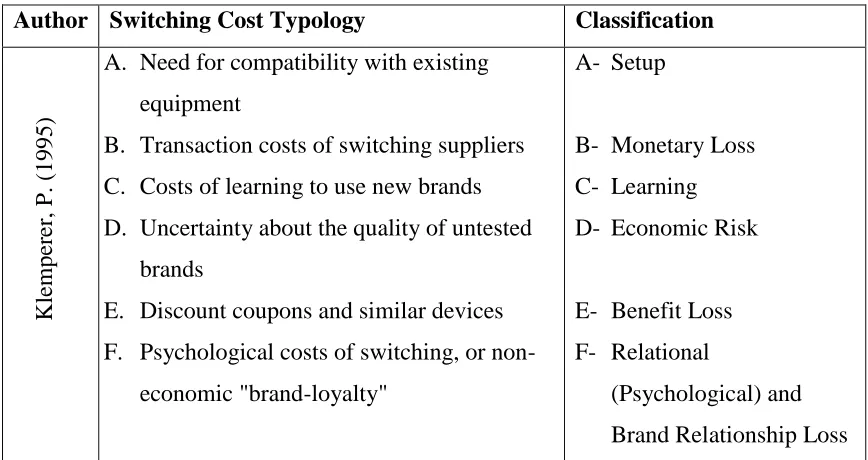
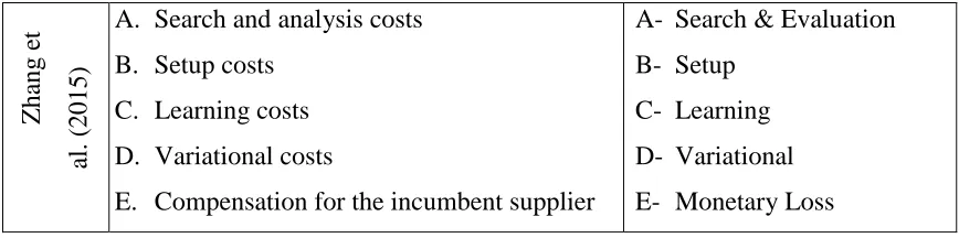
2.3 catalogues these classifications from prior switching cost typologies developed in

literature.

Table 2.3 Review of switching cost typology in literature

Author Switching Cost Typology Classification

Kle

mper

er, P. (1995)

A. Need for compatibility with existing

equipment

B. Transaction costs of switching suppliers

C. Costs of learning to use new brands

D. Uncertainty about the quality of untested

brands

E. Discount coupons and similar devices

F. Psychological costs of switching, or

non-economic "brand-loyalty"

A- Setup

B- Monetary Loss

C- Learning

D- Economic Risk

E- Benefit Loss

F- Relational

(Psychological) and

(24)

Jone

s e

t al. (

2002)

A. Continuity costs:

a. Lost performance costs

b. Uncertainty costs

B. Learning costs:

a. Pre-switching search and evaluation

costs

b. Post-switching behavioural and

cognitive costs

c. Setup costs

C. Sunk costs

A- Benefit Loss

a- Benefit Loss

b- Economic

Risk

B- Learning

a- Search & Evaluation

b- Personal Relationship

Loss and Variational

c- Setup

C- Relational

(Psychological)

B

urnha

m et a

l. (2003)

A. Procedural switching costs:

a. Economic risk costs

b. Evaluation costs

c. Learning costs

d. Setup costs

B. Financial switching costs:

a. Benefit loss costs

b. Monetary loss costs

C. Relational switching costs, or

psychological cost:

a. Personal relationship loss costs

b. Brand relationship loss costs

A- Procedural

a- Economic

Risk

b- Search &

Evaluation

c- Learning

d- Setup

B- Financial

a- Benefit Loss

b- Monetary

Loss

C- Relational

(Psychological)

a- Personal Relationship

Loss

b- Brand Relationship

(25)

Va

sude

va

n

et al. (

2006)

A. Procedural switching costs

B. Financial switching costs

C. Relational switching costs:

D. Setup costs

E. Termination costs, including the

relationship specific investments that have

no value outside the relationship

A- Procedural

B- Financial

C- Relational

(Psychological)

Loss

D- Setup

E- Benefit Loss and

Monetary Loss

W

hit

ten & W

ake

fi

eld (2

006)

A. Uncertainty costs

B. Post-switching behavioural and cognitive

costs

C. Setup costs

D. Hiring and retraining costs

E. System upgrade costs

F. Lost benefit costs

G. Pre-switching search and evaluation costs

H. Sunk costs

A- Economic Risk

B- Personal Relationship

Loss and Variational

C- Setup

D- Setup and Learning

E- Monetary Loss

F- Benefit Loss

G- Search & Evaluation

H- Relational (Psychological) C olwe ll e t al. (2011 )

A. Time costs

B. Effort costs

C. Efficiency costs

D. Training costs

E. Knowledge costs

F. Social connection costs

A- Procedural

B- Procedural

C- Setup and Variational

D- Learning

E- Learning

F- Relational

(26)

P

hua

, Y.S. (2011)

A. Supplier search costs to identify and select

suppliers

B. Contracting costs to negotiate and write

contracts

C. Transition costs to oversee the transfer of

operations and assess supplier processes

prior to contract execution

D. Monitoring and enforcement costs to

ascertain compliance with contractual

obligations and to sanction noncompliant

behaviour

E. Adjustment costs to correct for any

subsequent misalignment

F. Costs to build and maintain trust

A- Search & Evaluation

B- Monetary Loss

C- Monetary Loss and

Variational

D- Setup and Learning

E- Setup and Economic

Risk F- Relational (Psychological) B arr oso & P icón (2012 )

A. Benefit loss costs

B. Personal relationship loss costs

C. Economic risk costs

D. Search and evaluation costs

E. Setup costs

F. Monetary loss costs

A- Benefit Loss

B- Personal Relationship

Loss

C- Economic Risk

D- Search & Evaluation

E- Setup

(27)

Hu e

t al. (

2012)

A. Searching costs

B. Setup costs

C. Learning costs

D. Variational costs

E. Compensation for the incumbent supplier

F. Procedural costs

G. Financial costs

H. Relationship loss costs

I. Information sharing loss costs

B- Setup

C- Learning

D- Variational

E- Monetary Loss

F- Procedural

G- Financial

H- Relational

(Psychological)

I- Personal Relationship

Loss

Vigol

o & C

assi

a (201

4)

A. Procedural switching costs:

a. Economic risk costs

b. Evaluation costs

c. Learning costs

d. Setup costs

B. Financial switching costs:

a. Benefit loss costs

b. Monetary loss costs

C. Relational switching costs:

A- Procedural

a- Economic Risk

b- Search & Evaluation

c- Learning

d- Setup

B- Financial

a- Benefit Loss

b- Monetary Loss

C- Relational

(Psychological)

Loss

Hu e

t al. (

2014)

A. Investigation, analysis, and evaluation

costs

B. Setup costs

C. Learning costs

D. Variation of transportation costs

B- Setup

C- Learning

D- Variational

(28)

Zha

ng e

t

al. (2015)

A. Search and analysis costs

B. Setup costs

C. Learning costs

D. Variational costs

B- Setup

C- Learning

D- Variational

E- Monetary Loss

The applied literature established multiple switching cost typologies, from which

we drew our cost factor classifications. Table 2.3 catalogues the associated cost factors

from these investigated typologies. The literature review in Table 2.4 is constructed as a

tabulated structure of the classifications made per research article in Table 2.3. The

intention of Table 2.4 is to provide an easy assessment to justify the chosen switching cost

classifications.

Table 2.4 Classification assessment

P ro ce du ra l Sear ch & E v alu atio n L ea rn in g Setu p E co n o m ic R is k F ina ncia l B en ef it L o ss Mo n etar y L o ss Rela tio na l ( P sy cho lo g ica l) Per so n al R elatio n sh ip L o ss B ran d R elatio n sh ip L o ss Va ria tio na l

Klemperer, P. (1995) * * * * * * *

Jones et al. (2002) * * * * * * * *

Burnham et al. (2003) * * * * * * * * * * *

Vasudevan et al. (2006) * * * * * * * *

Whitten & Wakefield (2006) * * * * * * * * *

Colwell et al. (2011) * * * * *

Phua, Y.S. (2011) * * * * * * *

Barroso & Picón (2012) * * * * * *

(29)

Vigolo & Cassia (2014) * * * * * * * * * * *

Hu et al. (2014) * * * * *

Zhang et al. (2015) * * * * *

Total 5 9 10 12 7 4 7 10 9 7 4 7

Based on the acknowledged cost factors within each literary article in Table 4, it is

evident that our switching cost classifications are supported throughout literature. The

primary factors identified as procedural, financial, and relational (psychological) are

derived from research conducted by Burnham et al. (2003). These switching cost types

encompass the majority from which supplier switching costs originate. This is supported

due to the fact that other researchers identified them within their switching cost typologies.

In the case they were not identified, the researchers’ cost factors included their sub-facets.

Procedural cost sub-facets are search & evaluation, learning, setup and economic risk;

financial cost sub-facets are benefit loss and monetary loss; and relational (psychological)

cost sub-facets are personal relationship loss and brand relationship loss. Lastly, our final

classified switching cost factor, variational, is also supported throughout literature. This is

evident by the 7 out of 12 typologies that include such variational costs. As a result, Table

4 justifies the initial cost factors constructed by Burnham et al. in 2003, as well as

variational costs identified by Zhang et al. in 2015 as implicated costs when switching a

supplier.

2.3COLLABORATIVE PLANNING, FORECASTING, AND REPLENISHMENT

(CPFR)

When a supplier is underperforming, it becomes important for the customer to

create a plan of action regarding the supplier. In order to do this, the customer is faced with

(30)

supplier. Each of these tasks comes with a cost and the one with the lower cost should be

chosen. In this study, we will create a model that will help determine the cost to a retailer

of implementing Collaborative Planning, Forecasting, and Replenishment (CPFR). To do

this we will calculate the time it takes to make the equivalent improvements of switching

suppliers through the improvement of CPFR. The time will be calculated using a system

dynamics and supply chain research.

2.3.1CPFR Background

Definition. Collaborative Planning, Forecasting, and Replenishment (CPFR) is one

of the newest and highly acknowledged approaches to inventory management, and

provides a holistic method to improving supply chain integration (Varma & Bansal, 2010).

It was created in 1998 by Voluntary Interindustry Commerce Solutions (VICS) committee

and has the goal of increasing collaboration through improved planning, forecasting, and

replenishment processes by increasing data and forecast sharing based on customer demand

(Voluntary Interindustry Commerce Solutions, 2007). The basic process to achieve these

results was laid in steps in that can be summarized by (1) creating a front-end agreement,

(2) generating a joint business plan, (3) development of demand forecasts, (4) sharing

forecasts, and (5) inventory replenishment (Fliedner, 2003).

Develop Front End Agreement Create Joint Business plan Create Sales Forecast Identify Exceptions To Sales Forecast Resolve Exceptions To Sales Forecast Create Order Forecast Identify Exceptions To Order Forecast Resolve Exceptions to Order Forecast Generate Order

PLANNING FORECASTING REPLENISHMENT

Figure 2.3 Activities in the CPFR process (Danese, 2007)

Benefits. The basic premise of CPFR is that by allowing the supply chain to

(31)

The benefits help both the supplier and vendor’s companies increase productivity as

positive business practices are at the base of CPFR (Voluntary Interindustry Commerce

Solutions, 2007). Some of the most common benefits:

 Retailer benefits: increased sales and higher service levels

 Manufacturer benefits: higher order fill rates and faster cycle times

 Shared benefits: improved forecast accuracy and lower system expenses (Fliedner,

2003)

In addition, CPFR consistently shows a larger increase in supply chain performance

than other standard practices (Danese, 2007). When Ryu (2006) conducted a study between

consignment, VMI 1, VMI 2 and CPFR, CPFR was found to improve supply chain profit

most significantly. Disney et al. (2004) demonstrated using a Beer game simulation that

CPFR helped to reduce the bullwhip more significantly then VMI (Ryu, 2006; Fliender,

2003; Disney et al., 2004). Campo et al. (2003) pointed out that inadequate inventory would

reduce the amount of future purchase from the customers.

Table 2.5 Typical CPFR benefits (Sheffi, 2002)

Retailer Benefits Typical Improvement

Better Store Shelf Stock Rates 2% to 8%

Lower Inventory Levels 10% to 40%

Higher Sales 5% to 20%

Lower Logistics Costs 3% to 4%

Manufacturer Benefits Typical Improvement

Lower Inventory Levels 10% to 40%

(32)

Higher Sales 2% to 10%

Better Customer Service 5% to 10%

Implementation. There are many different levels, types, and intensities of

implementation. Depending on the partners involved, the roles in creating forecasts and

orders will be affected (Voluntary Interindustry Commerce Solutions, 2007). Many

companies begin with a pilot program, and depending on the success decide to expand

CPFR to other products and suppliers (Panahifar et al., 2015). Companies and researchers

are also continuously improving the base framework provided for CPFR. Several

improvements that have been made are IT software, modelling techniques, and

identification of key inhibitors and enablers.

Inhibitors. Though the rewards of CPFR can be great, implementation is not an

easy task (Barratt & Oliveira, 2001; Danese, 2007). Despite CPFR’s initial excitement,

relatively few companies have implemented CPFR in their supply chains (Barratt &

Oliveira., 2001). This is largely due to inhibiting factors and barriers, which can be divided

into four categories: managerial, process, technological, and cultural (Panahifar et al.,

2014). In addition, the barriers can take the form of either intra-company or inter-company

issues (Panahifar et al., 2015). The largest inhibiting factors found by Panahifar et al.

(2014) using ISM analysis are lack of leadership, lack of technical expertise, difficulties in

information sharing and lack of compatibility of partner’s abilities. Barret et al. (2001)

found through a survey that trust, scalability, and lack of software were some of the key

barriers. Lastly, Terwiesch et al. (2005) used an empirical analysis to conclude that even

(33)

Enablers. Unlike inhibitors, enabling factors help with the implementation of

CPFR in supply chains. There has been considerable research and case studies to identify

the factors that allow for the practical applications of CPFR (Voluntary Interindustry

Commerce Solutions, 2007; Barratt & Oliveira, 2001; Panahifar et al., 2015; Fu et al.,

2010; Panahifar et al., 2015(2)). These enablers are interconnected and as they improve,

other enablers will improve, as will the supply chain as a whole. Panahifar et al. (2015)

uses a survey sent to many of the leading experts in CPFR implementation to find, rank,

and tier the main enablers. It is found that competition pressure is the most significant

enabler and drives factors such as, senior management support and clear communication

planning. In another study, Fu et al. (2010) implemented fuzzy AHP analysis and a

questionnaire to determine the key enablers regarding technology, organization, and

environment.

2.3.2Models/Simulations of CPFR

There have been numerous attempts at modelling the effects of CPFR on a supply

chain system to compare different collaboration models and calculate the potential benefits

of CPFR. Several models investigate the effects of increased collaboration on reducing

bullwhip effects (Disney et al., 2004; Ryu, 2006). Others compare different collaboration

techniques and provide monetary cost reductions according to different variables in

simulations (Disney et al., 2004; Sari, 2008; Ryu, 2006). These simulations are important

(1) to validate our choice in using CPFR to increasing collaboration and evaluating a cost

function and (2) to understand the different modelling techniques and variables used in

(34)

Aviv (2001, 2002, and 2007) has made significant contributions to the modelling

of CPFR. In 2001, Aviv looks at a cooperative, two stage supply system consisting of a

retailer and supplier. The comparison is made between a supply chain where inventory and

forecast information is only known locally vs. a single forecast system being jointly

maintained. Aviv uses lead times, holding costs, backorder demand to calculate the total

costs to the partners. Aviv found that the absolute benefits of CPFR are a cost reduction of

19.43% and the marginal benefits are 9.56% (Aviv, 2001). Aviv continued with this work

in 2002 by presenting a similar simulation using a demand that evolves an auto-regressive

time series. The research brings a sharper focus showing that Vendor Managed Inventory

(VMI) and Collaborative Forecasting (CF) programs become more important as the

demand process is correlated across periods (Aviv, 2002). According to Torkul et al.

(2016), many factors can increase the inventory holding costs: (1) variation of demand, (2)

large safety stock. Aviv investigates CF partnerships where the supply chains are capacity

constrained. The model addresses three specific components: (1) co-evolution of demand

and information, (2) supply chain scorecard, and (3) production and inventory policies. The

model demonstrates how the benefits of CF can be unevenly split (Aviv, 2001). Finally, in

2007 Aviv creates another simulation that investigates the optimal relative explanatory

power of the partners (Aviv, 2007).

Disney et al. (2004) investigates how the different collaboration models can work

together with the growth of e-commerce. The Beer Game he developed is used to calculate

the impact of the bullwhip effect using five supply chains types created from a combination

internet, communications technologies (ICT), and collaboration methods. The model uses

(35)

effect and the e-shopping supply chain, where all information is immediately shared with

all parties, has the greatest reduction in the bullwhip effect.

Sari (2008) explores the appropriate level of collaboration between partners

depending on business conditions. A simple model is created using a traditional supply

system and two that involve VMI and CPFR. The findings demonstrate that the benefits

are always greater using CPFR, but sometimes the additional resources do not justify the

improvements.

Ryu (2006) compared five different supply chains methods (traditional,

consignment, VMI1, VMI2, and CPFR) to find the largest reduction in total costs. At first

an analytical approach is used to determine profit maximization. CPFR showed the largest

supply chain profit, though the benefits were skewed towards the supplier. Then, a supply

chain system model was implemented to look at how six different independent variables,

one of which was coordination mechanism, affected the dependent variables: economic

measure, customer satisfaction, and the bullwhip effect. In all, it was found that CPFR

produces the most supply chain profit, but collaboration mechanisms that focused wholly

on profit maximization may lead to a decrease in performance regarding variables such as

customer service and the bullwhip effect.

2.4LITERATURE REVIEW SUMMARY AND DISCUSSION

Based on the literature regarding suppliers’ evaluation criteria, it was established

that product quality and product delivery are the primary criteria used to evaluate suppliers

on their performance. In this study, the proportion of defective supplied parts by supplier

and lateness of deliveries will be used in the development of the suppliers’ Delivery Time

(36)

The facets developed by Burnham et al. (2003) are the basis on which our supplier

switching cost research is derived. It is evident from the literature review in Table 4 that

the three main switching cost types (procedural, financial, and relational) encompass the

majority from which supplier switching costs originate. Some authors identify the main

types as a cost factor, while others identify the specific facets that form these types.

Furthermore, the literature identified variational as an additional cost factor. Variational

costs were unable to be classified within any previously defined switching cost factor, thus

the decision to include it as its own dimension. The resulting cost factors from which the

supplier switching cost is developed are procedural, financial, relational, and variational

costs. It is important to state that in every supplier-switching situation, not every type

and/or facet is appropriate to account for, but with that said, the majority of these costs will

arise in any supplier switching transition.

CPFR is realized to be an effective method to enhance not only collaboration with

suppliers but also suppliers’ performance.

2.4.1Research Framework

After understanding the current practices utilized for supplier assessment and the

valuation of possible actions taken regarding underperforming suppliers, the below

research framework (Figure 2.4) was developed. This framework will be applied in future

work, where focus will be on the development of models for supplier evaluation and

decision-making.

The framework first identifies the development of the Supplier’s Delivery Time

and Delivered Quality Performance Cost Function. Established from this cost function,

(37)

placed under review and the suppliers’ switching cost and the cost of collaborative

planning, forecasting and replenishment (CPFR) will be developed, so that an easy

comparison can be made between these two alternatives and the current cost.. The next

step will be to decide whether to switch suppliers, increase collaboration, or maintain the

status quo. In order to make such a decision an analytical hierarchy process (AHP) will be

developed to choose between the alternatives based on cost, feasibility, and management

willingness.

Based on the literature review, it became evident that the main attributes

implemented when assessing suppliers are the delivery time and delivered quality. Hence,

the introduction of an index founded upon these two attributes; recognized as the

“Supplier’s Delivery Time and Delivery Quality Performance Index.” This index

represents the performance of suppliers and is necessary for further development into

supplier evaluation. When faced with an underperforming supplier, management evaluates

whether to switch their demand to a new supplier or to increase collaboration with the

incumbent supplier, so that the current performance may be enhanced. This decision is

primarily prompted by the cost of each alternative.

Cost models for these alternatives are necessary for management to come to an

informed decision, one to calculate the potential cost of switching suppliers and the other

to calculate the potential cost of collaborative planning. These two models adjacent to the

current cost would aid in the assessment of the alternatives: (1) maintain the status quo, (2)

(38)

Development of a Supplier’s Delivery Time

and Delivered Quality Performance Index

Ranking of Suppliers Based on Performance

Index

Identification of Collaborative Planning,

Forecasting, and Replenishment Cost

Switch Supplier

Increase Collaborative Planning, Forecasting, and

Replenishment Selection of

the Bottom 5% Suppliers

Classify Supplier as Good Standing

Put Supplier on Probation

Identification of Supplier’s Switching Cost

Evaluation of Alternatives

Maintain the Status Quo

(39)

The current evaluation process norm is to study the alternatives and then make an

“educated guess,” a decision primarily based on intuition. A more reliable evaluation

system is possible by further assessment using an analytical evaluation using these cost

models accompanied by the Analytical Hierarchy Process (AHP). The Analytical

Hierarchy Process (AHP) is a theory developed in 1977 by Thomas L. Saaty based on

pairwise comparison and connoisseurs’ judgments to generate the priority scale (Saaty,

2008). AHP is a multi-criteria decision making tool providing an approach to identify

interaction among multiple decision factors (Barker & Zabinsky, 2011). In future work, the

AHP will be an integral part in the assessment of supplier alternatives, along with a

(40)

CHAPTER 3 DEVELOPMENT OF A PART CRITICALITY INDEX IN INVENTORY

MANAGEMENT

As businesses grow in size, inventory management analysis is becoming more

important to increase efficiency and profits by reducing backorders and surpluses. Part of

this change is a result of limited in house production of parts and a focus on final assembly,

which creates a need to evaluate part criticality in the supply chain. The two fundamental

problems that arise from a poor supply chain are a large backlog and surplus. The

percentage of items backordered and the number of backorder days are important measures

of the quality of a company's customer service and the effectiveness of its inventory

management. On the other hand, if the business has an inventory surplus it will incur costs

to store, track and insure inventory. Therefore, creating an inventory management system

that ranks part criticality based on their creation of backorders and surpluses can create

significant financial and customer service improvements for a business.

Two common inventory-management strategies are the just-in-time (JIT) method,

where companies plan to receive items as they are needed rather than maintaining high

inventory levels, and materials requirement planning (MRP), which schedules material

deliveries based on sales forecasts. JIT means that manufacturers and retailers keep only

(41)

insurance costs, as well as the cost of liquidating or discarding unused, unwanted inventory.

To balance this style of inventory management, manufacturers and retailers must work

together to monitor the availability of resources on the manufacturer’s end and consumer

demand on the retailer’s. The MRP inventory management method is sales-forecast

dependent. This means that manufacturers must have accurate sales records to enable

accurate planning of inventory needs and to communicate those needs with materials

suppliers in a timely manner. These methods are geared towards supply chain management

and are concerned with when certain products are to be ordered but do not incorporate in

what order and whether they should be ordered. Overall, these methods view all parts as

having equal importance and miss the part criticality tier that helps account for

imperfections and differentiation between different parts that affect production time.

To achieve a balance between efficient customer service and low inventory cost, an

optimization model should be set in place that finds a part that is most critical amongst the

bills of material. Companies cannot spread their recourses equally amongst all the products

and inventory management. By defining the most important parts companies will be able

to more efficiently delegate their resources. In order to do this, an algorithm will be created

using different components of existing part criticality models found through a literature

review. Then the part criticality index will be generated in order to target critical parts on

the inventory floor and will be simulated through randomly generated number tests.

Finally, the system will be placed in a real world application to test its effectiveness.

As business and production facilities grow in size and complexity, inventory and

supply chain management have grown increasingly important to gain an upper edge.

(42)

(Lambert and Cooper, 2000). A large part of this supply chain is material requirement

planning and safety stock decisions. With the cost of holding inventory as high as 40% of

the inventory value, it is important to maintain the optimal amount (Sandyig and Reistad,

2000).

Modeling and determining the optimal amount of inventory depends on several

factors. Depending on the company size, either a single or a multi-echelon system should

be put in place. If the model represents a single entity, such as a warehouse, a single echelon

model is used. Multi-echelon, composed of many single-echelon systems, models are used

most often due to current companies size (Hausman and Erkip, 1994). Finally, event

occurrences can be assigned numbers, deterministic or stochastic, when creating inventory

models. All these variables create a variety of inventory management policies.

The first part criticality inventory system investigated is the spare parts theory,

which involves the assignment of criticality to the parts that make up the manufacturing

equipment. Due to the high uncertainty of the requirement of the spare parts and small

amount of suppliers, spare parts are inherently difficult to manage. This generally causes a

large amount of overstocking (Roda et al., 2014). In order to deal with these issues, spare

parts are generally put into categories in order help create proper stocking. Drekker began

this by allowing equipment criticality to determine the stock of spare parts by assigning

each piece of equipment a status of either “critical and non-critical” (Dekker et al., 1998).

In order to determine the optimal order quantity and reorder point for aircraft spare

parts, Aisyati et al. (2013) used a continuous review model. The suggested model resulted

in smaller total cost compared with existing policy. An ABC classification system was used

(43)

commonly known as important classes. The result from the research indicates that the

continuous review policy gives a significant amount of saving compared to the pre-existing

policy. Finally, in order to expand on the ABC model, Stoll et al. (2015) used a three

dimensional approach allowing for the predictability of demand and importance of the part

to be calculated in. The spare part inventory theories lay the groundwork for determining

the criticality of different parts of a production facility.

Another way to examine the importance of a part is to investigate the intricate web

of the interactions among the units of related systems. One of the most successful recent

approaches to capturing the fundamental features of the structure and dynamics of complex

systems has been the investigation of the networks associated with the units (nodes)

together with their relations (edges). Mones et al. (2012) developed an approach and

proposed a measure capable of capturing the essential features of the structure and the

degree of hierarchy in a complex network. The measure introduced is based on a

generalization of the m-reach centrality, which is first extending to directed/partially

directed graphs. Then, a global reaching centrality (GRC) was defined, which is the

difference between the maximum and the average value of the generalized reach

centralities over the network. Results for real networks show that the hierarchy measure is

(44)

Figure 3.1 Diagram illustrating the process of visualizing an ensemble of networks. (Mones et al., 2012)

Manzini et al (2015) uses the method of nodes and edges to create a system to deal

with manufacturing-to-order and assembly-to-order processes. Since each product is

unique there is no large part inventory to pick from. To formalize the utilization of the part

in the production, Manzini lets the source node be when the part is introduced and the sink

node be the milestone before the production operation requiring the component. Then to

evaluate the criticality of the part, Manzini finds the overlap of the probability that the

component is needed in the production operation and the probability that component has

not arrived. An overlap of these provides a risk that determines the criticality of the part.

The system of edges and nodes works well in production lines because of the step-by-step

nature of manufacturing facilities.

3.1DEFINING THE PART CRITICALITY INDEX

The solution employed in this study focuses on the idea on part Criticality in

(45)

• The spare parts inventory management technique where equipment spare

parts are assigned a value due to their criticalness to the production line (Dekker et al.,

1998).

• The system of nodes and edges Mones et al. put forward to describe the

fundamental features and hierarchies of a structure and dynamics of complex systems

(Mones et al., 2012).

Figure 3.2 Typical Product

Combining these two systems gave a unique approach to determining the part

criticality. The spare parts inventory management system introduced the concept of

backlogs and order demand to part criticality while the system of nodes and edges allowed

for the complex system of a product and production line to be simplified and quantified.

The system of nodes and edges can be applied to a production line if the nodes are

looked at as parts and edges being the assembly links. If a part is out of stock, this cuts off

connections not allowing the production to flow through the map to the final assembly. The

most critical parts of a product then become the parts with the most connections due to

their ability to cut off more of the production line and are therefore given preference in

stocking systems. The spare part inventory technique was used to rank the product

criticality by including the demand and backlog. This way the most important part could

(46)

will helps envision the bigger supply chain later in order tackle criticality not only on the

factory floor but by reaching suppliers and enhancing the cooperation between all the

supply chain entities. A general approach for the creation of each factor in the methodology

is listed below followed by a more detailed approach.

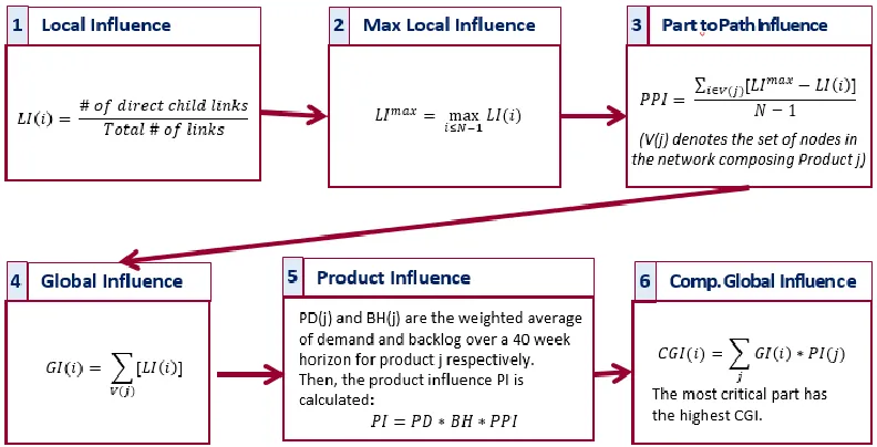
Figure 3.3 Path to find part criticality

3.1.1Local Influence

The first step is to define the local influence of a certain node i (nodes in this case

represent parts, sub-parts, and the final product) in an unweighted directed graph. The

studied network is a directed network since only parts lead to sub-parts which lead to final

product and not the other way around. The local influence, LI(i), is defined as the

proportion of all nodes in the graph that can be reached from node i via incoming edges to

i.

𝐿𝐼(𝑖) = # 𝑜𝑓 𝑑𝑖𝑟𝑒𝑐𝑡 𝑐ℎ𝑖𝑙𝑑 𝑙𝑖𝑛𝑘𝑠

𝑇𝑜𝑡𝑎𝑙 # 𝑜𝑓 𝑙𝑖𝑛𝑘𝑠 (1)

(47)

3.1.2Maximum Local Influence

After calculating local influence at all nodes, we designate LImax_{as the highest}

Local Influence. LImax will be used in the following step in order to normalize the Local

Influence to compare LI of a certain part between different products.

𝐿𝐼𝑚𝑎𝑥 = max

𝑖≤𝑁−1𝐿𝐼(𝑖) (2)

3.1.3Part to Product Influence

Thus, we can calculate the Part to Product Influence (PPI):

𝑃𝑃𝐼 = ∑ [𝐿𝐼

𝑚𝑎𝑥 _{− 𝐿𝐼(𝑖)]} 𝑖∈𝑉(𝑗)

𝑁 − 1 (3)

Note that V(j) denotes the set of nodes in the network composing Product j.

Calculating the PPI allows us compare the influence of the parts on different products.

3.1.4Global Influence

The Global Influence of a Part in a Product can be calculated as follows:

𝐺𝐼(𝑖) = ∑[𝐿𝐼(𝑖)] 𝑉(𝑗)

(4)

In other words GI(i) represents the weight of each part in a product, bigger GI(i)

shows that part i is a major component of the product.

3.1.5Product Influence and Backlog History

Calculate Product Influence and Backlog History of each product. This is an

important criterion to relate each product to the larger picture of the entire production

facility.

a. PD(j) is the weighted average of Demand over a 40 week horizon for

(48)

b. BH(j) is the weighted average backlog over a 40 week horizon for product

j.

c. Calculate the product Index PI which is the product of PPI, PD, and BH.

3.1.6Compound Global Index

The last step is to find the Compound Global Index (CGI) that represents the part

criticality among all products. The CGI brings together the most important parts and

products to find the most critical parts to the production line. To calculate CGI for each

part, we use the following equation representing the sum-product of parts Global Influence

in each product and the Product Influence:

𝐶𝐺𝐼(𝑖) = ∑ 𝐺𝐼(𝑖) ∗ 𝑃𝐼(𝑗) 𝑗

(5)

3.2INVENTORY MODEL

3.2.1Products

Six fictional products where created in order to apply the above-mentioned

algorithm. Each product consists of a set of parts, subsets, and sets. Note that subsets are

subassemblies of parts, and sets are subassemblies of parts and subsets. Creating multiple

products helps create a more realistic representation of a large final assembly production

facility.

3.2.2Supply and Demand

In this model, both supply and demand are set as constant stochastic variables. The

distribution used is the uniform distribution. Furthermore, a finite planning horizon of 40

(49)

3.2.3Inventory and Backlog

In order to perform accurate long run simulations a model was created to help us

simulate a realistic scenario where inventory is not scrapped from period to another and

unmet demand is met in the upcoming periods. In create this model inventory from one

period to another is kept and unmet demand from one period to another is backlogged.

Inventory, I(n), and shortage, S(n), for a typical period n is calculated as follows:

𝐼(𝑛) = 𝐼(𝑛 − 1) + 𝑀𝑎𝑥[ 𝑄(𝑛) − 𝐷(𝑛), 0 ]

𝐼(0) = 0

(6)

𝑆(𝑛) = 𝑆(𝑛 − 1) + 𝑀𝑎𝑥[ 𝐷(𝑛) − 𝑄(𝑛), 0 ]

𝑆(0) = 0

(7)

Note that D(n) and Q(n) represent Demand and Supply during a period n

respectively.

3.3DISCUSSION OF RESULTS

3.3.1Primitive Model

A first model was developed with the following assumptions: surplus inventory

from one term to another is scrapped and backlog is not allowed, i.e., unmet demand during

a certain period is disregarded in the next period. For this model, all random simulation led

to same result, the same part was found to be critical. But, this model is not logical since

inventory can be kept from one period to another and unmet demand is usually met in the

upcoming periods. Hence, a more realistic model was developed in order to take into

consideration surplus inventory and backlog. The integration of these parameters was

Salt Tectonism In The Carolina Trough

Scholar Commons

Development Of A Supplier’s Delivery Time And

Delivered Quality Performance Index And

Assessment Of Alternative Decisions Regarding

Underperforming Suppliers For The Aerospace

Industry

D

S

’

D

T

D

Q

P

I

A

A

D

R

U

S

F

T

A

I

ACKNOWLEDGEMENTS

ABSTRACT

PREFACE

TABLE OF CONTENTS

LIST OF TABLES

LIST OF FIGURES

CHAPTER 1

INTRODUCTION

CHAPTER 2

LITERATURE REVIEW

CHAPTER 3

DEVELOPMENT OF A PART CRITICALITY INDEX IN INVENTORY

MANAGEMENT