A novel logistic-NARX model as a classifier for dynamic binary classification

(1)

classification

.

White Rose Research Online URL for this paper:

http://eprints.whiterose.ac.uk/116081/

Version: Accepted Version

Article:

Ayala Solares, J.R., Wei, H. orcid.org/0000-0002-4704-7346 and Billings, S.A. (2017) A

novel logistic-NARX model as a classifier for dynamic binary classification. Neural

Computing & Applications. ISSN 0941-0643

https://doi.org/10.1007/s00521-017-2976-x

[email protected]

https://eprints.whiterose.ac.uk/

Reuse

Items deposited in White Rose Research Online are protected by copyright, with all rights reserved unless

indicated otherwise. They may be downloaded and/or printed for private study, or other acts as permitted by

national copyright laws. The publisher or other rights holders may allow further reproduction and re-use of

the full text version. This is indicated by the licence information on the White Rose Research Online record

for the item.

Takedown

If you consider content in White Rose Research Online to be in breach of UK law, please notify us by

(2)

(will be inserted by the editor)

A novel logistic-NARX model as a classifier for dynamic binary classification

Jose Roberto Ayala Solares · Hua-Liang Wei · Stephen A.

Billings

the date of receipt and acceptance should be inserted later

Abstract System identification and data driven modeling techniques have seen ubiquitous applications in past decades. In particular, parametric modelling methodologies such as linear and nonlinear autoregressive with ex-ogenous inputs models (ARX and NARX) and other similar and related model types have been preferably applied to handle diverse data driven modeling problems due to their easy-to-compute linear-in-the-parameters structure, which allows the resultant models to be easily interpreted. In recent years, several variations of the NARX method-ology have been proposed that improve the performance of the original algorithm. Nevertheless, in most cases, NARX models are applied to regression problems where all output variables involve continuous or discrete-time sequences sampled from a continuous process, and little attention has been paid to classification problems where the output signal is a binary sequence. Therefore, we developed a novel classification algorithm that combines the NARX methodology with logistic regression and the proposed method is referred to as logistic-NARX model. Such a combination is advantageous since the NARX methodology helps to deal with the multicollinearity prob-lem while the logistic regression produces a model that predicts categorical outcomes. Furthermore, the NARX approach allows for the inclusion of lagged terms and interactions between them in a straight forward manner resulting in interpretable models where users can identify which input variables play an important role individu-ally and/or interactively in the classification process, something that is not achievable using other classification techniques like random forests, support vector machines and k-nearest neighbors. The efficiency of the proposed method is tested with five case studies.

Keywords Nonlinear system identification·Dynamic systems·Binary classification ·NARX models·Logistic regression

1 Introduction

System identification focuses on finding models from data and use them to understand or analyze the properties or behaviours of the underlying systems [1].

Linear models have been widely used in many applications [2]. However, its applicability is limited since most of the real world problems may not be well presented using linear models [3]. Research on nonlinear system identification has been carried out and advanced since the 1980s [1]. One of the most popular methodologies is the Nonlinear AutoRegressive Moving Average with eXogenous inputs (NARMAX) methodology, which has proved to be suitable for a wide class of nonlinear systems [1,4–8]. The NARMAX approach can detect an appropriate model structure and select the most important model terms from a dictionary consisting of a great number of candidate model terms.

In recent years, several variants have been proposed that improve the performance of the original algorithm. Such variations include the use of more complex and flexible predefined functions [6,9–13], novel dependency

Jose Roberto Ayala Solares

Department of Automatic Control and Systems Engineering Faculty of Engineering

The University of Sheffield United Kingdom

E-mail: [email protected]

Hua-Liang Wei ( )

Stephen A. Billings

(3)

metrics [5,8,14–21] or different search mechanisms [22–26]. Nevertheless, the different versions of the NARX methodology have been designed under the assumption that the variables involved are continuous.

Many real-life systems involve a mixed combination of continuous and discrete variables. In this work, we focus on systems with binary responses that depend on continuous time predictors. Binary responses are commonly studied in many situations such as the presence or absence of a disease, granting a loan, or detecting the failure of a process, system or product [27,28]. However, the use of traditional regression techniques to deal with systems with a dichotomous response variable may not be appropriate given that they are sensitive to outliers and the distribution of the classes [27].

In this work, we propose a novel approach that combines logistic regression with the NARX methodology. The main motivation comes from the fact that logistic regression models are more suitable for binary classification problems given that they provide probabilities of belonging or not to a particular class. One important consid-eration when constructing a logistic regression model is multicollinearity. In general, it is important to always check for high inter-correlations among the predictor variables. In the ideal scenario, the predictor variables will have a strong relationship to the dependent variable but should not be strongly related to each other [29]. This problem is adequately solved using the NARX approach, since the model terms selected are orthogonal (uncorre-lated) to each other. Furthermore, the NARX approach allows for the inclusion of lagged terms and interactions between them in a straight forward manner resulting in interpretable models, something that is not achievable using other popular classification techniques like random forests [30], support vector machines [31] and k-nearest neighbors [32].

This work is organised as follows. Section 2 includes a brief summary of nonlinear system identification and a discussion of the Orthogonal Forward Regression algorithm. In section 3 our new methodology is described. Section 4 presents three numerical case studies that show the effectiveness of our new method. In section 5 the logistic-NARX model is applied to two real applications. Section 6 discusses advantages and disadvantages of the technique. The work is concluded in section 7.

2 Nonlinear System Identification

System identification, as a data based modelling approach, aims to find a model from available data that can represent as close as possible the system input and output relationship [1,2]. While conventionally linear models have been applied in many applications, its applicability is limited as the linearity assumption may be violated for many nonlinear system modelling problems [3]. Nonlinear system identification techniques have been ad-vanced since the 1980s [1]. In particular, the Nonlinear AutoRegressive Moving Average with eXogenous inputs (NARMAX) methodology has proved to be a powerful tool for nonlinear system identification [1,12,33,34].

In general, system identification consists of several steps, including data collection and process-ing, selection of mathematical representation, model structure selection, parameter estimation, and model validation[2].Data processing is an important part given that data preparation plays a key role when training a model. Generally, this consists of dealing with missing values and outliers, data normalization and transformation, dimensionality reduction, and performing feature engineering. In [32,35], these issues are widely discussed. Regarding the selection of mathematical represen-tation, this work focuses on NARX models. Model structure detection has been tackled using different methods like clustering [36,37], the Least Absolute Shrinkage and Selection Operator (LASSO) [38,39], elastic nets [40,41], genetic programming [42,43], the Orthogonal Forward Regression (OFR) using the Error Reduction Ratio (ERR) approach [33], and the bagging methodology [21]. Parameter estimation has been performed using the traditional least squares method, gradient descent and the Metropolis-Hastings algorithm [44,45]. Finally, for model validation, a set of statistical correlation tests have been developed in [46] and can be used to test and verify the validity of the identified nonlinear input-output models. In summary, system identification is a process that builds a parsimonious model that satisfies a set of accuracy and validity tests [10].

2.1 Orthogonal Forward Regression Algorithm

The NARX model is a nonlinear recursive difference equation with the following general form:

y(k) =f!y(k−1), . . . , y(k−ny),

u(k−1), . . . , u(k−nu)

"

+e(k) (1)

(4)

and nu [8]. Most approaches assume that the functionf(·)can be approximated by a linear combination of a

predefined set of functionsφm

!

ϕ(k)", therefore equation (1) can be expressed in a linear-in-the-parameters form

y(k) =

M

#

m=1

θmφm

!

ϕ(k)"+e(k) (2)

whereθmare the coefficients to be estimated,φm

!

ϕ(k)"are the predefined functions that depend on the regressor

vectorϕ(k) =$y(k−1), . . . , y(k−ny), u(k−1), . . . , u(k−nu)

%T

of past outputs and inputs, andM is the number of functions in the set.

The most popular algorithm for NARX modelling is the Orthogonal Forward Regression (OFR) algorithm. As a greedy algorithm [4], it adopts a recursive partitioning procedure [47] to fit a parsimonious NARX model which can be represented as a generalized dynamic linear regression problem [8,48]. One of the most commonly used NARX models is the polynomial NARX representation, where equation (2) can be explicitly written as

(3) y(k) =θ0+

n

#

i1=1

θi1xi1(k) +

n

#

i1=1

n

#

i2=i1

θi1i2xi1(k)xi2(k) +· · ·

+ n # i1=1 · · · n #

iℓ=iℓ₋1

θi1i2...iℓxi1(k)xi2(k)...xiℓ(k) +e(k)

where

(4) xm(k) =

&

y(k−m) 1≤m≤ny

u(k−m+ny) ny+ 1≤m≤n=ny+nu

andℓis the nonlinear degree of the model. A NARX model of orderℓmeans that the order of each term in the model is not higher thanℓ. The total number of potential terms in a polynomial NARX model is given by

M = '

n+ℓ ℓ

(

= (n+ℓ) !

n!·ℓ! (5)

The OFR algorithm implements a stepwise regression to select the most relevant regressors, one at a time; it uses the error reduction ratio (ERR) as an index to measure the significance of each candidate model term [1]. The OFR algorithm can be used to transform a number of selected model terms to a set of orthogonal vectors, for which ERR can be evaluated by calculating the non-centralised squared correlation coefficientC(x,y)between

two associated vectorsxandy[5]

C(x,y) =

!

xTy

"2

(xTx) (yTy) (6)

In recent years, several variants of the algorithm have been proposed that modify the predefined functions, the dependency metric or the search mechanism in order to enhance its performance. In particular, an important issue is that the non-centralised squared correlation only detects linear dependencies. To solve this, new metrics have been implemented that are able to capture nonlinear dependencies [5,8]. Some of these new metrics are entropy, mutual information [5,8,14,15], simulation error [20] and distance correlation [21]. Furthermore, more complex predefined functions have been used recently like wavelets [9–12], radial basis functions [6,13], and ridge basis functions [49], together with improved search mechanism like common model structure selection [22–24], iterative search [25], and incorporation of weak derivatives information [26].

Most of these variants are able to obtain good one-step ahead (OSA) predictions,

ˆ

y(k) =f

!

y(k−1), . . . , y(k−ny),

u(k−1), . . . , u(k−nu)

"

(7)

However, because the NARX model (1) depends on past outputs, a more reliable way to check the validity of the model is through the model predicted output (MPO) [50], which uses past predicted outputs to estimate future ones,

ˆ

y(k) =f

! ˆ

y(k−1), . . . ,yˆ(k−ny),

u(k−1), . . . , u(k−nu)

"

(5)

The MPO can provide details about the stability and predictability range of the model. In [51], the authors developed a lower bound error for the MPO of polynomial NARMAX models, which can be used to detect when a model’s simulation is not reliable and needs to be rejected.

In the literature, some authors have adapted the original OFR algorithm to optimize directly the MPO in order to obtain a better long-term prediction, however these modified versions tend to be computationally expensive during the feature selection stepgiven that equation (8) needs to be evaluatedN times (whereN is the size of the training set) before computing a single value of the dependency metric, i.e. ERR, for the selection of each single model term [1,20]. Furthermore, these versions are not easily extendable to large model searches which are often necessary when dealing with real systems or MIMO system identification [1].

3 Logistic-NARX Modelling Approach

Classification problems ubiquitously exist in all areas of science and engineering, where the aim is to identify a model that is able to classify observations or measurements into different categories or classes. Many methods and algorithms are available which include logistic regression [27,28], random forest [30], support vector machines [31] and k-nearest neighbors [32]. The latter three are very popular but their major drawback is that they remain as black boxes for which the interpretation of the models may not be straightforward. Although it is possible to obtain an importance index for the predictors in the model, this does not help in understanding the possible inner dynamics of a system. On the other hand, logistic regression is an approach that produces a model to predict categorical outcomes. The predicted values are probabilities and are therefore restricted to values between 0 and 1 [29]. Logistic regression uses the logistic function defined as,

f(x) = 1

1 + exp (−x) (9)

where x has an unlimited range, i.e. x ∈ _R, and f(x)is restricted to range from 0 to 1 [28]. One issue with logistic regression models is that they require the model terms and the interactions between them to be specified beforehand. This is problematic since it is important to always check for high inter-correlations among the predictor variables. In the ideal scenario, the predictor variables will be strongly related to the dependent variable but not strongly related to each other in order to avoid the multicollinearity problem [29].

The new approach proposed in this paper combines the logistic function with the NARX representation in order to obtain a probability model

p(k) = 1

1 + exp$−)M

m=1θmφm

! ϕ(k)"%

(10)

For convenience, let us assume that the output sequence y(k) can be either y(k) = 1 or y(k) = 0 for k= 1,2, . . . , N, wherey(k) = 1denotes the occurrence of the event of interest. It is important to mention that in contrast with the original OFR algorithm presented in [52], that requires a threshold for the total of ERR, the user needs to specify the maximum number of termsnmaxthat the algorithm will look for [7]. Furthermore,

traditionally the OFR algorithm relies on the ERR index (6) to determine the significance of a model term with respect to the output sequence. However, this metric is no longer useful given that the output is a binary sequence and the information from the class denoted as 0 would be lost. To overcome this issue, the biserial correlation coefficient is used, which measures the strength of the association between a continuous variable and a dichotomous variable [29]. The biserial correlation coefficient is defined as

r(x,y) = X1 −X0

σX

*

n1n0

N2 (11)

whereX0is the mean value on the continuous variableXfor all the observations that belong to class 0,X1is the mean value of variableX for all the observations that belong to class 1,σX is the standard deviation of variable

X,n0is the number of observations that belong to class 0,n1is the number of observations that belong to class 1, andN is the total number of data points.

(6)

Algorithm 1Orthogonal Forward Regression for Logistic-NARX models

Input:Dictionary of regressor vectorsD={φ₁,φ₂, . . . ,φM}, output signaly, maximum number of termsnmax Output:Logistic NARX model with significant terms selected fromD and corresponding parametersθestimated

1: for allφ_iinDdo 2: Definewi=φi/∥φi∥₂ 3: Computer(i)₍_wi_,_y₎

4: Findj= max

1≤i≤M

!

r(i)₍_wi_,_y₎"

5: Defineq1=wj

6: Definep1=φj

7: Train a logistic regression model usingyandp1

8: Compute the k-fold cross validation accuracy and store it 9: Removeφj fromD

10: fors= 2tonmaxdo 11: for allφiinDdo

12: Orthonormalizeφ_iwith respect to[q1, . . . ,qs−1]to obtainwi

13: ifwT

iwi<10−10then 14: RemoveφjfromD 15: Go to next iteration 16: Computer(i)₍_wi_,_y₎

17: Findj= max 1≤i≤M−s−1

!

r(i)₍_wi_,_y₎"

18: Defineqs=wj 19: Defineps=φ_j

20: Train a logistic regression model usingyandp1, . . . ,ps

21: Compute the k-fold cross validation accuracy and store it 22: RemoveφjfromD

23: Using the stored k-fold cross validation accuracies, select the most parsimonious model withn≤nmaxterms with the best accuracy performance

24: Returnmatrix of terms selectedP=#

p1p2 . . .pn$and vector of coefficientsθ=#θ1 θ2 . . .θn

$T

model,where nmax≤M. Lines 13-15 are used to calculate the squared norm-2 of each candidate model term,

based on which it decides if a candidate term should be excluded to avoid any potential ill-conditional issue. When a new model term is included, a logistic regression model is trained and the k-fold cross-validation accuracy is computed in lines 20-21. When the iteration reaches the specified numbernmax, a parsimonious model consisting

of a total of up to nmax model terms is then selected in line 23 based on the best cross-validation accuracy

obtained. Finally, the algorithm returns the parameters θtogether with the selected model terms.Given that the optimal number of model terms is not known in advance, the parameter nmax can be selected

heuristically, by running Algorithm1several times, and checking the resulted cross-validation accuracy curve.In case the best model contains exactly nmax model terms, this means that the appropriate number of model terms may be beyond this value; therefore it could be increased to find a better model.

The proposed algorithm combines the transparency and efficiency of the NARX models with logistic regression to deal with classification problems. This combination is advantageous since the NARX methodology helps to deal with the multicollinearity problem because of the orthogonalisation process that takes places. Furthermore, the NARX approach allows for the inclusion of lagged terms and interactions between them in a straight forward manner resulting in interpretable models, something that is not achievable using random forests, support vector machines and k-nearest neighbors.

The time complexity of the logistic-NARX method is determined by three main parts: the assessment of feature relevancy to the class label, the computation of the logistic regression model, and the orthogonalisation operations. Feature relevancy assessment has a linear time complexity ofO(N M), where N is the number of observations andM is the number of candidate features. The computation of the regression model has a worst-case time complexity ofO+

M3+N M,

[53], while the orthogonalisation procedure has a complexity ofO(N(M−1))[54]. As a result, the overall time complexity takes the order ofO+

M3+N M,

.

4 Numerical Simulation Case Studies

(7)

-1.0 -0.5 0.0 0.5 1.0

y

0 1

Fig. 1 Data points obtained from the input-output system given in equation (12)

0.5

0.6 0.7 0.8

1 2 3 4 5 6 7 8 9 10

# of parameters

C

ro

ss-va

lid

a

ti

o

n

Accu

ra

cy

Cross-validation Accuracy Plot

Fig. 2 Cross-validation accuracy plot obtained for (12) using Algorithm1

4.1 Example 1

Assume we have the following input-output system:

y(k) = ⎧ ⎪ ⎨

⎪ ⎩

1 ifu2(k) + 2v2(k)

−0.8u2(k)v(k) +e(k)<1 0 otherwise

(12)

where the inputs u(k) and v(k) are uniformly distributed between [−1,1], i.e. u(k), v(k) ∼ U(−1,1), and e(k)∼N+

0,0.32,

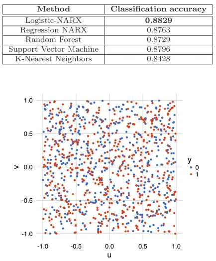
. A total of 1000 input-output data points were collected. Plotting such points produces the figure shown in Fig.1.

Most classification techniques are able to perform static binary classification with high accuracy. We apply our new algorithm to this dataset. The data is separated in a training set (700 points) and a testing set (300 points). Given that this is a static problem, no lags are used, and the nonlinear degree is chosen asℓ= 3, which results in a search space with 10 model terms. Therefore, the maximum number of terms is selected as nmax = 10, and 10 folds are used to compute the cross-validation accuracy. Fig.2 shows the cross-validation

accuracy plot obtained after applying Algorithm1and it suggests that no significant improvement is obtained in accuracy with models that have more than 4 models terms. Therefore, a model with 4 terms is chosen and these are shown in Table1. Such results show that our algorithm was able to identify correctly all model terms involved in the decision boundary for (12). The parameters obtained are log odds ratios, therefore they do not necessarily need to resemble the ones in the decision boundary function.

[image:7.612.212.401.58.230.2] [image:7.612.233.379.278.425.2]

(8)

[image:8.612.251.362.61.118.2]

Table 1 Identified model terms for (12) using Algorithm1

Model Term Parameter

v2₍_k₎ _-12.297

constant 6.459

[image:8.612.198.415.141.403.2]

u2₍_k₎ _-6.632 u2₍_k₎_v₍_k₎ _4.470

Table 2 Comparison of accuracy performance between different methods for modelling of (12)

Method Classification accuracy

Logistic-NARX 0.8829

Regression NARX 0.8763

Random Forest 0.8729

Support Vector Machine 0.8796 K-Nearest Neighbors 0.8428

-1.0 -0.5 0.0 0.5 1.0

u

v y0

1

Fig. 3 Data points obtained from the input-output system given in equation (13)

The results are shown in Table2. It can be seen that our new method has a comparable performance with the rest of the techniques, making it a feasible alternative for static binary classification problems.

4.2 Example 2

Let us consider a slightly different version of equation (12) as follows:

y(k) = ⎧ ⎪ ⎨

⎪ ⎩

1 ifu2(k−1) + 2v2(k−2)

−0.8u2(k−2)v(k−1) +e(k)<1 0 otherwise

(13)

Plotting again the 1000 data points results in the figure shown in Fig.3. As it can be observed, there is not a clear boundary between the two classes as in Fig.1. This is a problem as it can be wrongly suggested that the two classes cannot be separated.

We apply our new algorithm to this dataset. The data is separated in a training set (the first 700 points) and a testing set (the last 300 points). The maximum lags for the inputs and output are chosen to benu=ny = 4,

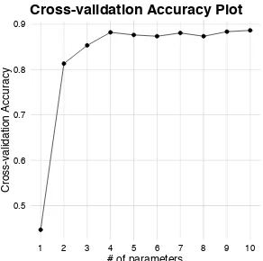
and the nonlinear degree isℓ= 3, which results in a search space with 165 model terms. The maximum number of terms is selected asnmax= 10, and 10 folds are used to compute the cross-validation accuracy. Fig.4shows the

cross-validation accuracy plot obtained after applying Algorithm 1and it suggests that the most parsimonious model with the best accuracy has 4 models terms. These are shown in Table 3. Such results show that our algorithm was able to identify correctly all model terms involved in the decision boundary for (13). Again, the parameters obtained are log odds ratios, therefore they do not necessarily need to resemble the ones in the decision boundary function.

(9)

0.5

0.6 0.7 0.8 0.9

1 2 3 4 5 6 7 8 9 10

# of parameters

C

ro

ss-va

lid

a

ti

o

n

Accu

ra

cy

[image:9.612.234.380.47.192.2]

v2₍_k₋₂₎ _-12.508

constant 6.155

u2₍_k₋₁₎ _-6.086 u2₍_k₋₂₎_v₍_k₋₁₎ _4.582

Random Forest (without autoregressive inputs) 0.5034 Support Vector Machine (without autoregressive inputs) 0.5574 K-Nearest Neighbors (without autoregressive inputs) 0.5267 Random Forest (with autoregressive inputs) 0.8514 Support Vector Machine (with autoregressive inputs) 0.777 K-Nearest Neighbors (with autoregressive inputs) 0.6284

trained with the same training set.In general, traditional classification techniques do not consider lagged variables unless these are explicitly included, thereforetwo cases are considered: the first case assumes that no autoregressive terms are available, therefore onlyu(k)andv(k)are used. In the second one,the same lagged input and output variables that were considered for the logistic-NARX modelare used with the maximum lags chosen to benu= ny = 4(the regression-like NARX model only considers the second

case). All models are compared using the testing set and the OSA accuracy. The results are shown in Table 4. It can be seen that our new method has the best accuracy performance together with the regression-like NARX model. This is expected given the NARX-like structure that generates the data. Nevertheless, the regression-like NARX model produces real-valued outputs, which make them difficult to interpret for classification. On the other hand, the logistic-NARX model is preferred because its outputs are restricted to range from 0 to 1, and they can be used as classification probabilities. Furthermore, the random forest, support vector machine and k-nearest neighbors models are not able to generate reliable results if lagged variables (i.e. values observed in some previous time instants) are not taken into account when defining the feature vector, however their performance is increased when the autoregressive input variables are included. Although it may be argued that our method is just slightly better than the random forest with autoregressive inputs, it must be taken into consideration that the logistic NARX model is transparent and the role or contribution of individual regressors can be known.

4.3 Example 3

Assume we have the following input-output system:

y(k) = ⎧ ⎪ ⎪ ⎪ ⎨

⎪ ⎪ ⎪ ⎩

1 if −u(k−1)1

|v(k−1)|

+0.5u3(k−1)

+ sin (v(k−2)) +e(k)<0 0 otherwise

[image:9.612.238.373.243.298.2] [image:9.612.131.471.327.418.2]

(10)

where the inputsu(k)andv(k)are uniformly distributed between[−1,1], i.e.u(k), v(k)∼U(−1,1), the error sequence is given bye(k) =w(k) + 0.3w(k−1) + 0.6w(k−2)andw(k)is normally distributed with zero mean and variance of 0.01, i.e.w(k)∼N(0,0.01). A total of 1000 input-output data points were collected.

We apply our new algorithm to this dataset. The data is separated in a training set (the first 700 points) and a testing set (the last 300 points). The maximum lags for the inputs and output are chosen to benu=ny = 4,

and the nonlinear degree isℓ= 3, which results in a search space with 165 model terms. The maximum number of terms is selected asnmax= 10, and 10 folds are used to compute the cross-validation accuracy. Fig.5shows the

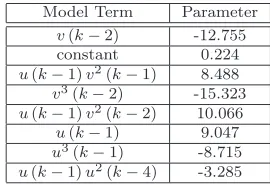
cross-validation accuracy plot obtained after applying Algorithm 1and it suggests that the most parsimonious model with the best accuracy has 8 models terms. These are shown in Table5.

0.875 0.900 0.925 0.950

1 2 3 4 5 6 7 8 9 10

# of parameters

C

ro

ss-va

lid

a

ti

o

n

Accu

ra

cy

[image:10.612.233.379.173.319.2]

v(k−2) -12.755 constant 0.224

u(k−1)v2₍_k₋₁₎ _8.488 v3₍_k₋₂₎ _-15.323 u(k−1)v2₍_k₋₂₎ _10.066 u(k−1) 9.047

u3₍_k₋₁₎ _-8.715 u(k−1)u2₍_k₋₄₎ _-3.285

Similarly to the previous case study, a regression-like NARX model based on the approach suggested in [7], a random forest with 500 trees, a support vector machine with a radial basis kernel, and a k-nearest neighbors model are trained with thesametraining set.Again, twocases are considered: the first case assumes that no autoregressive terms are available, therefore onlyu(k)andv(k)are used. In the second one,the same lagged input and output variables that were considered for the logistic-NARX model are used with the maximum lags chosen to benu=ny= 4, and the nonlinear degree isℓ= 3, which results in a search space with

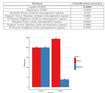
165 model terms. All models are compared using the testing set and the OSA accuracy. The results are shown in Table6. It can be seen that our new method has the best accuracy performance, with a very similar result to the regression-like NARX model and the random forest with autoregressive inputs. Once more, the advantage over the random forest models is the transparency and interpretability about the role or contribution of individual regressors. Also, the advantage over the regression-like NARX model is a more interpretable output that is easily related to a classification probability.

5 Application to Real Data

[image:10.612.237.372.399.493.2]

(11)

[image:11.612.130.475.57.363.2]

Random Forest (without autoregressive inputs) 0.527 Support Vector Machine (without autoregressive inputs) 0.4932 K-Nearest Neighbors (without autoregressive inputs) 0.47

Random Forest (with autoregressive inputs) 0.9223 Support Vector Machine (with autoregressive inputs) 0.8986 K-Nearest Neighbors (with autoregressive inputs) 0.7973

200 200

39 244

0 50 100 150 200 250

Training Testing

Dataset

Cancer

Benign

Malignant

Fig. 6 Frequency of each cancer type for the training and testing sets.

5.1 Breast Cancer Classification

Breast cancer is the most common cancer in women worldwide [56]. Among the different prevention and control techniques, early detection is still the best method in order to improve breast cancer outcome and survival [58]. For this case study, we use the breast cancer dataset from the University of Wisconsin Hospitals, Madison from Dr. William H. Wolberg [57]. This dataset contains 699 instances with the following 10 attributes:

– ID number

– Clump thickness (integer value between 1 and 10)

– Uniformity of cell size (integer value between 1 and 10)

– Uniformity of cell shape (integer value between 1 and 10)

– Marginal adhesion (integer value between 1 and 10)

– Single epithelial cell size (integer value between 1 and 10)

– Bare nuclei (integer value between 1 and 10)

– Bland chromatin (integer value between 1 and 10)

– Normal nucleoli (integer value between 1 and 10)

– Mitoses (integer value between 1 and 10)

– Class (2 for benign, 4 for malignant)

The bare nuclei attribute contains 16 missing values. Such instances were removed from the analysis. Also, the ID number attribute does not provide any meaningful information for the classification task, so it is removed from the dataset. The class attribute is recoded with ’0’ for a benign case and ’1’ for a malignant. The rest of the attributes are divided by 10 in order to have feature values ranging from 0.1 to 1.

The data is separated in a training set (400 instances with 200 samples from each class) and a testing set (283 instances). The frequency of the class for each set is shown in Figure6where it can be noticed that each cancer type has the same frequency in the training set, however, this is not the case in the testing set. Nevertheless, this is not a significant issue as the training phase has access to a good balance of the two classes that need to be identified, while the imbalanced testing set can be used to check the performance of the trained model.

(12)

0.5

5 6 7 9

# of parameters

C

ro

ss-va

lid

a

ti

o

n

Accu

ra

cy

Fig. 7 Cross-validation accuracy plot obtained for the Breast Cancer dataset using Algorithm1

accuracy plot obtained after applying Algorithm1and it suggests that no significant improvement is obtained in accuracy with models that have more than 3 models terms. Therefore, a model with 3 terms is chosen and these are shown in Table7.

Table 7 Identified model terms for the Breast Cancer dataset using Algorithm1

Bare nuclei 6.430

constant -5.774

Uniformity of cell size 11.338

Once more, a regression-like NARX model based on the approach suggested in [7], a random forest with 500 trees, a support vector machine with a radial basis kernel, and a k-nearest neighbors model are trained with the

[image:12.612.232.379.47.195.2]

sametraining set. All models are compared using the testing set and the classification accuracy. The results are shown in Table8. All the methods are able to obtain a good classification accuracy. Although the logistic NARX has not the best accuracy, the difference with the best ones is negligible. This makes the logistic NARX model a competitive alternative to other classification techniques.

Table 8 Comparison of accuracy performance between different methods for modelling of the Cancer Breast dataset

Random Forest 0.9787

Support Vector Machine 0.9681 K-Nearest Neighbors 0.9716

5.2 Electroencephalography Eye State Identification

Recently, electroencephalography eye state classification has become a popular research topic with several appli-cations in areas like stress features identification, epileptic seizure detection, human eye blinking detection, among others [59]. For this case study, we use the EEG Eye State dataset found at the UCI Machine Learning Repos-itory [57]. This dataset contains 14,980 EEG measurements from 14 different variables taken with the Emotiv EEG neuroheadset during 117 seconds. The eye state of the patient was detected with the aid of a camera during the experiment. If the eye is closed, it is coded as a ’1’, otherwise it is coded as ’0’.

For this analysis, the first 80% of the dataset is used for training, while the rest is used for testing. The frequency of the eye state for each dataset is shown in Figure8. Similar to the breast cancer scenario, the two eye states have roughly the same frequency in the training set, however, this is not the case in the testing set. Once more, this is not a significant issue as the training phase can be performed with enough information from both eye states, while the imbalanced testing set can be used to check the performance of the trained model.

[image:12.612.200.415.476.539.2]

(13)

5541 6443

2716

280

0 2000 4000 6000

Training Testing

Dataset

F

re

q

u

e

n

cy

Fig. 8 Frequency of the eye state for the training and testing sets.

with the mean value of the remaining measurements for each variable. The eye state time series, together with the 14 cleaned variables, are shown in Figure 9. Second,an attempt to train a model using the original dataset was done. However, given the high variability and dependency between the variables measured, the model does not perform well enough.Because of this, a principal component analysis (PCA) is performed in order to reduce the dimensionality of both the data and model space, and in this study the 5 most important principal components (PCs) were used to represent the features of the original data. The PC time series are shown in Figure10. Each PC is treated to be a new input variable; lagged PC variables were then used to built a logistic-NARX model. For this analysis, the variables are transformed using scaling, centering and Box-Cox transformations. Therefore, the PCs summarise the main variability of the dataset and simplify the identification process. The preprocessing parameters obtained during the training phases are directly used on the testing set in order to avoid the data snooping problem.

We apply the logistic-NARX modelling approach to this dataset. The output variable is the eye state signal, and the input variables are the 5 PCs computed in the preprocessing phase. For this scenario, no lagged variables of the output signal are used in order to ensure that the model captures a pattern with the exogenous inputs only. The maximum lag for the inputs is chosen to be nu = 50, and the nonlinear

degree isℓ= 1based on the results of previous works in[33,59]. The search space is made up of 251 model terms. The maximum number of terms to look for is chosen asnmax= 30, and 10 folds are used to compute the

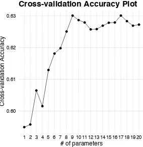
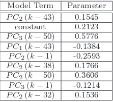
[image:13.612.211.401.52.245.2]

cross-validation accuracy. Fig.11shows the cross-validation accuracy plot obtained after applying Algorithm 1 and it suggests that the most parsimonious model with the best accuracy has 9 models terms. These are shown in Table9.

Table 9 Identified model terms for the EEG Eye State dataset using Algorithm1

P C2(k−43) 0.1545

constant 0.2123

P C3(k−50) 0.5776 P C1(k−43) -0.1384 P C2(k−1) -0.2593 P C2(k−38) 0.1766 P C2(k−50) 0.3606 P C3(k−1) -0.1214 P C2(k−32) 0.1536

[image:13.612.251.362.547.648.2]

(14)

0.0

Eye State

AF3

AF4

F3

F4

F7

F8

FC5

FC6

O1

O2

P7

P8

T7

T8

0 5000 10000 15000

Va

lu

e

[image:14.612.142.481.45.394.2]

Fig. 9 Time series of all variables in the EEG Eye State dataset found at the UCI Machine Learning Repository [57].

Table 10 Comparison of accuracy performance between different methods for modelling of the EEG Eye State dataset

Random Forest (without autoregressive inputs) 0.5475 Support Vector Machine (without autoregressive inputs) 0.6029 K-Nearest Neighbors (without autoregressive inputs) 0.5041 Random Forest (with autoregressive inputs) 0.6365 Support Vector Machine (with autoregressive inputs) 0.6473 K-Nearest Neighbors (with autoregressive inputs) 0.5662

contribute to the classification of the eye state. The models that are trained without autoregressive inputs have a poor classification accuracy. This is improved when autoregressive information is included. However, they do not achieve a classification accuracy like the one obtained by the logistic NARX model.

6 Discussion

[image:14.612.132.477.444.535.2]

(15)

Eye State

PC 1

PC 2

PC 3

PC 4

PC 5

0 5000 10000 15000

0

0 5

0 1 2

Index

Va

lu

[image:15.612.139.479.49.395.2]

e

Fig. 10 Time series of the 5 most important principal components.

0.60 0.61 0.62 0.63

1 2 3 4 5 6 7 8 9 10 11 12 13 14 15 16 17 18 19 20

# of parameters

C

ro

ss-va

lid

a

ti

o

n

Accu

ra

cy

Fig. 11 Cross-validation accuracy plot obtained for the EEG Eye State dataset using Algorithm1

The logistic-NARX model overcomes this by providing variable importance and interpretability about how the variables are interacting. Nevertheless, there are some limitations to the proposed algorithm. First of all, this work focuses on polynomial-like structures, therefore, severe nonlin-earities may not be modeled properly. To overcome this, other structures can be considered (e.g. radial basis functions, wavelets), and this will be considered in a future extension of this work. Another issue, is the selection of the maximum lags for the output and input sequences (ny and

[image:15.612.235.377.433.579.2]

(16)

the performance of the logistic-NARX model can be affected if the data are not balanced (espe-cially when the output data are imbalanced). The scenario of imbalanced data is typical in many real applications where the minority class is dominated or buried by the majority class. Several approaches are available for dealing with imbalanced data problem, readers are referred to [32,60] for details.

7 Conclusion

In this work we developed a novel algorithm that combines logistic regression with the NARX methodology. This allows to tackle classification problems where the output signal is a binary sequence and the regressors are continuous lagged variables. Our approach can deal with the multicollinearity problem while producing models that predicts binary outcomes. From the five case studies, the performance of the proposed logistic NARX models is preferable to that of the other compared methods when dealing with binary-label prediction, where it is sometimes highly desirable to know which input variables play an important role individually and/or interactively in the classification process. The results obtained are promising, and future research may extend this method to multi-class problems.

8 Acknowledgement

The authors acknowledge the financial support to J. R. Ayala Solares from the University of Sheffield and the Mexican National Council of Science and Technology (CONACYT). The authors gratefully acknowledge that part of this work was supported by the Engineering and Physical Sciences Research Council (EPSRC) under Grant EP/I011056/1 and Platform Grant EP/H00453X/1, and ERC Horizon 2020 Research and Innovation Action Framework Programme under Grant No 637302 (PROGRESS).

References

1. S.A. Billings,Nonlinear System Identification: NARMAX Methods in the Time, Frequency, and Spatio-Temporal Do-mains(Wiley, 2013)

2. T. Söderström, P. Stoica,System Identification(Prentice Hall, 1989)

3. K.J. Pope, P.J.W. Rayner, inAcoustics, Speech, and Signal Processing, 1994. ICASSP-94., 1994 IEEE International Conference on, vol. IV (1994), vol. IV, pp. 457 – 460

4. S.A. Billings, S. Chen, R.J. Backhouse, Mechanical Systems and Signal Processing3(2), 123 (1989) 5. S.A. Billings, H.L. Wei, IEEE Transactions on Neural Networks18(1), 306 (2007)

6. H.L. Wei, D.Q. Zhu, S.A. Billings, M.A. Balikhin, Advances in Space Research 40(12), 1863 (2007). URL

http://www.sciencedirect.com/science/article/pii/S0273117707002086

7. S.A. Billings, H.L. Wei, International Journal of Control81(5), 714 (2008)

8. H.L. Wei, S.A. Billings, International Journal of Modelling, Identification and Control3(4), 341 (2008)

9. A.K. Alexandridis, A.D. Zapranis, Neural Networks42(0), 1 (2013). DOI http://dx.doi.org/10.1016/j.neunet.2013.01. 008. URLhttp://www.sciencedirect.com/science/article/pii/S0893608013000129

10. S.A. Billings, H.L. Wei, International Journal of Systems Science36(3), 137 (2005) 11. S.A. Billings, H.L. Wei, Neural Networks, IEEE Transactions on16(4), 862 (2005)

12. H.L. Wei, S.A. Billings, Y. Zhao, L. Guo, Neural Networks, IEEE Transactions on20(1), 181 (2009)

13. S.A. Billings, H.L. Wei, M.A. Balikhin, Neural Networks 20(10), 1081 (2007). URL

http://www.sciencedirect.com/science/article/pii/S0893608007001876

14. D. Koller, M. Sahami, inIn 13th International Conference on Machine Learning(1995)

15. S. Wang, H.L. Wei, D. Coca, S.A. Billings, International Journal of Systems Science44(2), 223 (2013)

16. T. Speed, Science 334(6062), 1502 (2011). DOI 10.1126/science.1215894. URL

http://www.sciencemag.org/content/334/6062/1502.short

17. D.N. Reshef, Y.A. Reshef, H.K. Finucane, S.R. Grossman, G. McVean, P.J. Turnbaugh, E.S. Lander, M. Mitzenmacher, P.C. Sabeti, Science 334(6062), 1518 (2011). DOI 10.1126/science.1205438. URL

http://www.sciencemag.org/content/334/6062/1518.abstract

18. G.J. Székely, M.L. Rizzo, N.K. Bakirov, The Annals of Statistics35(6), 2769 (2007) 19. G.J. Székely, M.L. Rizzo, Journal of Statistical Planning and Inference143(8), 1249 (2013)

20. L. Piroddi, W. Spinelli, International Journal of Control 76(17), 1767 (2003). URL

http://dx.doi.org/10.1080/00207170310001635419

21. J. Ayala Solares, H.L. Wei, Nonlinear Dynamics pp. 1–15 (2015). URLhttp://dx.doi.org/10.1007/s11071-015-2149-3

22. H.L. Wei, S.A. Billings, International Journal of Modelling, Identification and Control5(2), 93 (2008)

23. P. Li, H.L. Wei, S.A. Billings, M.A. Balikhin, R. Boynton, Journal of Computational and Nonlinear Dynamics8(4), 10 (2013)

24. Y. Li, H.L. Wei, S.A. Billings, P. Sarrigiannis, International Journal of Systems Science pp. 1–11 (2015). URL

http://dx.doi.org/10.1080/00207721.2015.1014448

25. Y. Guo, L. Guo, S. Billings, H.L. Wei, International Journal of Systems Science 46(5), 776 (2015). DOI 10.1080/ 00207721.2014.981237. URLhttp://dx.doi.org/10.1080/00207721.2014.981237

26. Y. Guo, L.Z. Guo, S.A. Billings, H.L. Wei, Neurocomputing (2015). URL

(17)

27. G. James, D. Witten, T. Hastie, R. Tibshirani,An Introduction to Statistical Learning with Application in R,Springer Texts in Statistics, vol. 103 (Springer, 2013)

28. F. Harrell,Regression Modeling Strategies: with Applications to Linear Models, Logistic and Ordinal Regression, and Survival Analysis(Springer, 2015)

29. J. Pallant,SPSS Survival Manual (McGraw-Hill Education (UK), 2013)

30. L. Breiman, Machine Learning45(1), 5 (2001). URLhttp://dx.doi.org/10.1023/A%3A1010933404324

31. V.N. Vapnik,Statistical Learning Theory(Wiley, 1998)

32. M. Kuhn, K. Johnson,Applied Predictive Modeling(Springer, 2013)

33. H.L. Wei, S.A. Billings, J. Liu, International Journal of Control77(1), 86 (2004)

34. M.T. Rashid, M. Frasca, A.A. Ali, R.S. Ali, L. Fortuna, M.G. Xibilia, Nonlinear Dynamics69(4), 2237 (2012). DOI 10.1007/s11071-012-0422-2. URLhttp://dx.doi.org/10.1007/s11071-012-0422-2

35. H. Wickham, G. Grolemund,R for Data Science (O’Reilly Media, 2016)

36. L.A. Aguirre, C. Jácôme, in Control Theory and Applications, IEE Proceedings-, vol. 145 (IET, 1998), vol. 145, pp. 409–414

37. B. Feil, J. Abonyi, F. Szeifert, Journal of Process Control14(6), 593 (2004)

38. S.L. Kukreja, J. Lofberg, M.J. Brenner, inSystem Identification, vol. 14 (2006), vol. 14, pp. 814–819

39. P. Qin, R. Nishii, Z.J. Yang, Nonlinear Dynamics 70(3), 1831 (2012). DOI 10.1007/s11071-012-0576-y. URL

http://dx.doi.org/10.1007/s11071-012-0576-y

40. H. Zou, T. Hastie, Journal of the Royal Statistical Society: Series B (Statistical Methodology)67(2), 301 (2005) 41. X. Hong, S. Chen, in16th IFAC Symposium on System Identification(2012), pp. 1814–1819

42. S. Sette, L. Boullart, Engineering Applications of Artificial Intelligence14(6), 727 (2001)

43. J. Madár, J. Abonyi, F. Szeifert, Industrial & Engineering Chemistry Research44(9), 3178 (2005) 44. T. Baldacchino, S.R. Anderson, V. Kadirkamanathan, Automatica48(5), 857 (2012)

45. B.O. Teixeira, L.A. Aguirre, Journal of Process Control21(1), 82 (2011) 46. S.A. Billings, W.S.F. Voon, International Journal of Control44(1), 235 (1986)

47. T.G. Dietterich, inStructural, Syntactic, and Statistical Pattern Recognition(Springer, 2002), pp. 15–30 48. L.A. Aguirre, C. Letellier, Mathematical Problems in Engineering2009(35) (2009)

49. H.L. Wei, M.A. Balikhin, S.N. Walker, inComputer Science & Education (ICCSE), 2015 10th International Conference on(IEEE, 2015), pp. 125–130

50. S. Billings, K. Mao, Model identification and assessment based on model predicted output. Tech. rep., Department of Automatic Control and Systems Engineering, The University of Sheffield, UK (1998)

51. E.G. Nepomuceno, S.A.M. Martins, Systems Science & Control Engineering4(1), 50 (2016). DOI 10.1080/21642583. 2016.1163296. URLhttp://dx.doi.org/10.1080/21642583.2016.1163296

52. S. Chen, S. Billings, W. Luo, International Journal of Control50(5), 1873 (1989)

53. P. Komarek, Logistic regression for data mining and high-dimensional classification. Master’s thesis, Robotics Institute - School of Computer Science, Carnegie Mellon University, USA (2004)

54. A. Senawi, H.L. Wei, S.A. Billings, Pattern Recognition (2017). Accepted

55. K.P. Bennett, O.L. Mangasarian, Optimization methods and software1(1), 23 (1992) 56. O.L. Mangasarian, W.N. Street, W.H. Wolberg, Operations Research43(4), 570 (1995) 57. M. Lichman. UCI Machine Learning Repository (2013). URLhttp://archive.ics.uci.edu/ml

58. WHO. Breast cancer: prevention and control. URLhttp://www.who.int/cancer/detection/breastcancer/en/

59. T. Wang, S.U. Guan, K.L. Man, T.O. Ting, Mathematical Problems in Engineering2014(2014)