This is a repository copy of
Robust Bayesian Filtering Using Bayesian Model Averaging
and Restricted Variational Bayes
.
White Rose Research Online URL for this paper:
http://eprints.whiterose.ac.uk/131390/
Version: Accepted Version
Proceedings Paper:
Khalid, S., Rehman, N.U., Abrar, S. et al. (1 more author) (2018) Robust Bayesian Filtering
Using Bayesian Model Averaging and Restricted Variational Bayes. In: Proceedings of the
International Conference on Information Fusion. International Conference on Information
Fusion, 10-13 Jul 2018, Cambridge, UK. IEEE . ISBN 978-0-9964527-6-2
10.23919/ICIF.2018.8455608
[email protected] https://eprints.whiterose.ac.uk/ Reuse
Items deposited in White Rose Research Online are protected by copyright, with all rights reserved unless indicated otherwise. They may be downloaded and/or printed for private study, or other acts as permitted by national copyright laws. The publisher or other rights holders may allow further reproduction and re-use of the full text version. This is indicated by the licence information on the White Rose Research Online record for the item.
Takedown
If you consider content in White Rose Research Online to be in breach of UK law, please notify us by
Robust Bayesian Filtering Using Bayesian Model
Averaging and Restricted Variational Bayes
S. S. Khalid, N. U. Rehman
EE Department, COMSATS Instituteof Information Technology Islamabad, Pakistan
{safwan khalid,naveed.rehman}
@comsats.edu.pk
Shafayat Abrar
School of Science and Engineering Habib University, Karachi, Pakistan [email protected]
Lyudmila Mihaylova
Department of Automatic Control and Systems EngineeringThe University of Sheffield, UK [email protected]
Abstract—Bayesian filters can be made robust to outliers if the solutions are developed under the assumption of heavy-tailed distributed noise. However, in the absence of outliers, these robust solutions perform worse than the standard Gaussian assumption based filters. In this work, we develop a novel robust filter that adopts both Gaussian and multivariate t-distributions to model the outliers contaminated measurement noise. The effects of these distributions are combined within a Bayesian Model Averaging (BMA) framework. Moreover, to reduce the computational com-plexity of the proposed algorithm, a restricted variational Bayes (RVB) approach handles the multivariate t-distribution instead of its standard iterative VB (IVB) counterpart. The performance of the proposed filter is compared against a standard cubature Kalman filter (CKF) and a robust CKF (employing IVB method) in a representative simulation example concerning target tracking using range and bearing measurements. In the presence of outliers, the proposed algorithm shows a 38% improvement over CKF in terms of root-mean-square-error (RMSE) and is computationally 2.5times more efficient than the robust CKF.
I. INTRODUCTION
Target tracking deals with the estimation of unknown states, such as position, velocity and acceleration of a moving tar-get, using noisy measurements in a given coordinate space. Algorithms that can accurately track the mobility of a target offer numerous advantages in a wide range of applications. The most obvious example is tracking an aircraft using radar measurements. It is of immense importance in many military applications and is also essential for air traffic control required by civilian airlines. Some other examples include tracking of a mobile node in a cellular network which is required for effi-cient radio resource management and tracking in autonomous cars and robots. Target tracking algorithms, despite having a diverse range of applications, employ a common structure based on the Bayesian filtering framework for extracting useful information from the available data. The standard Bayesian filtering solutions such as traditional Kalman filters (in case of linear systems) and sigma-point filters (e.g., Cubature Kalman Filter (CKF), Unscented Kalman Filter (UKF), etc., for nonlinear systems), assume that the noises have Gaussian distribution [1]. In practice, however, large deviations (outliers) occur in real data frequently and these cannot be modeled accurately by a Gaussian distribution only [2]. As a result,
filters relying on the Gaussian assumption do not perform well when outliers are present[3].
A Bayesian filter can be made robust to outliers if the Gaussian assumption is dropped in favor of a heavy-tailed distribution. A suitable choice is the use of multivariate gener-alization of Studentt-distribution [2–8]; hereafter, referred to as t-distribution. However, the incorporation of t-distributed uncertainties in a Bayesian framework is not trivial as the required posterior probability becomes intractable. Recently, a number of works [2, 5, 6, 9] have advocated the use of variational Bayes (VB) framework to handle t-distributed measurement noise in Bayesian filters. In the VB method, a solution is obtained by approximating the intractable posterior probability density function into a tractable factored form. These state-of-the-art robust solutions, however, suffer from two drawbacks: 1) The standard application of the VB method results in an iterative procedure (IVB) that requires a number of fixed-point iterations to converge to an admissible inference. These iterations, though few in number (usually four or five), may become prohibitive in real-time applications due to the involvement of matrix inversion operations; 2) The resulting solutions though indeed robust to outliers, do not perform well in the absence of outliers, as compared to the conventional filters based on Gaussian assumption.
In this work, we propose a filter able to deal with both these challenges by,
1) Adopting a restricted VB (RVB) approach to get rid of the iterative procedure, and develop an approximate computationally-efficient recursive solution for Bayesian filtering undert-distributed measurement noise. 2) Instead of modeling the observation noise using a
sin-gle t-distributed process, we advocate the use of two separate models, one Gaussian distributed and one t -distributed. The proposed filter then combines these two models using a Bayesian Model Averaging (BMA) [7] approach.
this work, the proposed BMA-RVB method can easily be com-bined with sigma-point methods to develop computationally efficient robust solutions for nonlinear systems. The rest of this paper is organized as follows: in Section II, we describe the system models and develop the proposed filtering algorithm. In section III, we present simulation results and in Section IV, we draw conclusions.
A. Notations
We represent scalers using small letters. Column vectors denoting states and measurements are represented by bold-faced small letters. Matrices are represented using bold-bold-faced capital letters. A set of column vectors is also represented using bold-faced capital letters. We use In to denote an n× n identity matrix. We use T in superscript to represent the transpose operation of a matrix. A variablexthat is distributed according to t-distribution is denoted asx∼St(µ,Σ, η), i.e.,
p(x) = Γ((η+d)/2) Γ(η/2)
1 (ηπ)d/2√Σ
1 +δ
2(x)
η
−(η+d)/2
,
where δ2(x) = (x
−µ)TΣ−1(
x−µ), d = dim(x), µ is the mean, η is the degree-of-freedom parameter, andΣis the
scale matrix of the p(x).
Note that η is a shape parameter that determines tail-behavior [11]. Heavier tails are obtained when η is close to one. Conversely, for larger values of η, p(x) approaches the standard normal distribution. Also note that t-distribution has infinite variance for η < 2; therefore, throughout this work, we shall assume thatη >2. Finally, the covariance matrix of
x∼St(µ,Σ, η)is given by η
η−2Σ for η >2.
II. SYSTEMMODEL ANDPROPOSEDALGORITHM
Let us consider the following dynamic system:
xk =f(xk−1) +wk, (1a)
yk =h(xk) +vk, (1b)
where xk ∈ Rn is the dynamic state vector, yk ∈ Rm is the observation vector, f(·) and h(·) are arbitrary nonlinear functions, wk ∼ N(0;Q
k) models the uncertainties in the
system model andvk is the outliers contaminated observation noise. To account for the effects of the outliers, we model
vk as a combination of a Gaussian and at-distribution. The transition between these two distributions is governed by a first-order jump Markovian process sk that can take two
possible values s1 and s2, i.e., vk(sk=s1) ∼ N(0;Rk) and v(sk=s2)
k ∼St(0;Σk;η), whereΣk =η−η2Rk. Hereafter, we
use the notations(ki)to denotesk=sifori= 1,2. We assume
that the transition probabilities p(s(ki)|sk(j−)1) =πji are known
a priori. Note that the noise sequences, {wk} and{vk}, are assumed to be independent for each k.
Let Yk := {y1,y2,· · · ,yk} be the set of all available
observations at instant k; the task of a Bayesian filtering algorithm is to recursively evaluate an estimate of the state
vector xkˆ |k = E[xk|Yk] =
R
xkp(xk|Yk)dxk1. Noting that
at any instant, the observation noisevk may belong to one of the two possible models, we expandp(xk|Yk)as follows:
p(xk|Yk) =
2
X
i=1
p(xk|Yk, s(ki))
| {z }
Posterior
p(s(ki)|Yk)
| {z }
Weighting Factor
. (2)
Using Bayes theorem, p(xk|Yk, s(ki)) can be written as a
product of alikelihood and apredictiondensity, as follows:
p(xk|Yk, s(1ki))∝p(yk|xk,Yk−1, s(ki))
| {z }
likelihood
p(xk|Yk−1, s(ki))
| {z }
Prediction .
(3) In the following, we derive expressions for the evaluation of
prediction,likelihood,posterior, and theweighting factor. We discuss how the required probability p(xk|Yk) is
approxi-mated at each instant k and also discuss the computational cost of the resulting algorithm.
A. Prediction
Let us first consider the evaluation of prediction density. By introducing marginalization overxk−1, we can write
p(xk|Yk−1, s(ki)) =
Z
p(xk|xk−1,Yk−1, s(ki))×
p(xk−1|Yk−1, s(ki))dxk−1
=
Z
p(xk|xk−1)p(xk−1|Yk−1)dxk−1, (4) where we have used the fact that the probability of xk
is completely specified given xk−1 and the value of sk at kth instant does not affect the probability of xk−1. Ac-cordingly, the prediction density is independent of the value of s(ki), i.e., p(xk|Yk−1, s(ki)) = p(xk|Yk−1). In BMA framework, we assume that p(xk−1|Yk−1) is approximated using a single Gaussian distribution, i.e., p(xk−1|Yk−1) ≈
Nxk−1(ˆxk−1|k−1;Pk−1|k−1), wherexˆk−1|k−1andPk−1|k−1 are known from previous recursion. Also, from (1a), we note that p(xk|xk−1) = Nxk(f(xk−1);Qk). To derive a
closed-form expression for (4), we still require to linearize the nonlinear function f(·). To achieve this result, we apply statistical linear regression (SLR) [12, 13] on f(xk−1) as follows:
f(xk−1)≈Fk−1xk−1+bk−1+efk−1, (5)
where Fk−1 ∈ Rn×n, bk−1 ∈ Rn are to be determined and efk−1 is the linearization error that is assumed to be a zero-mean Gaussian distributed process with covariance equal to Ωf
k−1. We also assume that e
f
k−1 is independent from
xk−1 and wk. Note that bk−1 is introduced to make the approximation in (5) unbiased, we evaluatebk−1 as
bk−1= E[f(xk−1)−Fk−1xk−1|Yk−1]
= ¯xk|k−1−Fk−1xˆk−1|k−1,
(6)
where
¯
xk|k−1=
Z
f(xk−1)p(xk−1|Yk−1)dxk−1. (7)
Now, from (5), the linearization error can be written asefk−1≈ f(xk−1)−Fk−1xk−1−bk−1. The value ofFk−1is evaluated by minimizing the mean square of this linearization error, i.e.,
F†k−1= argmin
F
E[(f(xk−1)−Fk−1xk−1−bk−1)T×
(f(xk−1)−Fk−1xk−1−bk−1)|Yk−1]
= E
(f(xk−1)−xk¯ −1)−Fk−1(xk−1−xˆk−1|k−1) ×
(f(xk−1)−xk¯ −1)−Fk−1(xk−1−xkˆ −1|k−1)
T |Yk−1
.
(8) Let us define Pxfk−1 := E[(xk−1 −xkˆ −1|k−1)(f(xk−1)−
¯
xk|k−1)T|Yk−1], then taking the derivative of (8) with respect toFk−1 and setting it to zero, we get
F†k−1= (Pxfk−1)TP−1
k−1|k−1. (9)
In the following, we simply use Fk−1 instead of F†k−1, to keep the notation simple. Using the expression for Fk−1, the covariance matrix of efk−1 is evaluated as
Ωf
k−1:= E[e
f k−1(e
f k−1)
T |Yk−1]
=Pf fk−1−Fk−1Pk−1|k−1FTk−1,
(10)
where
Pf fk−1:=
Z
(f(xk−1)−xk¯ |k−1)×
(f(xk−1)−xk¯ |k−1)Tp(xk−1|Yk−1)dxk−1. (11) Inserting (5) in (1a), we can write
xk≈Fk−1xk−1+bk−1+efk−1+wk. (12)
Consequently, we can approximate p(xk|xk−1) ≈
Nxk(Fk−1xk−1 + bk−1;Qk + Ω f
k−1). Accordingly, the expression in (4) becomes
p(xk|Yk−1, s(1)k )≈
Z
Nxk(Fk−1xk−1+bk−1;Qk+Ω f k−1)
Nxk−1(ˆxk−1|k−1;Pk−1|k−1)dxk−1. (13) To develop a closed-form expression of (13) we require the following theorem:
Theorem 1 (Gaussian Product Theorem [14]):Letx1,µ1∈
Rn, H ∈ Rm×n,x2 ∈ Rm andP1,P2 be positive definite matrices, then
Nx2(Hx1;P2)Nx1(µ1;P1) =Nx2(Hµ1;P3)Nx1(µ;P),
where P3 = HP1HT +P2, µ = µ1 +K(x2−Hµ1),
P =P1−KHP1 andK=P1HTP−31.
Applying Gaussian Product Theorem (GPT) on (13), we get
p(xk|Yk−1)≈
Z
Nxk(Fk−1xkˆ −1|k−1+bk−1;Pk|k−1)×
Nxk−1(µk;Pk)dxk−1 =Nxk(ˆxk|k−1;Pk|k−1),
(14) where xkˆ |k−1 = Fk−1xkˆ −1|k−1 + bk−1 = ¯xk|k−1 and
Pk|k−1=Fk−1Pk−1|k−1FTk−1+Qk+Ω f k−1=P
f f k−1+Qk.
B. Likelihood
The expressions for likelihood can be found from (1b). Firstly, we note that p(yk|xk,Yk−1, s(ki)) = p(yk|xk, s
(i)
k ).
Now, when sk = s1 (i.e., vk is Gaussian), we have
p(yk|xk, s
(1)
k ) = Nyk(h(xk);Rk). Similarly, for sk = s2 (i.e., vk is t-distributed), we have p(yk|xk, s
(2)
k ) =
St(h(xk);Σk;η)
C. Posterior
From (3), we note that the posterior probability density function is proportional to the product of likelihood and prediction densities. Since the expression for likelihood is dependent ons(ki); therefore, we evaluatep(xk|Yk, s(ki))
sep-arately for i= 1andi= 2, in the following:
For sk =s1:
p(xk|Yk, s(1)k )∝ Nyk(h(xk);Rk)Nxk(ˆxk|k−1;Pk|k−1).
(15) To apply GPT on (15), we first linearizeh(xk). We apply SLR onh(xk), as follows:
h(xk)≈Hkxk+ck+ehk. (16)
Using a procedure, similar to that outlined above, forf(xk−1), we getck= ¯yk|k−1−Hkxkˆ |k−1, where
¯
yk|k−1=
Z
h(xk)p(xk|Yk−1)dxk. (17)
Also,Hk = (Pxhk )TP−k|1k−1, where
Pxhk =
Z
(xk−xˆk|k−1)(h(xk)−y¯k|k−1)Tp(xk|Yk−1)dxk, (18)
Phhk =
Z
(h(xk)−y¯k|k−1)(h(xk)−y¯k|k−1)Tp(xk|Yk−1)dxk. (19) The linearization error ehk is assumed to be Gaussian dis-tributed with zero mean and covariance equal to Ωhk, where Ωhk =Phhk −HkPk|k−1HTk. Inserting (16) in (1b), we get a
linearized observation model as follows:
Consequently,p(yk|xk, s
(1)
k )≈ Nyk(Hkxk+ck;Ωhk+Rk).
Inserting (20) in (15) and applying GPT, we get
p(xk|Yk, s(1)k )
∝ Nyk(Hkxk+ck;Ωhk+Rk)Nxk(ˆxk|k−1;Pk|k−1) ∝ Nyk(Hkxkˆ |k−1+ck;HkPk|k−1HTk +Rk+Ωhk)×
Nxk(ˆx
(1)
k|k;P
(1)
k|k).
(21) Note thatNyk(Hkxkˆ |k−1+ck;HkPk|k−1HTk+Rk+Ωhk)is
a term independent of xk; hence, droppingNyk(·,·)in (21),
we obtain p(xk|Yk, s(1)k ) =Nxk(ˆx
(1)
k|k;P
(1)
k|k), where
ˆ
x(1)k|k = ˆxk|k−1+K (1)
k (yk−Hkxˆk|k−1−ck)
= ˆxk|k−1+K (1)
k (yk−y¯k|k−1),
(22)
the expression for K(1)k is given as
K(1)k =Pk|k−1HTk(HkPk|k−1HTk +Ωhk+Rk)−1
=Pxhk (Phhk +Rk)−1, (23)
and the termP(1)k|k can be evaluated as
P(1)k|k=Pk|k−1−K(1)k HkPk|k−1
=Pk|k−1−Pxhk (Phhk +Rk)−1(Pxhk )T.
(24)
For sk =s2:
Similar to the previous case, we write
p(xk|Yk, s(2)k )∝p(yk|xk, s
(2)
k )p(xk|Yk−1)
∝St(h(xk);Σk;η)p(xk|Yk−1). (25)
By introducing a Gamma distributed auxiliary variable λk ∼
Gλk( η
2,
η
2), the density p(yk|xk, s
(2)
k ) may be expressed as
[2]:
p(yk|xk, s(2)k ) =
Z
p(yk|xk, s(2)k , λk)p(λk)dλk, (26)
wherep(yk|xk, s
(2)
k , λk) =Nyk(h(xk);λ1 k
Σk). Furthermore,
the joint density p(xk, λk|Yk, s(2)k )may be expressed as:
p(xk, λk|Yk, sk(2))∝p(yk|xk, s
(2)
k , λk)p(xk|Yk−1)p(λk)
=Nyk h(xk), λ−k1Σk
Nxkxkˆ |k−1,Pk|k−1
Gλk η 2, η 2 , (27) where we exploit the facts that p(xk|λk,Yk−1) =
p(xk|Yk−1)andp(λk|Yk−1) =p(λk). Note that the required
posterior densityp(xk|Yk, s(2)k )can be evaluated by
marginal-izing (27) over λk. To make this tractable, we approximate p(xk, λk|Yk, s(2)k ) as a product of two independent factors,
i.e., p(xk, λk|Yk, s(2)k ) ≈ f1(xk|Yk, s2k)f2(λk|Yk). In the
VB framework,f1(·)andf2(·)are determined by minimizing Kullback-Leibler (KL) divergence between the true and the approximate posteriors. If no fixed functional form is assumed for f1(·) and f2(·) then minimizing KL divergence results in coupling of moments of f1(·) and f2(·). Consequently, a number of fixed-point iterations are required to arrive at
a solution (refer to iterative solutions in [2, 15]). These iterations, however, may be avoided if a fixed functional form is imposed on one of the distributions (say, as in our case,
f2(λk|Yk)). The other factor (i.e., f1(xk|Yk)) can then be
evaluated using the following proposition:
Proposition 1 ([15]): Let f(θ|Y) be the posterior dis-tribution of multivariate parameter θ, where the latter is partitioned into two sub-vectors of parameters,θ= [θ1t,θ2t]t.
Let fb(θ|Y) be an approximation of f(θ|Y) of the kind
b
f(θ|Y) =fb(θ1|Y)fb(θ2|Y), where fb(θ2|Y) be a posterior distribution ofθ2of fixed functional form. Then, the minimum KL divergence, i.e., KL(fb(θ|Y)||f(θ|Y)), is reached for
b
f(θ1|Y)∝exp Efb(θ2|Y)[ln(f(θ|Y))]
.
While the proposition is valid for anyfb(θ2|Y), the choice of the functional form, however, greatly affects the accuracy of the resulting algorithm. Owing to [15], a reasonable choice is to select the exact marginal distribution of the joint posterior, i.e., using (27)
p(λk|Yk)∝
Z
Nyk h(xk), λ−k1Σk
Nxk xkˆ |k−1,Pk|k−1
×
Gλk η
2,
η
2
dxk.
(28) However, the exact marginal in (28) does not yield a tractable form. On the other hand, if we replaceNxk(xkb |k−1,Pk|k−1)
in the marginalization integral by its certainty equivalence approximation [16], i.e.,δ(xk−xkb |k−1), whereδ(·)denotes the Dirac delta function, then the resulting posterior becomes Gamma distributed; this is shown below:
f2(λk|Yk)∝
Z
Nyk h(xk), λ−k1Σkδ xk−xbk|k−1
×
(29a)
Gλk η
2,
η
2
dxk (29b)
=Nyk h(xbk|k−1), λ−k1Σk
Gλk η 2, η 2 (29c) ∝λ η+m
2 −1
k exp −
λk
2 ǫtkΣ−k1ǫk+η
, (29d)
∝Gλk
1 2 η+m
,12 ǫtkΣ−k1ǫk+η
(29e)
whereǫk =yk−h(xkb |k−1). The primary motivation behind using the certainty equivalence approximation is that the resulting posterior f2(λk|Yk) has the same functional form
(i.e., Gamma distribution) as that of the optimal VB-posterior (refer to [2, eq (2)]). Next we apply the aforementioned proposition to determine f1(xk|Yk), i.e., f1(xk|Yk) ∝
exp Ef2(λk|Y)[ln(p(xk, λk|Y))]
; we evaluate
Ef2(λk|Y)[ln(p(xk, λk|Y))] =
−1
2(xk−xkb |k−1)
TP−1
k|k−1(xk−xkb |k−1)
−1
2λ¯k(yk−h(xk))TΣ
−1
k (yk−h(xk)) +C,
(30)
whereC represents those terms which are independent ofxk, andλ¯k := η+m
/ ǫTkΣ−1
k ǫk+η
The argument (30) is quadratic inxk, and this is desirable for obtaining a closed-form solution. Further, we evaluate
f1(xk|Yk, s(2)k )∝exp Ef2(λk|Y)[ln(p(xk, λk|Y))]
∝ Nxk xkb |k−1,Pk|k−1
Nyk h(xk),λ¯−k1Σk.
(31) Now using the linearization of h(xk) as described in (16), we approximate Nyk h(xk),λ¯−k1Σk
≈ Nyk Hkxk +
ck,λ¯−k1Σk+Ωhk. Consequently,
f1(xk|Yk, s(2)k )∝Nxk xkb |k−1,Pk|k−1
× Nyk Hkxk+ck,λ¯k−1Σk+Ωhk
. (32)
Note that (32) is similar to (21) with the only differ-ence that Rk is replaced with ¯λ−k1Σk; accordingly, we get
f1(xk|Yk, s(2)k )≈ Nxk(xb
(2)
k|k;P
(2)
k|k), where
b
x(2)k|k=xbk|k−1+K (2)
k (yk−y¯k|k−1), (33a)
K(2)k =Pxhk (Phhk + ¯λ−k1Σk)−1, (33b) P(2)k|k=Pk|k−1−Pxhk (Phhk + ¯λ−k1Σk)
−1(Pxh
k )T. (33c)
Remark 1: Note that if λ¯k is known, then
the variational Bayes approximation of (32) is
equivalent to approximating the likelihood as
p(yk|xk, s(2)k ) ≈ Nyk Hkxk + ck,¯λ−k1Σk + Ωhk
. We use this approximation in the evaluation of the weighting factorp(s(2)k |Yk), in the next section.
Remark 2: Note that the evaluation of xkˆ |k−1, Pk|k−1 and consequently xˆ(ki|)k, Kk(i) and Pk(i|)k, for i = 1,2, requires the evaluation of moment integrals x¯k|k−1, Pf fk−1,
¯
yk|k−1, Pxhk and Phhk using (7) (11), (17), (18) and
(19), respectively. All these integrals are of the form
I(s) =Rs(x)Nx(ˆx;P)dx, for some nonlinear function s(·).
The integral I(s), in general, does not admit a closed-form solution. However, a large number of numerical integration techniques have been suggested in literature to approximate such integrals [1, and references therein], [17, 18] etc. In this work, we shall employ the third degree cubature rules [17, 19], to approximate the required moment integrals. First, a change of variable is introduced to convert the non-standard Gaussian density, in the integral, into a standard one. Let x = ˆx+√P c, where P = √P√PT
[1]; then, the Gaussian weighted integral is written as
R
s(ˆx+ √P c)Nc(0,I)dc = R
g(c)Nc(0,I)dc =: I(g),
where g(c) := s(ˆx +√P c). Note that √P is a lower triangular matrix obtained from the Cholesky decomposition of P. Now we approximate I(g) using the third-degree cubature method as follows [19, eq (45)]:
I(g) =
Z
g(c)Nc(0,I)dc≈
1 2n
n
X
j=1
[g(√nej) +g(−√nej)],
(34) whereejis an n-dimensional unit vector in thejth-coordinate.
D. Weighting Factor
We now consider the evaluation of the weighting factor
p(s(ki)|Yk)and denote it withµ(ki); we note that
p(s(ki)|Yk) =µ(ki)∝p(yk|s
(i)
k ,Yk−1)p(s
(i)
k |Yk−1). (35)
The second factor in (35), i.e., p(s(ki)|Yk−1) is expanded as follows:
p(s(ki)|Yk−1) = 2
X
j=1
p(s(ki)|sk(j−)1,Yk−1)p(sk(j−)1|Yk−1)
=
2
X
j=1
πjiµ(kj−)1.
(36)
Note that πji is known a priori and µ(kj−)1 is available from the previous recursion. The first factor in (35), i.e.,
p(yk|s
(i)
k ,Yk−1)can be written as
p(yk|s
(i)
k ,Yk−1) =
Z
p(yk|xk, s
(i)
k )p(xk|Yk−1)dxk (37)
Again, we evaluate p(yk|s
(i)
k ,Yk−1)separately for i= 1,2, in the following:
For sk =s1:
p(yk|s
(1)
k ,Yk−1)
≈ Z
Nyk(Hkxk+ck;Ωhk+Rk)Nxk(ˆxk|k−1;Pk|k−1)dxk
=
Z
Nyk(Hkxkˆ |k−1+ck;HkPk|k−1HTk +Rk+Ωhk) Nxk(ˆxk|k;Pk|k)dxk
=Nyk(Hkxˆk|k−1+ck;HkPk|k−1HTk +Rk+Ω h k) = Λ
(1)
k ,
(38) where the last equality in (38) is owing to GPT; also note that
Hkxkˆ |k−1+ck= ¯yk|k−1 andHkPk|k−1HTk +Rk+Ωhk = Phhk +Rk, henceΛ(1)k =Nyk(¯yk|k−1;Phhk +Rk).
For sk =s2:
Employing the approximation suggested in Remark 1, i.e.,
p(yk|xk, s(2)k ) ≈ Nyk Hkxk +ck,λ¯−k1Σk +Ωhk
, we can write
p(yk|s
(2)
k ,Yk−1)≈
Z
Nyk(Hkxk+ck;Ωkh+ ¯λ−k1Σk)× Nxk(ˆxk|k−1;Pk|k−1)dxk
=Nyk(¯yk|k−1;P
hh
k + ¯λ−k1Σk) = Λ(2)k .
(39) Finally, an overall expression for µ(ki) may be written as
µ(ki)=1
cΛ
(i)
k
2
X
j=1
πjiµ(kj−)1, (40)
where c = P2l=1Λ (l)
k
P2
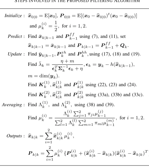
TABLE I
STEPS INVOLVED IN THEPROPOSEDFILTERINGALGORITHM
Initialize: xb0|0= E[x0],P0|0= E[(x0−xb0|0)t(x0−xb0|0)]
andµ(ki)= 1
2,fori= 1,2.
Predict: Findx¯k|k−1andPf fk−1using (7), and (11), set
b
xk|k−1= ¯xk|k−1andPk|k−1=Pf fk−1+Qk.
Update: Findy¯k|k−1,Pxhk andPhhk ,using (17), (18) and (19).
Findλ¯k=
η+m
ǫT kΣ
−1
k ǫk+η
,ǫk=yk−h(xbk|k−1),
m= dim(yk).
FindK(1)k ,bx(1)k|kandP(1)k|kusing (22), (23) and (24).
FindK(2)k ,bx(2)k|kandP(2)k|kusing (33a), (33b) and (33c).
Averaging: FindΛ(1)k , andΛ(2)k , using (38) and (39).
Findµ(ki)= Λ
(i)
k P2
j=1πjiµ( j)
k−1
P2
l=1Λ (l)
k P2
m=1πmlµ(km−)1
, fori= 1,2.
Outputs: xbk|k=
2
X
i=1
b
x(ki|)kµ(ki),
Pk|k=
2
X
i=1
µ(ki){P(ki|)k+ (xb(ki|)k−bxk|k)(xb
(i)
k|k−bxk|k)T}.
E. Approximation
From (3), we note that the required probability p(xk|Yk)
is actually a sum of two weighted densities. However, in the BMA framework, p(xk|Yk) is approximated using a
single Gaussian density at each instant k. Accordingly, we approximate p(xk|Yk) ≈ Nxk(ˆxk|k;Pk|k), where xkˆ |k and Pk|k are obtained by matching moments as follows:
b
xk|k =
2
X
i=1
b
x(ki|)kµ(ki),
Pk|k =
2
X
i=1
µ(ki){P
(i)
k|k+ (xb
(i)
k|k−bxk|k)(bx
(i)
k|k−xbk|k)T}.
(41) This completes our derivation of the proposed filter; based on this derivation, an algorithm is summarized in Table I.
F. Computational Complexity
The asymptotic complexity of the various operations in-volved in the proposed algorithm is listed in Table II. Note that we have usedCf andChto denote the complexity of
eval-uating nonlinear functions f(·) and h(·), respectively. Also,
n= dim{xk}andm= dim{yk}. We note that, for largen,
the time complexity will be dominated by O(n3)operations. However, if either Cf or Ch is greater thanO(n2), then time
complexity will chiefly depend upon function evaluations. Also note that, some operations such asK(ki),xˆ(ki|)k andP(ki|)k
are evaluated for i= 1,2 in the proposed method. Whereas, these operations are performed only once in a standard CKF. Also, the covariance mixing step in the output is owing to model averaging and is not required in standard filters. Hence,
TABLE II
ASYMPTOTIC COMPUTATIONAL COMPLEXITY OF THE VARIOUS STEPS IN PROPOSED ALGORITHM.
Operations ComplexityO(·)
Sigma Points n3 Evaluation off(·),h(·) nCf,nCh b
x|k−1 n2
¯
yk|k−1 nm
Pk|k−1 n3
K(ki) nm2+m3
ˆ
x(ki|)k n2m
P(ki|)k nm2+n2m
Pk|k n2
the complexity of the proposed algorithm is slightly greater than that of standard CKF. However, for large n, both scale according to eitherO(n3). Also, in an iterative VB procedure, all of these operations (apart from covariance mixing) are performed Nitr times, whereNitr is the number of iterations required by the IVB filter to converge. Hence for Nitr >2, the proposed algorithm will always be computationally more efficient than its IVB based counterparts.
III. SIMULATIONRESULTS
In this section, we the performance of the proposed al-gorithm is compared against a conventional CKF [17] and a robust (to outliers) CKF that utilizes iterative variational Bayes (IVB) technique to handle outliers [2, 5], using a simulation example that considers target tracking based on range and bearings measurements. We consider the cases of Gaussian-only as well as Gaussian-with-outliers observation noise models. The root-mean-square-error (RMSE) is used as a figure-of-merit to compare the performance of the various filters.
Let us consider a target that is moving with nearly constant velocity [20], i.e.,
xk=F xk−1+wk, (42)
wherexk= [ζk,ζ˙k, ǫk,ǫ˙k]T,F =F1⊗I2,[ζk, ǫk]denote the
position coordinates; whereas, ζ˙k and ǫ˙k denote velocities in
ζ and ǫdirections, respectively. We have F1 =
1 T
0 1
and
the sampling timeT is set to0.5sec. The uncertainty wk ∼ N(0;Q), where Q = (Q
1⊗I2)σw2, Q1 =
T4/4 T3/2
T3/2 T2
andσw= 2 m/s2. The observation model is specified as
yk =
" p ζ2
k+ǫ2k
tan−1ǫk ζk
#
+vk. (43)
If there are no outliers in the observation noise then vk ∼ N(0;Rk), where Rk = diag{[σ2
r, σθ2]} with σr = √1000
m and σθ = √10 mrad for all k. To generate the effect of
outliers, we use a clutter model that has been widely used in literature to simulate outliers [2, 3, 5, 6], i.e.,
vk ∼
N(0,Rk) with probability 0.95
TABLE III
COMPARISON OFRMSEVALUES AVERAGED OVER THE ENTIRE SIMULATION TIME
RMSE CKF CKF-IVB Proposed
No Outliers
Position (m) 12.7 13.4 12.7 Velocity (m/s) 3.6 3.7 3.6
With Outliers
Position (m) 21.5 13.9 13.2 Velocity (m/s) 4.6 3.7 3.6
The state vector is initialized with xb0|0 = [100,10,100,5]T and the initial covariance is set to P0|0 =
diag{[100,10,100,10]}. The parameter η is set to 4
(As suggested in [2]) and the total simulation time is 1 min. The transition probabilities πji required for the proposed
filter are set as follows: π11= 0.9,π12= 0.1,π21= 0.9and
π22 = 0.12. The simulation results are averaged over a 1000 Monte-carlo runs.
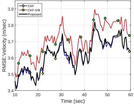
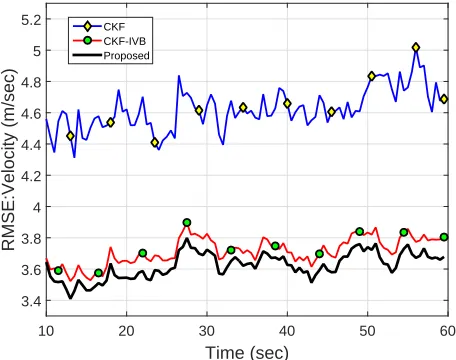
In Figure 1 and 2, we depict the position and velocity RMSE values, respectively, of the three filters when the observation noise is sampled from Gaussian distribution only, i.e., when there are no outliers present. We note that the conventional CKF filter and the proposed filter have almost similar performances in this case; however, the robust CKF-IVB filter suffers performance degradation. It is owing to the reason that a CKF-IVB filter is based on the assumption of t-distributed observation noise and hence in the case of a Gaussian distributed noise, it does not perform as well as a conventional filter. On the other hand, the proposed filter incorporates both the Gaussian as well as t-distributed noise models in a BMA framework and hence performs as good as a conventional CKF. In Figure 3 and 4, we plot the RMSE values of the various filters for outliers contaminated observation noise generated using (44). Note that, owing to the effect of outliers, the CKF filter suffers a large degradation in performance. Whereas the proposed filter as well as the CKF-IVB filter show robust performance in the presence of outliers. Also, the proposed filter is performing better than the CKF-IVB filter even in the presence of outliers. In Table III, we depict the RMSE values averaged over the entire simulation time. We note that in the absence of outliers, the proposed filter shows a 5% improvement in position RMSE over the CKF-IVB filter; whereas, it shows a 38% improvement in position RMSE, over the standard CKF, in the presence of outliers.
Finally, to compare the computational costs of these meth-ods, we run these methods 1000 times under the same con-ditions on MATLAB 2015a using a core-i7 2.6GHZ CPU with 16GB RAM. The average computational times for a single iteration are given in Table IV. Note that the proposed filter is approximately 2.5 times faster than the robust CKF filter based on IVB method; whereas, it takes about twice the computational time as that required by a standard CKF.
2The values of π
ji essentially model the fact that outliers occur only infrequently. We have set πji such that, irrespective of the previous noise sample, the probability that the next noise sample comes from a Gaussian distribution is90%.
TABLE IV
COMPARISON OF AVERAGE COMPUTATIONAL TIME FOR ONE ITERATION OF EACH METHOD
Filter CKF CFK-IVB Proposed
Time (msec) 25 109.2 43.7
Time (sec)
10 20 30 40 50 60
RMSE:Position (m)
12 12.5 13 13.5 14 14.5
CKF CKF-IVB Proposed
Fig. 1. Position RMSE values of CKF, CKF-IVB and the proposed filter, when there are no outliers.
Time (sec)
10 20 30 40 50 60
RMSE:Velocity (m/sec)
3.4 3.5 3.6 3.7 3.8
3.9 CKFCKF-IVB Proposed
Fig. 2. Velocity RMSE values of CKF, CKF-IVB and the proposed filter, when there are no outliers.
IV. CONCLUSIONS
[image:8.612.320.553.356.537.2]Time (sec)
10 20 30 40 50 60
RMSE:Position (m)
12 14 16 18 20 22 24
[image:9.612.63.288.52.234.2]CKF CKF-IVB Proposed
Fig. 3. Position RMSE values of CKF, CKF-IVB and the proposed filter, in the presence of outliers.
Time (sec)
10 20 30 40 50 60
RMSE:Velocity (m/sec)
3.4 3.6 3.8 4 4.2 4.4 4.6 4.8 5
5.2 CKF
CKF-IVB Proposed
Fig. 4. Velocity RMSE values of CKF, CKF-IVB and the proposed filter, in the presence of outliers.
assumption (GA) cubature Kalman filter. In the presence of outliers, the proposed algorithm outperformed both the GA filter as well as the robust IVB filter. Moreover, from the perspective of computational cost, the proposed algorithm was found to be approximately 2.5 times more efficient than the standard IVB based robust solution. Consequently, the proposed filter appears to be an admissible substitute for its traditional counterparts.
ACKNOWLEDGMENT
This work was supported in part by funding from the Higher Education Commission (HEC), Government of Pakistan.
REFERENCES
[1] A. J. Haug,Bayesian estimation and tracking: a practical guide. John Wiley & Sons, 2012.
[2] R. Pich´e, S. S¨arkk¨a, and J. Hartikainen, “Recursive outlier-robust filtering and smoothing for nonlinear systems using the
multivariate student-t distribution,” inProc. from the IEEE Inter-national Workshp on Machine Learning for Signal Processing (MLSP). IEEE, 2012, pp. 1–6.
[3] S. S. Khalid, N. U. Rehman, and S. Abrar, “Robust stochastic integration filtering for nonlinear systems under multivariate t-distributed uncertainties,”Signal Processing, vol. 140, pp. 53– 59, 2017.
[4] M. Roth, E. ¨Ozkan, and F. Gustafsson, “A Student t-filter for heavy tailed process and measurement noise,” in IEEE Intl. Conference on Acoustics, Speech and Signal Processing, 2013, pp. 5770–5774.
[5] Y. Huang, Y. Zhang, N. Li, and J. Chambers, “A robust Gaussian approximate filter for nonlinear systems with heavy tailed measurement noises,” in Proc. from the IEEE Interna-tional Conference on Acoustics, Speech and Signal Processing (ICASSP). IEEE, 2016, pp. 4209–4213.
[6] ——, “A robust Gaussian approximate fixed-interval smoother for nonlinear systems with heavy-tailed process and measure-ment noises,”IEEE Signal Processing Letters, vol. 23, no. 4, pp. 468–472, 2016.
[7] B. Liu, “Robust particle filter by dynamic averaging of multiple noise models,” inProc. from the IEEE International Conference on Acoustics, Speech and Signal Processing (ICASSP). IEEE, 2017, pp. 4034–4038.
[8] Y. Huang and Y. Zhang, “Robust students t-based stochastic cubature filter for nonlinear systems with heavy-tailed process and measurement noises,”IEEE Access, vol. 5, pp. 7964–7974, 2017.
[9] Y. Huang, Y. Zhang, P. Shi, Z. Wu, J. Qian, and J. A. Chambers, “Robust Kalman filters based on Gaussian scale mixture distri-butions with application to target tracking,”IEEE Transactions on Systems, Man, and Cybernetics: Systems, 2017.
[10] A. Kiring, “Tracking in wireless sensor networks with correlated and sparse measurements,” Ph.D. dissertation, Department of Automatic Control and Systems Engineering, The University of Sheffield, Western Bank, Sheffield, S10 2TN, 2017. [11] S. Kotz and S. Nadarajah,Multivariatet-distributions and their
applications. Cambridge University Press, 2004.
[12] I. Arasaratnam, S. Haykin, and R. J. Elliott, “Discrete-time nonlinear filtering algorithms using Gauss–Hermite quadrature,”
Proceedings of the IEEE, vol. 95, no. 5, pp. 953–977, 2007. [13] ´A. F. Garc´ıa-Fern´andez, L. Svensson, M. R. Morelande, and
S. S¨arkk¨a, “Posterior linearization filter: Principles and imple-mentation using sigma points,” IEEE transactions on signal processing, vol. 63, no. 20, pp. 5561–5573, 2015.
[14] S. Challa, Fundamentals of object tracking. Cambridge University Press, 2011.
[15] V. ˇSm´ıdl and A. Quinn,The variational Bayes method in signal processing. Springer Science & Business Media, 2006. [16] G. C. Goodwin and K. S. Sin,Adaptive filtering prediction and
control. Courier Corporation, 2014.
[17] I. Arasaratnam and S. Haykin, “Cubature Kalman filters,”IEEE Transactions on automatic control, vol. 54, no. 6, pp. 1254– 1269, 2009.
[18] Y. Wu, D. Hu, M. Wu, and X. Hu, “A numerical-integration perspective on Gaussian filters,”IEEE Transactions on Signal Processing, vol. 54, no. 8, pp. 2910–2921, 2006.
[19] B. Jia, M. Xin, and Y. Cheng, “High-degree cubature Kalman filter,”Automatica, vol. 49, no. 2, pp. 510–518, 2013. [20] Y. Bar-Shalom, X. R. Li, and T. Kirubarajan,Estimation with
[image:9.612.60.288.273.453.2]