Nonlinear predictive model selection and model averaging using information criteria

This is a repository copy of

Nonlinear predictive model selection and model averaging

using information criteria

.

White Rose Research Online URL for this paper:

http://eprints.whiterose.ac.uk/133030/

Version: Published Version

Article:

Gu, Y., Wei, H. orcid.org/0000-0002-4704-7346 and Balikhin, M. (2018) Nonlinear

predictive model selection and model averaging using information criteria. Systems

Science and Control Engineering, 6 (1). pp. 319-328. ISSN 2164-2583

https://doi.org/10.1080/21642583.2018.1496042

© 2018 The Author(s). Published by Informa UK Limited, trading as Taylor & Francis

Group. This is an Open Access article distributed under the terms of the Creative

Commons Attribution License (http://creativecommons.org/licenses/by/4.0/), which permits

unrestricted use, distribution, and reproduction in any medium, provided the original work

is properly cited.

eprints@whiterose.ac.uk https://eprints.whiterose.ac.uk/ Reuse

This article is distributed under the terms of the Creative Commons Attribution (CC BY) licence. This licence allows you to distribute, remix, tweak, and build upon the work, even commercially, as long as you credit the authors for the original work. More information and the full terms of the licence here:

https://creativecommons.org/licenses/

Takedown

If you consider content in White Rose Research Online to be in breach of UK law, please notify us by

Full Terms & Conditions of access and use can be found at

http://www.tandfonline.com/action/journalInformation?journalCode=tssc20

Systems Science & Control Engineering

An Open Access Journal

ISSN: (Print) 2164-2583 (Online) Journal homepage: http://www.tandfonline.com/loi/tssc20

Nonlinear predictive model selection and model

averaging using information criteria

Yuanlin Gu, Hua-Liang Wei & Michael M. Balikhin

To cite this article: Yuanlin Gu, Hua-Liang Wei & Michael M. Balikhin (2018) Nonlinear predictive

model selection and model averaging using information criteria, Systems Science & Control Engineering, 6:1, 319-328, DOI: 10.1080/21642583.2018.1496042

To link to this article: https://doi.org/10.1080/21642583.2018.1496042

© 2018 The Author(s). Published by Informa UK Limited, trading as Taylor & Francis Group.

Published online: 09 Jul 2018.

Submit your article to this journal

Article views: 61

SYSTEMS SCIENCE & CONTROL ENGINEERING: AN OPEN ACCESS JOURNAL 2018, VOL. 6, NO. 1, 319–328

https://doi.org/10.1080/21642583.2018.1496042

Nonlinear predictive model selection and model averaging using information

criteria

Yuanlin Gu, Hua-Liang Wei and Michael M. Balikhin

Department of Automatic Control and Systems Engineering, University of Sheffield, Sheffield, UK

ABSTRACT

This paper is concerned with the model selection and model averaging problems in system identifi-cation and data-driven modelling for nonlinear systems. Given a set of data, the objective of model selection is to evaluate a series of candidate models and determine which one best presents the data. Three commonly used criteria, namely, Akaike information criterion, Bayesian information criterion and an adjustable prediction error sum of squares (APRESS) are investigated and their performance in model selection and model averaging is evaluated via a number of case studies using both simu-lation and real data. The results show that APRESS produces better models in terms of generalization performance and model complexity.

ARTICLE HISTORY Received 21 February 2018 Accepted 29 June 2018

KEYWORDS Model selection; model averaging; data-driven modelling; system identification; information criterion

1. Introduction

Model selection plays a fundamental role in choosing a best model from a series of candidate models for data-driven modelling and system identification problems. In general, system identification and data-driven modelling consists of several important steps, including data collec-tion, data processing, selection of representation func-tions, model structure selection, model validation and model refinement (Preacher & Merkle,2012; Solares, Wei, & Billings,2017; Söderström & Stoica,1989).

Among various model selection methods, Akaike infor-mation criterion (AIC) and Bayesian inforinfor-mation criterion (BIC) are two most popular measures. Since AIC was firstly proposed in 1974 (Akaike,1974), many variations of AIC have been developed for model selection. For example, the second-order Akaike information criterion (AICc) was developed for small sample size data modelling problems in 1989 (Brockwell & Davis,1991; Hurvich & Tsai,1989); the AIC was designed to approximately estimate the Kullback–Leiber information of models in 1998 (Akaike,

1998); also, the delta AIC and the Akaike weights were introduced to measure how much better the best model is when compared with the other models. In the model selection process, the AIC, delta AIC and AIC weights are calculated for each candidate model. Usually, the ‘best’ model is chosen to be the model with the smallest AIC; the delta AIC calculates the difference between the AIC of each model and the smallest AIC of the ‘best’ model

CONTACT Hua-Liang Wei w.hualiang@sheffield.ac.uk

(Symonds & Moussalli, 2011); the AIC weight is ranged from 0 to 1, which is an analogous to the probability that a candidate model is the best choice (Buckland, Burnham, & Augustin,1997). Drawn on these theories, some model averaging approaches were also developed, for exam-ple, the natural averaging method (Buckland et al.,1997) and full model averaging method (Lukacs, Burnham, & Anderson,2010). Over the past few decades, AIC and its variations have been used to solve a wide range of model selection problems including those in ecology (Johnson & Omland,2004) and phylogenetics (Posada & Buckley,

2004), among others.

Another commonly used model selection criterion is BIC, which was proposed by Schwarz in 1978 (Schwarz,

1978). It is also referred to as the Schwarz information criterion, or the Schwarz BIC. Similar to AIC, BIC is also calculated for each candidate model and the model with the smallest BIC is chosen to be the best model (Kass & Raftery,1995). The only difference between AIC and BIC is that BIC uses a larger penalty on the increment of the model terms. In recent years, BIC has also been increas-ingly used as model selection criterion (Cobos et al.,2014; Hooten & Hobbs,2015; Vrieze, 2012; Watanabe, 2013). Based on the investigation of vast literature on applica-tions and comparative studies of the two criteria (e.g. see Aho, Derryberry, & Peterson,2014; Burnham & Anderson,

2004; Burnham, Anderson, & Huyvaert,2011; Chaurasia & Harel,2013; Claeskens & Hjort,2008; Johnson & Omland,

© 2018 The Author(s). Published by Informa UK Limited, trading as Taylor & Francis Group.

2004; Kuha,2004; Medel & Salgado,2013; Posada & Buck-ley,2004; Vrieze,2012), it can be noted that both AIC and BIC have their own advantages and limitations. It cannot be guaranteed that one is better than another regard-less of application scenarios. The reason is that the data, model type and other aspects of the modelling problems can be significantly important in determining which of the criteria is more suitable.

Both AIC and BIC have been widely applied on model selection problems. However, there still exists large room for improvement. For example, it lacks evidence that the two criteria can also work well for complex nonlin-ear system identification problems. Although AIC and BIC can usually produce good model selection result based on the assumption that the ‘true’ model is among the candidate models, they may fail to select the best model when the system is very complex and neither of the candidate models can sufficiently represent the data. These situations often occur when the model structure or some prior information is unknown. To solve the model selection problem of nonlinear system identification, the cross-validation (CV) based criterion (Stone,1974) and its two variations, the Leave-One-Out (LOO), also called Predicted Residuals Sum of Squares (PRESS) (Allen,1974; Chen, Hong, Harris, & Sharkey,2004; Hong, Sharkey, & Warwick,2003), and generalized cross-validation (GCV) (Golub, Heath, & Wahba, 1979), were developed. Most recently, a modified GCV criterion, also known as adjusted predicted sum of squares (APRESS), was also proposed for nonlinear systems identification (Billings & Wei,2008).

Based on above considerations, it is essential to inves-tigate AIC, BIC and APRESS, to figure out which one works better for model selection of nonlinear system identifica-tion and data-driven modelling problems. In this study, case studies using simulation and real data were car-ried out and the three criteria were used to select a best model from a set of candidate models. The predic-tion performances of the models which are selected by the three criteria were evaluated and compared, to find out which method gives better model selection result. In addition, a model averaging approach is developed based on the full model averaging method to improve the model robustness.

The paper is organized as follows. The nonlinear autoregressive moving average with exogenous input (NARMAX) model and orthogonal forward regression (OFR) algorithm are briefly reviewed in Section2. Section

3introduces the model selection and averaging meth-ods using AIC, BIC and APRESS. In Section4, case studies are given to illustrate the performances of these methods. The paper is concluded in Section5.

2. NARMAX model and OFR algorithm

In this study, the candidate models are chosen to be the NARMAX model structure, which can be described as (Chen & Billings,1989):

y(t)₌F[y(k₋1),. . .,y(k₋ny),u(k−1),. . .,

×u(k₋nu),e(k−1),. . .,e(k−ne)], (1)

wherey(k)andu(k)are systems output and input signals;

e(k)is a noise component with zero mean and finite vari-ance; the noise can be assumed to be white Gaussian in many applications.ny,nuandne are the maximum lags for the system output, input and noise.F[_·] is some non-linear function. A polynomial NARX model can be written as the following linear-in-the-parameters form:

y(k)₌ M

m=1

θmϕm(k)+e(k), (2)

whereϕ_m(k)₌ϕ_m(ϑ (k))are the model terms generated from the regressor vector ϑ (k)₌[y(k₋1),. . .,y(k₋ ny),u(k−1),. . .,u(k−nu)]T,θm are the unknown para-meters andMis the number of candidate model terms.

The NARMAX structure can be identified by an OFR algorithm (Chen, Billings, & Luo,1989), which can be used to select significant model terms according to an error reduction ratio index (ERR), and estimate model param-eters simultaneously (Chen et al., 1989; Wei, Billings, & Liu,2004). The NARMAX model and the OFR algorithm have been successfully applied to solve a wide range of real-world problems in various fields including engi-neering (Zhang, Zhu, & Gu,2017), ecological (Marshall et al.,2016), environmental (Bigg et al.,2014), geophysi-cal (Balikhin et al.,2011; Boynton, Balikhin, Billings, Wei, & Ganushkina,2011), medical (Billings, Wei, Thomas, Lin-nane, & Hope-Gill,2013), and neurophysiological (Li, Wei, Billings, & Sarrigiannis,2016) sciences.

The OFR algorithm is briefly introduced as follows (Chen et al., 1989). Let y₌[y(1),. . .,y(N)]T be a vec-tor of measure outputs at N time instances anϕm=

[ϕm(1),. . .,ϕm(N)]T be the vector formed by the m-th model term(m₌1, 2,. . .,M). LetD_{= {}δj: 1≤j≤M}be

the model term dictionary, the objective of OFR algorithm is to find a subset Dn= {δl1,. . .,δln} so that y can be

explained:

y₌

n

i=1

θliδli+e. (3)

For the full dictionaryD, the ERR index of each candi-date model term can be calculated by:

ERR(1)[i]₌ (r T

0δi)2 (rT₀r0)(δTiδi)

SYSTEMS SCIENCE & CONTROL ENGINEERING: AN OPEN ACCESS JOURNAL 321

wherei₌1, 2,. . .,M. The first selected model term can then be identified as:

l1=arg max 1≤i≤M{ERR

(1)_{[i]}. (5)}

Then the first significant model term of the subset can be selected as ϕ_l1, and the first associated orthogonal variable can be defined asq₁₌δl1. Letr0=y, set:

r12=r02−

(rT₀q₁)2

qT₁q₁ . (6)

After removal ϕ_l1 from D, the dictionary D is then reduced to a sub-dictionaryDM−1, consisting of M−1

model candidates. At steps(s≥2), theM−s+1 bases are first transformed into new group of orthogonalized base [q(₁s),q(₂s),. . .,q(_Ms)_−s+1]with orthogonalization trans-formation.

q(_js)=δj− s−1

r=1

δT_jq_r qT

rqr

q_r, (7)

whereq_r(r₌1, 2,. . .,s₋1)are orthogonal vectors,δj(j= 1, 2,. . .,M₋s₊1) are the basis of unselected model terms of subsetDM−s+1andq_j(s)(j=1, 2,. . .,M−s+1)

are the new orthogonalized bases. The rest of the model terms can then be identified step by step using the ERR index of orthogonalized subsetsDM−s+1:

ERR(s)[j]₌ (y T_q(s)

j )

2

(yT_y)(q(s)T j q

(s)

j )

, (8)

ls=arg max

1≤j≤M−s+1{ERR (1)_[j]

}. (9)

Thes-th significant model term of the subset can be selected asϕls, and thes-th associated orthogonal

vari-able can be defined asq_s=q(_ls) s . Then:

r_s2₌rs−12−

(rT_s−1q_s)2

qT sqs

. (10)

Recursively, the significant model terms of the subset {δl1,. . .,δln}can be identified step by step. By summing

(10) forsfrom 1 ton, yields:

r_n2₌y2₋

n

s=1

(rT s−1qs)

2

qT sqs

. (11)

Ther_n2 is called residual sum of squares, or sum squared error. The mean square error (MSE) of the model can be calculated asr_n2/n, which can be used to form model selection criteria such as AIC, BIC and APRESS.

3. Model selection and model averaging methods for nonlinear modelling

This section introduces model selection and averaging approaches based on AIC, BIC and APRESS.

3.1. Model selection with AIC, BIC and APRESS

AIC and BIC can be calculated as (Akaike,1974; Schwarz,

1978):

AIC(k)_{= −}2 ln(L)₊2k, (12)

BIC(k)_{= −}2 ln(L)₊kln(N), (13)

wherekis the number of fitted parameters in the model,L

is the maximum likelihood estimate for the model andN

is the sample size. As mentioned earlier, for least square based regression analysis, AIC and BIC can be directly calculated by using MSE, as (Hurvich & Tsai,1989):

AIC(k)₌Nln(MSE(k))₊2k, (14)

BIC(k)₌Nln(MSE(k))₊kln(N), (15)

where MSE(k)is the MSE of the candidate model. Equa-tions (14) and (15) are and their variants have been applied for nonlinear and generalized linear model identi-fication (see, for example, Blake & Kapetanios,2003; Egri-oglu, Aladag, & Gunay,2008; Liu, Lin, & Ghosh,2007; Wei, Zhu, Billings, & Balikhin,2007). The APRESS can be easily calculated in each term selection step in OFR algorithm. It is defined as (Billings & Wei,2008; Wei & Billings,2008):

APRESS(k)₌p(k)MSE(k)

=

1 1₋((C(k,α))/N)

2

MSE(k), (16)

wherep(k)is a penalty function defined in terms of the cost function C(k,α)₌k×α with α being an tuning parameter.

Table 1.The advantage and disadvantage of AIC, BIC and APRESS.

Criterion Advantage Limitation

AIC • AIC minimizes useful risk function when true model is not a candidate and the model is complex

• AIC-based model performs not well for out-of-sample data • AIC-based model is often more complicated

BIC • BIC is consistent in selecting true model when model is a candidate • BIC is not consistent when the model is too complex or the uncertainty is too strong

• BIC-based model has better out-of-sample performance APRESS • APRESS is easy to implement in the OFR algorithm for nonlinear

dynamic modelling

• APRESS has a tuning parameter so that it needs a figure to determine the optimal turning point

• APRESS have been applied for nonlinear model selection of many applications

of the system. From the investigation of the literature, a summary of the reported advantages and limitations of the AIC/BIC/APRESS is given in Table1(Aho et al.,2014; Billings & Wei,2008; Hooten & Hobbs,2015; Johnson & Omland,2004; Medel & Salgado,2013; Posada & Buck-ley,2004; Vrieze,2012; Wei & Billings,2008; Wei, Billings, & Balikhin,2006).

3.2. Model averaging with AIC, BIC and APRESS

Model averaging is a widely applied method to deal with model uncertainty and reduce or eliminate the risk of using only a single model. Model averaging approaches such as AIC- and BIC-based averaging methods have been used in many applications (Asatryan & Feld,2015; Cade,

2015; Kontis et al.,2017; Moral-Benito,2015). The model averaging approach with AIC involves the computation of the delta AIC and the Akaike weights. The delta AIC can be calculated as (Symonds & Moussalli,2011):

AICci =AICci−AICcmin, (17)

where AICciis the AIC value for thei-th candidate model,

AICcmin is the minimum AIC of all theMcandidate

mod-els, andi₌1, 2,. . .,M. The Akaike weight indicates the probability that an individual candidate model is the best model. The Akaike weight fori-th candidate mode is com-puted as (Buckland et al.,1997):

ωi=

exp(−0.5AICci)

M

j=1exp(−0.5AICcj)

, (18)

whereω_iis the Akaike weight for thei-th candidate model and i₌1, 2,. . .,M. Then, the averaged parameter esti-mate of ‘full model averaging’ is calculated as follows:

_β¯=M

i=1

ω_iβˆ_i. (19)

To produce averaged model based on BIC and APRESS, a simple approach is to replaced AIC by BIC and APRESS, to calculate the BIC and APRESS weights of model param-eters of all candidate models. The averaged paramparam-eters can then be computed using formula (19). This method is

simple to implement. More importantly, it is easy to deter-mine which of the three criteria gives the best-averaged model. The advantage of the averaged model is that it is, in general, more robust than the single ‘best’ model deter-mined by the model selection criterion. This is because a single model only contains a limit number of model terms suggested by model selection criterion. If a model selec-tion criterion fails to detect the correct number of model terms, the model terms of the single model may be insuf-ficient to well represent the system. On the contrary, the averaged model uses the information of all the candidate models and each candidate model gives its contribution according to their weights based on the model selection criterion. Therefore, when the single model selected by the model selection criterion is not the best, the perfor-mance of the averaged model is usually better than that of the single model. However, it should also be noted that a model with more terms is not necessarily always bet-ter than a model with less bet-terms, because some bet-terms may be redundant and may deteriorate the model pre-diction performance. Therefore, it is not always true that the averaged model is better than a single model, but the averaged model is often more robust in case where there is large uncertainty in the data collection, model structure and model parameter, etc.

4. Case studies

In this section, case studies are carried out to evaluate the performances of the proposed model selection and model averaging methods.

4.1. A simulation example

Consider a nonlinear system described by the model below:

y(t)_{= −}u(t₋1)_|y(t₋1)_{| +}0.5u2(t₋1)

+u2(t₋2)₊y(t₋2)u(t₋1)₊ξ(t), (20)

SYSTEMS SCIENCE & CONTROL ENGINEERING: AN OPEN ACCESS JOURNAL 323

ratio (SNR) of the data is about 10 dB. A total number of 500 input-output data points were generated. The first 250 points were used for model estimation and selection and the second 250 points were used for performance test. A regression vector can be defined as:

ϕ(t)₌[y(t₋1),y(t₋2),u(t₋1),u(t₋2)]T (21)

with the maximum time lags of ny=nu=2. The ini-tial full model was chosen to be a polynomial form with nonlinear degree ofl₌2. The full dictionary contains a total number of 15 model terms:_{y(t₋1),y(t₋2),u(t₋

1),u(t−2),y(t−1)×y(t−1),y(t−1)×y(t−2),

y(t₋1)_×u(t₋1),y(t₋1)_×u(t₋2),y(t₋2)_×

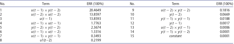
y(t−2),y(t−2)×u(t−1),y(t−2)×u(t−2),u(t−1) ×u(t₋1),u(t₋1)_×u(t₋2),u(t₋2)_×u(t₋2), constant_}. Note that the true model term√_|y(t₋1)_|in (20) is not included in any of the specified candidate model sets. Therefore, all candidate models can only pro-vide an approximation of the true system behaviour, which is accurate to some degree but can never perfectly reconstruct the true system model structure. This is true for most real-world data-driven modelling tasks, where the true system model structure is unknown. The OFR algorithm was used to select model terms from the dictio-nary and estimate the model, and the AIC, BIC and APRESS were used to evaluate all the candidate models. The first 15 model terms are shown in Table2and ranked by the ERR index. It can be seen that the most important terms are selected in the first few steps including the true sys-tem modelu(t₋1)_×y(t₋2). The candidate model is the model with associated number of model terms, for example, the second candidate model is defined to be the model with two terms,u(t−1)×y(t−2)andu(t−2)×

u(t₋2), so on and so forth.

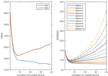
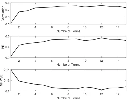
The AIC, BIC and APRESS of all the 15 candidate models were calculated and shown in Figure1and some statisti-cal evaluations of the models suggested by AIC, BIC and APRESS are shown in Table3. The performances of all the candidate models are shown in Figure2. Compared with AIC and BIC, the APRESS suggests a choice of three model terms, which is much smaller than that suggested by AIC and BIC. Also, the model suggested by APRESS, although with fewer number of model terms, possesses slightly

Figure 1.AIC, BIC and APRESS statistics (alpha: adjustable

param-eterα).

better predicative capability. Due to the fact that the pre-diction performances can be affected by the uncertainty brought by the noise, it is normal that any of the models can achieve slightly better statistics of correlation, pre-diction efficiency and error, as long as they include the main components of the true model. However, it is also crucially important to achieve a parsimonious represen-tation for complex nonlinear systems in many application situations, because a model with less variables can largely reduce the work of data collection and benefit the process of understanding the systems. In general, all the three model selection criteria are capable for model selection for this example. It is possibly because that although the model term√_|y(t₋1)_|is not in the candidate term set, it can be approximated using the model termy(t−1)with some polynomial format.

The averaged parameters were calculated based on 15 candidate models using formula (19). Note that all the three averaged models were calculated from the same 15 candidate models and the only difference is that the aver-aged parameter was computed using different weights based on AIC, BIC and APRESS, respectively. A compari-son of the performances of the three averaged models is also shown in Table1. It can be observed that the perfor-mances of the averaged models are slightly better than

Table 2.The first eight terms ranked by the ERR index.

No. Term ERR (100%) No. Term ERR (100%)

1 u(t₋1)_×y(t₋2) 20.4649 9 u(t₋2)_×y(t₋2) 0.1816

2 u(t−2)×u(t−2) 13.8597 10 y(t−2) 0.0669

3 u(t₋1) 13.8593 11 y(t₋1)×y(t₋1) 0.0188

4 u(t₋1)_×u(t₋1) 1.7763 12 y(t₋1) 0.0017

5 y(t−2)×y(t−2) 2.3674 13 u(t−2)×y(t−1) 0.0006

6 u(t₋1)_×u(t₋2) 1.3316 14 y(t₋1)_×y(t₋2) 0.0001

7 u(t−1)×y(t−1) 0.3493 15 constant 0.0001

Table 3.Evaluation of single and averaged models by AIC, BIC and APRESS on train and test datasets.

Correlation coefficient

Normalised root mean square error (NRMSE)

Method Model type

Number of

model terms Training data Test data Training data Test data

AIC Single 6 0.7006 0.6405 0.1109 0.1477

Averaged 15 0.7047 0.6471 0.1102 0.1465

BIC Single 6 0.7006 0.6405 0.1109 0.1477

Averaged 15 0.7004 0.6503 0.1109 0.1461

APRESS Single 3 0.6571 0.6498 0.1172 0.1475

Averaged 15 0.7024 0.6529 0.1109 0.1460

Note: Correlation coefficient is defined to be the correlation between model predictions and corresponding observations.

Figure 2.Performances of all the candidate models on test dataset.

the associated single models, but this is achieved at the price of increasing the model complexity. As mentioned earlier, the true model term √_|y(t₋1)_| in (20) is not included in the specified candidate model terms, as a con-sequence, all the ‘best’ single models suggested by the three criteria just simply achieve a best balance or trade-off between the model representation performance on the test data and the model complexity. For real appli-cations, there would always exist a risk if we only trust a single model to make important decisions or carry out important analyses. The model averaging process, how-ever, is extremely useful to improve the robustness, espe-cially when the true model structure is not included in the specified candidate model set or the model selection method fails to choose the best model.

4.2. A real-world application: Dst index forecast

The magnetosphere can be considered as a complex sys-tem. In order to understand the magnetosphere system, Dst index is often used to measure the magnetic distur-bances (Wei et al.,2006,2007; Wei, Billings, & Balikhin,

2004). In this study, the process of Dst is treated to be an unknown nonlinear system, where the system inputs

Table 4.Dst index and solar wind variables.

Name Description

Dst Dst index

V solar wind speed/velocity (flow speed) [km/s] Bs Southward interplanetary magnetic field p solar wind pressure (flow pressure) [nPa]

VBs V_×Bs/1000;

are solar wind variables and the system output is the Dst index. The description of the inputs and output is given in Table4. All the variables were sampled every 1 hour. It should be noted that VBs is a multiplied input which was suggested to be included in the model inputs (Gonzalez et al.,1994).

The Dst data used in this example is sampled from 1998. There are a total number of 1460 input–output data points. The first half data was used for model estimation and the second half data was used for validation. Similar to the previous discussed simulation example, the OFR algorithm was used to select model terms and estimate the model parameters, and the AIC, BIC and APRESS were used for model selection. The time lag of inputs was cho-sen to be 4 and the nonlinear degree was 2 so that the model is input-alone (Volterra model), meaning that no autoregressive model terms were included in the inputs.

Figure 3.AIC, BIC and APRESS statistics (alpha: adjustable

SYSTEMS SCIENCE & CONTROL ENGINEERING: AN OPEN ACCESS JOURNAL 325

Table 5.Evaluation of single and averaged models by AIC, BIC and APRESS on train and test datasets.

Correlation coefficient NRMSE

Method Model type Number of model terms Training data Test data Training data Test data

AIC Single 38 0.8180 0.5894 0.0657 0.1363

Averaged 40 0.8183 0.6031 0.0657 0.1323

BIC Single 8 0.7868 0.7541 0.0705 0.1046

Averaged 40 0.7886 0.7549 0.0702 0.1047

APRESS Single 7 0.7843 0.6498 0.0709 0.1475

Averaged 40 0.7889 0.7577 0.07702 0.1038

Note: Correlation coefficient is defined to be the correlation between model predictions and corresponding observations.

In total, 40 candidate models were estimated to predict Dst index 1 hour ahead.

The AIC, BIC and APRESS of all the candidate mod-els are shown in Figure3. The number of model terms suggested by AIC, BIC and APRESS are 38, 8 and 7, respec-tively. The evaluation of the prediction performances of the three models are shown in Table5and the perfor-mances of all the 40 estimated models are shown in Figure4. It is clear that AIC fails to select the ‘best’ candi-date model. The model with 38 terms performs poorly in forecasting Dst index 1 hour ahead. On the contrary, the models chosen by BIC and APRESS are quite similar and achieve very similar performances. Comparing the perfor-mances of the two selected models with that produced by all the candidate models, it can be seen that the BIC and APRESS selected nearly the ‘best’ model. Additionally, the model suggested by APRESS involves a relatively smaller number of model terms. Clearly, for this real data exam-ple, both BIC and APRESS are capable for the model selec-tion task. If a parsimonious representaselec-tion is required, the APRESS statistic is superior to the other two model selection criteria.

The averaged parameters were calculated for the can-didate models based on AIC, BIC and APRESS weights. The result of the three averaged models is shown in Table3

and a comparison of predicted and observed Dst index is

Figure 4.Performances of candidate models on test datasets.

Figure 5.Observed and predicted Dst index by averaged models on test dataset.

shown in Figure5. It can be seen that the performances of the averaged models are also similar to the associated single models. Following the discussion above, it can be concluded that the model averaging approaches is con-sistent with the model selection results. The performance of the averaged model is mainly affected by the ‘best’ sin-gle model chosen by AIC, BIC or APRESS, while the other candidate models make smaller contribution to the aver-aged model according to the relevant averaver-aged models.

4.3. A real-world application: estimation of energy performance of residential building

The energy performance of residential building is related to many aspects, for example, surface area, wall area, roof

Table 6.Variable descriptions.

Name Description

y Heating load

x1 Relative compactness

x2 Surface area

x3 Wall area

x4 Roof area

x5 Overall height

x6 Orientation

x7 Glazing area

area, overall height, orientation, glazing area, and glazing area distribution (Tsanas & Xifara,2012). In this example, models are built to represent the relationship between heating load and these factors. The descriptions of these variables (factors) are shown in Table6(Tsanas & Xifara,

2012). There are 768 input–output data points and the first and second half data are used for training and testing, respectively. The nonlinear degree is set to be 3. Similar

Figure 6.AIC, BIC and APRESS statistics (alpha: adjustable

param-eterα).

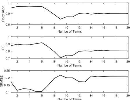
Figure 7.Performance of candidate models on test datasets.

to the process described in Sections 4.1 and 4.2, AIC, BIC and APRESS are used to evaluate a total of 20 candidate models and select the model that can best describe the system.

The plots of AIC, BIC and APRESS of the candidate mod-els are shown in Figure6. Both AIC and BIC suggest the model with 12 model terms. As for APRESS statistics, by setting the adjustable parameterα to be 0, 1,. . . , 10, three apparent turning points are observed at horizon 3, 14 and 17. From Figure7, the model with three terms pro-vides better performances. It can be noted that another advantage of APRESS is that it uses an adjustable param-eterαto calculate the cost function, so that the optimal model length can be determined by the turning points, rather than the smallest value. In this example, if α is set to be any of the single values that is less than 6, it would be difficult to find the optimal point. Thus, the adjustable parameter makes the APRESS more sensible to the optimal solution.

It can be seen from Table7that the averaged model provided by APRESS outperforms those provided by AIC and BIC. This is not surprising, as the single model selected by the APRESS is much better than the models selected by AIC and BIC. Again, it can be conclude that APRESS is supe-rior to AIC and BIC for model selection and model averag-ing for quantifyaverag-ing the energy performance of residential buildings.

5. Conclusion

Investigations have been carried out on model selec-tion and model averaging with three informaselec-tion crite-ria, namely, AIC, BIC and APRESS. Three case studies on system identification and date-driven modelling using both simulation and real datasets are presented, and the associated comparative analysis shows that APRESS is superior to AIC and BIC with several advantages. First, the model produced by APRESS can achieve parsimo-nious representation with good or better prediction per-formance. Second, APRESS is simple to compute incor-porate in the implementation procedure of the OFR algorithm. Third, APRESS is more sensible to the optimal

Table 7.Evaluation of selected and averaged models by AIC, BIC and APRESS on train and test datasets.

Correlation coefficient NRMSE

Method Model type Number of model terms Training data Test data Training data Test data

AIC Single 17 0.9917 0.9024 0.0354 0.2071

Averaged 20 0.9917 0.9022 0.0353 0.2072

BIC Single 17 0.9917 0.9022 0.0354 0.2072

Averaged 20 0.9917 0.9022 0.0354 0.2072

APRESS Single 3 0.9534 0.9639 0.0832 0.1259

Averaged 20 0.9904 0.9120 0.0381 0.1917

SYSTEMS SCIENCE & CONTROL ENGINEERING: AN OPEN ACCESS JOURNAL 327

solution for real data modelling problems. With these benefits, APRESS is recommended for model selection in nonlinear system identification and data-driven mod-elling, especially for real data based modelling problems where the true system model structure is unknown. More-over, a model averaging approach has been introduced and evaluated via the three case studies. The associated results indicate that the averaged model can improve the model robustness and thus it is recommended to use model selection and averaging method together for real data modelling problems of nonlinear systems. The rea-son that APRESS outperforms AIC and BIC in the three case studies is not theoretically justified in the present work. Our future work would include theoretical analysis of the performance of these methods.

Disclosure statement

No potential conflict of interest was reported by the authors.

Funding

This work was supported in part by EU Horizon 2020 Research and Innovation Programme Action Framework under grant agreement 637302, the Engineering and Physical Sciences Research Council (EPSRC) under Grant EP/I011056/1 and EPSRC Platform Grant EP/H00453X/1.

References

Aho, K., Derryberry, D., & Peterson, T. (2014). Model selec-tion for ecologists: The worldviews of AIC and BIC.Ecology. doi.org/10.1890/13-1452.1

Akaike, H. (1974). A new look at the statistical model identifica-tion.IEEE Transactions on Automatic Control,19(6), 716–723. doi:10.1109/TAC.1974.1100705

Akaike, H. (1998). Information theory and an extension of the maximum likelihood principle BT - selected papers of Hiro-tugu Akaike. InSecond international symposium on informa-tion theory(pp. 199–213).doi:10.1007/978-1-4612-1694-0_15 Allen, D. (1974). The relationship between variable selection and data agumentation and a method for prediction. Technomet-rics. Retrieved from http://www.jstor.org/stable/1267500/ npapers2://publication/uuid/A720A675-33B6-4965-91B6-8AAF755AC01C

Asatryan, Z., & Feld, L. P. (2015). Revisiting the link between growth and federalism: A Bayesian model averaging approach. Journal of Comparative Economics,43(3), 772–781.doi:10.1016/ j.jce.2014.04.005

Balikhin, M. A., Boynton, R. J., Walker, S. N., Borovsky, J. E., Billings, S. A., & Wei, H. L. (2011). Using the NARMAX approach to model the evolution of energetic electrons fluxes at geostationary orbit.Geophysical Research Letters, 38(18).doi:10.1029/2011GL048980

Bigg, G. R., Wei, H. L., Wilton, D. J., Zhao, Y., Billings, S. A., Hanna, E., & Kadirkamanathan, V. (2014). A century of variation in the dependence of Greenland iceberg calving on ice sheet sur-face mass balance and regional climate change.Proceedings

of the Royal Society A: Mathematical, Physical and Engineering Sciences,470(2166).doi:10.1098/rspa.2013.0662

Billings, S. A., & Wei, H. L. (2008). An adaptive orthogonal search algorithm for model subset selection and non-linear system identification.International Journal of Control,81(5), 714–724. doi:10.1080/00207170701216311

Billings, C. G., Wei, H. L., Thomas, P., Linnane, S. J., & Hope-Gill, B. D. M. (2013). The prediction of in-flight hypoxaemia using non-linear equations.Respiratory Medicine,107(6), 841–847. doi:10.1016/j.rmed.2013.02.016

Blake, A. P., & Kapetanios, G. (2003). A radial basis func-tion artificial neural network test for neglected nonlin-earity. Econometrics Journal,6(2), 357–373. Retrieved from http://www.jstor.org/stable/23116018

Boynton, R. J., Balikhin, M. A., Billings, S. A., Wei, H. L., & Ganushk-ina, N. (2011). Using the NARMAX OLS-ERR algorithm to obtain the most influential coupling functions that affect the evolution of the magnetosphere.Journal of Geophysical Research: Space Physics,116(5).doi:10.1029/2010JA015505 Brockwell, P. J., & Davis, R. A. (1991). Time series: Theory and

methods.Technometrics,31.doi:10.1007/978-1-4419-0320-4 Buckland, S. T., Burnham, K. P., & Augustin, N. H. (1997). Model

selection: An integral part of inference.Biometrics,53(2), 603. doi:10.2307/2533961

Burnham, K. P., & Anderson, D. R. (2004). Multimodel inference: Understanding AIC and BIC in model selection. Sociologi-cal Methods & Research,33, 261–304.doi:10.1177/004912410 4268644

Burnham, K. P., Anderson, D. R., & Huyvaert, K. P. (2011). AIC model selection and multimodel inference in behav-ioral ecology: Some background, observations, and com-parisons.Behavioral Ecology and Sociobiology,65(1), 23–35. doi:10.1007/s00265-010-1029-6

Cade, B. S. (2015). Model averaging and muddled multi-model inferences.Ecology,96(9), 2370–2382. doi:10.1890/14-1639.1

Chaurasia, A., & Harel, O. (2013). Model selection rates of information based criteria.Electronic Journal of Statistics,7, 2762–2793.doi:10.1214/13-EJS861

Chen, S., & Billings, S. A. (1989). Representations of non-linear systems: The NARMAX model.International Journal of Control, 49(3), 1013–1032.doi:10.1080/00207178908559683 Chen, S., Billings, S. A., & Luo, W. (1989). Orthogonal least squares

methods and their application to non-linear system iden-tification.International Journal of Control,50(5), 1873–1896. doi:10.1080/00207178908953472

Chen, S., Hong, X., Harris, C. J., & Sharkey, P. M. (2004). Sparse modeling using orthogonal forward regression with PRESS statistic and regularization. IEEE Transactions on Systems, Man and Cybernetics, Part B (Cybernetics), 34(2), 898–911. doi:10.1109/TSMCB.2003.817107

Claeskens, G., & Hjort, N. (2008).Model selection and model aver-aging. Cambridge: Cambridge University Press.

Cobos, C., Munoz-Collazos, H., Urbano-Munoz, R., Mendoza, M., Leon, E., & Herrera-Viedma, E. (2014). Clustering of web search results based on the cuckoo search algorithm and bal-anced Bayesian information criterion.Information Sciences, 281, 248–264.doi:10.1016/j.ins.2014.05.047

Golub, G. H., Heath, M., & Wahba, G. (1979). Generalized cross-validation as a method for choosing a good ridge parameter. Technometrics,21(2), 215–223.doi:10.1080/00401706.1979. 10489751

Gonzalez, W. D., Joselyn, J. A., Kamide, Y., Kroehl, H. W., Ros-toker, G., Tsurutani, B. T., & Vasyliunas, V. M. (1994). What is a geomagnetic storm? Journal of Geophysical Research. doi:10.1029/93ja02867

Hong, X., Sharkey, P. M., & Warwick, K. (2003). A robust non-linear identification algorithm using PRESS statistic and forward regression. IEEE Transactions on Neural Networks. doi:10.1109/TNN.2003.809422

Hooten, M. B., & Hobbs, N. T. (2015). A guide to Bayesian model selection for ecologists.Ecological Monographs,85(1), 3–28. doi:10.1890/14-0661.1

Hurvich, C. M., & Tsai, C. L. (1989). Regression and time series model selection in small samples.Biometrika,76(2), 297–307. doi:10.2307/2336663

Johnson, J. B., & Omland, K. S. (2004). Model selection in ecology and evolution. Trends in Ecology and Evolution. doi:10.1016/j.tree.2003.10.013

Kass, R., & Raftery, A. (1995). Bayes factors. Journal of the American Statistical Association, 90, 773–795. doi:10.1080/ 01621459.1995.10476572

Kontis, V., Bennett, J. E., Mathers, C. D., Li, G., Foreman, K., & Ezzati, M. (2017). Future life expectancy in 35 industrialised coun-tries: Projections with a Bayesian model ensemble.The Lancet, 389(10076), 1323–1335.doi:10.1016/S0140-6736(16)32381-9 Kuha, J. (2004). AIC and BIC: Comparisons of assumptions and performance. Sociological Methods & Research, 33(2), 188–229.doi:10.1177/0049124103262065

Li, Y., Wei, H.-L., Billings, S. A., & Sarrigiannis, P. G. (2016). Identification of nonlinear time-varying systems using an online sliding-window and common model structure selec-tion (CMSS) approach with applicaselec-tions to EEG.International Journal of Systems Science,47(11), 2671–2681.doi:10.1080/ 00207721.2015.1014448

Liu, D., Lin, X., & Ghosh, D. (2007). Semiparametric regression of multidimensional genetic pathway data: Least-squares kernel machines and linear mixed models.Biometrics, 63, 1079–1088.doi:10.1111/j.1541-0420.2007.00799.x

Lukacs, P. M., Burnham, K. P., & Anderson, D. R. (2010). Model selection bias and Freedman’s paradox.Annals of the Insti-tute of Statistical Mathematics,62(1), 117–125.doi:10.1007/ s10463-009-0234-4

Marshall, A. M., Bigg, G. R., van Leeuwen, S. M., Pinnegar, J. K., Wei, H. L., Webb, T. J., & Blanchard, J. L. (2016). Quantifying heterogeneous responses of fish community size structure using novel combined statistical techniques.Global Change Biology,22(5), 1755–1768.doi:10.1111/gcb.13190

Medel, C. A., & Salgado, S. C. (2013). Does the BIC estimate and forecast better than the AIC?Revista de Analisis Economico, 28(1), 47–64.doi:10.4067/S0718-88702013000100003 Moral-Benito, E. (2015). Model averaging in economics: An

overview.Journal of Economic Surveys,29(1), 46–75.doi:10. 1111/joes.12044

Posada, D., & Buckley, T. R. (2004). Model selection and model averaging in phylogenetics: Advantages of Akaike

information criterion and Bayesian approaches over likeli-hood ratio tests.Systematic Biology.doi:10.1080/1063515049 0522304

Preacher, K. J., & Merkle, E. C. (2012). The problem of model selection uncertainty in structural equation modeling. Psy-chological Methods,17(1), 1–14.doi:10.1037/a0026804 Schwarz, G. (1978). Estimating the dimension of a model.The

Annals of Statistics,6(2), 461–464.doi:10.1214/aos/1176344136 Söderström, T., & Stoica, P. (1989).System identification. London:

Prentice Hall Int.

Solares, J. R. A., Wei, H. L., & Billings, S. A. (2017). A novel logistic-NARX model as a classifier for dynamic binary classifi-cation.Neural Computing and Applications, 1–15.doi:10.1007/ s00521-017-2976-x

Stone, M. (1974). Cross-Validatory choice and assessment of statistical predictions.Journal of the Royal Statistical Society, 36(2), 111–147.doi:10.2307/2984809

Symonds, M. R. E., & Moussalli, A. (2011). A brief guide to model selection, multimodel inference and model averaging in behavioural ecology using Akaike’s information criterion. Behavioral Ecology and Sociobiology. doi:10.1007/s00265-010-1037-6

Tsanas, A., & Xifara, A. (2012). Accurate quantitative estimation of energy performance of residential buildings using statisti-cal machine learning tools.Energy and Buildings,49, 560–567. doi:10.1016/j.enbuild.2012.03.003

Vrieze, S. I. (2012). Model selection and psychological theory: A discussion of the differences between the Akaike information criterion (AIC) and the Bayesian information criterion (BIC). Psychological Methods,17, 228–243.doi:10.1037/a0027127 Watanabe, S. (2013). A widely applicable Bayesian information

criterion.Journal of Machine Learning Research,14, 867–897. Wei, H. L., & Billings, S. A. (2008). Model structure selection

using an integrated forward orthogonal search algorithm assisted by squared correlation and mutual information. International Journal of Modelling, Identification and Control, 3(4), 341.doi:10.1504/IJMIC.2008.020543

Wei, H. L., Billings, S. A., & Balikhin, M. A. (2006). Wavelet based non-parametric NARX models for nonlinear input-output sys-tem identification.International Journal of Systems Science, 37(15), 1089–1096.doi:10.1080/00207720600903011 Wei, H. L., Billings, S. A., & Balikhin, M. (2004). Prediction of

the Dst index using multiresolution wavelet models.Journal of Geophysical Research: Space Physics,109(A7).doi:10.1029/ 2003JA010332

Wei, H. L., Billings, S. A., & Liu, J. (2004). Term and variable selec-tion for non-linear system identificaselec-tion.International Jour-nal of Control,77(1), 86–110.doi:10.1080/002071703100016 39640

Wei, H. L., Zhu, D. Q., Billings, S. A., & Balikhin, M. A. (2007). Forecasting the geomagnetic activity of the Dst index using multiscale radial basis function networks. Advances in Space Research,40(12), 1863–1870.doi:10.1016/j.asr.2007. 02.080