Harp: Collective Communication on Hadoop

Harp: Collective Communication on Hadoop

Bingjing Zhang, Yang Ruan, Judy Qiu Computer Science Department

Indiana University Bloomington, IN, USA

Abstract—Big data tools have evolved rapidly in recent years.

MapReduce is very successful but not optimized for many important analytics; especially those involving iteration. In this regard, Iterative MapReduce frameworks improve performance of MapReduce job chains through caching. Further Pregel, Giraph and GraphLab abstract data as a graph and process it in iterations. However, all these tools are designed with fixed data abstraction and have limitations in communication support. In this paper, we introduce a collective communication layer which provides optimized communication operations on several important data abstractions such as arrays, key-values and graphs, and define a Map-Collective model which serves the diverse communication demands in different parallel applications. In addition, we design our enhancements as plug-ins to Hadoop so they can be used with the rich Apache Big Data Stack. Then for example, Hadoop can do in-memory communication between Map tasks without writing intermediate data to HDFS. With improved expressiveness and excellent performance on collective communication, we can simultaneously support various applications from HPC to Cloud systems together with a high performance Apache Big Data Stack.

Keywords—Collective Communication; Big Data Processing; Hadoop

I. INTRODUCTION

It is estimated that organizations with high-end computing infrastructures and data centers are doubling the amount of data they archive every year. Sophisticated machine learning techniques aim to offer the best results to return to the user. It did not take long for these ideas to be applied to the full range of scientific challenges. Many of the primary software tools used to do large-scale data analysis are required by these applications to optimize their performance. There is a need to integrate features of traditional high-performance computing, such as scientific libraries, communication and resource management middleware, with the rich set of capabilities found in the commercial Big Data ecosystem such as Apache open source software stack. The overarching question we will address is “How should we design, analyze and implement a unified and interoperable infrastructure to meet the requirements of a broad set of data intensive applications?”

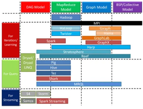
The primary software tools used to do the large-scale data analysis has evolved rapidly as shown in Fig. 1. The last decade witnessed a huge computing shift derived from publication of the Google MapReduce paper [1]. Since then, its open source version Hadoop [2] has become the mainstream of big data processing, with many other tools emerging to process different big data problems, extending the original MapReduce model to include iterative MapReduce. Tools such as Twister [3] and HaLoop [4] can cache loop invariant data locally to avoid repeat input data loading in a MapReduce job chain.

Spark [5] also uses caching to accelerate iterative algorithms without restricting computation to a chain of MapReduce jobs. To process graph data, Google announced Pregel [6] and soon open source versions Giraph [7] and Hama [8] emerged.

Whatever their differences, all such programs are based on a kind of “top-down” design. The whole programming model, from data abstraction to computation and communication pattern, is fixed. Users have to put their applications into the model, which could cause performance inefficiency. For example, in K-Means clustering [9] (Lloyd's algorithm [10]), every successive task needs all the centroids generated in the last iteration. Mahout [11] on Hadoop chooses to reduce the results of all the map tasks in one reduce task and store it on HDFS. This data is then read by all the map tasks in the job at the next iteration. The “reduce” stage can be parallelized by chunking intermediate data to partitions and using multiple reduce tasks to compute each part in parallel. This type of “(multi-)reduce-gather-broadcast” strategy is also applied in other frameworks through in-memory communication, e.g. Twister and Spark.

Regardless, “gather-broadcast” is not an efficient way to relocate the new centroids generated by reduce tasks, especially when the centroids data grows large in size. The time complexity of “gather” is at least kdβ where k is the number of centroids, d is the number of dimensions and β is the communication time used to send each element in the centroids (communication initiation time α is neglected). Also the time complexity of “broadcast” is at least kdβ [12] [13]. Thus the

time complexity of “gather-broadcast” is about 2kdβ. But if we use allgather bucket algorithm [14], it is reduced to kdβ.

In iterative algorithms, communication participated in by all the workers happens once or more per iteration. This makes communication algorithm performance crucial to the efficiency of the whole application. We call this “Collective Communication”. Rather than fixing communication patterns, we decided to separate this layer out and provide collective communication abstraction. Collective communication features in MPI [15], designed for HPC systems and supercomputers. While well defined, there are many limitations. It cannot support high level data abstractions other than arrays, objects, and related communication patterns on them, e.g. shuffling on key-values or message passing along edges in graphs. Another drawback is that it forces users to focus on every detail of a communication call. For example, users have to calculate the buffer size for data receiving, which is difficult to obtain in many applications as the amount of sending data may be very dynamic and unknown to the receivers.

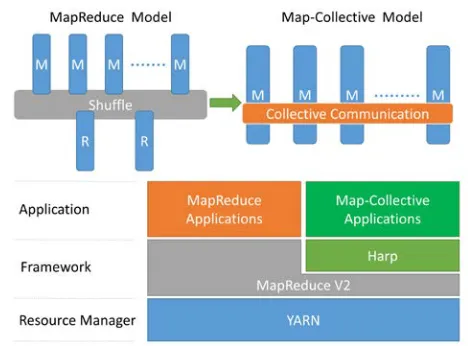
In response to these issues, we present Harp library. Harp provides data abstractions and related communication abstractions with optimized implementation. By plugging Harp into Hadoop, we convert MapReduce model to Map-Collective model and enable efficient in-memory communication between map tasks across a variety of important data analysis applications. The word “harp” symbolizes how parallel processes cooperate through collective communication for efficient data processing, just as strings in harps can make concordant sound (see Fig. 2). The inclusion of collective communication abstraction and Map-Collective model means Harp is neither a replication of MPI nor an attempt to transplant MPI into the Hadoop system [16], as we will elaborate in subsequent sections.

In the rest of this paper, Section 2 discusses about related work. Section 3 describes the abstraction of collective communication. Section 4 shows how Map-Collective model works in Hadoop-Harp. Section 5 gives several applications implemented in Harp. Section 6 shows the performance of Harp through benchmarking on the applications.

II. RELATED WORK

The landscape of big data tools grows bigger and more complicated. Each tool has its own computation model with related data abstraction and communication abstraction in order to achieve optimization for different applications. Before the MapReduce model, MPI was the main tool used for large-scale simulation, exclusive on expensive hardware such as HPC or supercomputers. But MapReduce tries to use commodity machines to solve big data problems. This model defines data abstraction as key-value pairs and computation flow as “map, shuffle and then reduce”. One advantage of this tool is that it doesn’t rely on memory to load and process all the data, instead using local disks. MapReduce model can solve problems where the data size is too large to fit into the memory. Furthermore, it also provides fault tolerance, which is important to big data processing. The open source implementation Hadoop [2] is widely used nowadays in both industry and academia.

MapReduce became popular for its simplicity and scalability, yet is still slow when running iterative algorithms. The resultant chain of MapReduce jobs means repeat input data loading occurs in each iteration. Several frameworks such as Twister [3], HaLoop [4] and Spark [5] solve this problem by caching intermediate data. Another model used for iterative computation is the Graph model, which abstracts data as vertices and edges. Here computation happens on vertices, and each worker caches vertices and related out-edges as graph partitions. The whole parallelization is BSP (Bulk Synchronous Parallel) style. There are two open source projects following Pregel’s design. One is Giraph [7] and another is Hama [8]. Giraph exactly follows iterative BSP graph computation pattern while Hama tries to build a general BSP computation model. By contrast, GraphLab [17] [18] abstracts data as a “data graph” and uses consistency models to control vertex value update. GraphLab was later enhanced with PowerGraph [19] abstraction to reduce the communication overhead. This was also learned by GraphX [20].

The third model is DAG, which abstracts computation flow as a directed acyclic graph. Each vertex in the graph is a process, and each edge is a communication channel between two processes. DAG model is helpful to those applications which have complicated parallel workflows. Dryad [21] is an example of a parallel engine using DAG. Tools employing this model are often used for query and stream data processing.

Some attempts have been made to blend select features of these models. For example, Spark’s RDD data abstraction and transformation operations are very similar to MapReduce model. But it organizes computation tasks as DAGs. Stratosphere [22] and REEF [23] also try to support several different models in one framework. “Broadcast” operation from MPI is added in Hadoop by using distributed cache through a simple algorithm (one-by-one sending). And it is optimized by using BitTorrent technology in Spark [24] or using a pipeline-based chain algorithm in Twister [12] [13].

necessary to build a separated communication layer abstraction. With this we can build a computation model that provides a rich set of communication operations and grants users flexibility in choosing operations suitable to their applications.

A common question is why we don’t use MPI directly since it already offers collective communication abstraction. There are many reasons. Firstly the collective communication in MPI is still limited in abstraction. It provides a low level data abstraction on arrays and objects so that many collective communication operations used in other big data tools are not provided directly in MPI. Besides, MPI doesn’t provide computation abstraction, such that writing MPI applications is difficult compared with other big data tools. Thirdly, MPI is commonly deployed on HPC or supercomputers. Despite projects like [16], it is not as well integrated with cloud environments as Hadoop ecosystems.

III. COLLECTIVE COMMUNICATION ABSTRACTION We have taken several steps to achieve high efficiency. To support different types of communication patterns in big data tools, we abstract data types in a hierarchy. Then we define collective communication operations on top of the data abstractions. Lastly to improve the efficiency of communication, we add memory a management module in implementation for data caching and reuse.

A. Hierarchical Data Abstraction

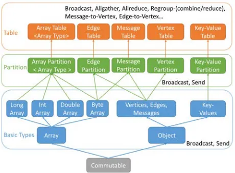
In Fig. 3, we abstract data horizontally as arrays, key-values or vertices, edges and messages in graphs. Vertically we build abstractions from basic types to partitions and tables.

Firstly, any data which can be sent or received is an implementation of interface Commutable. At the lowest level, there are two basic types under this interface: arrays and objects. Based on the component type of an array, currently we have byte array, int array, long array and double array. For object type, to describe graph data there is vertex object, edge object and message object; to describe key-value pairs, we use key object and value object.

Next, at the middle level, basic types are wrapped as array partitions, key-value partitions and graph partitions (edge partition, vertex partition and message partition). Notice that we follow the design of Giraph; edge partition and message partition are built from byte arrays but not from edge objects or message objects directly. When reading, bytes are converted to an edge object or a message object. When writing, either the edge object or the message object is serialized and written back to byte arrays.

At the top level are tables containing several partitions each with a unique partition ID. If two partitions with the same ID are added to the table it will solve the ID conflict by either combining or merging them into one. Tables on different workers are associated with each other through table IDs. Tables sharing the same table ID are considered as one dataset and “collective communication” is defined as redistribution or consolidation of partitions in this dataset. For example, in Fig. 4, a set of tables associated with ID 0 is defined on workers from 0 to N. Partitions from 0 to M are distributed among these tables. A collective communication operation on Table 0 is to move the partitions between these tables. We will talk more in detail about the behavior of partition movement in collective communication operations.

B. Collective Communication Operations

Collective communication operations are defined on top of the data abstractions. Currently three categories of collective communication operations are supported:

1) Collective communication inherited from MPI collective communication operations, such as “broadcast”, “allgather”, and “allreduce”.

2)Collective communication inherited from MapReduce “shuffle-reduce” operation, e.g. “regroup” operation with “combine or reduce” support.

3)Collective communications abstracted from graph communication, such as “regroup vertices or edges”, “move edges to vertices” and “send messages to vertices”.

Some collective communication operations tie to certain data abstractions. For example, graph collective communication operations have to be done on graph data. But for other operations, the boundary is blurred. “allgather” operation can be used on array tables, key-value tables, and vertex tables. But currently we only implement it on array tables and vertex tables. The following is a table which summarizes all the operations identified from applications and related data abstractions (see Table I). We will continue adding other collective communication operations not shown on this table in the future.

If we take another look at Fig. 4 and use “regroup” as an example, for N + 1 workers, workers are ranked from 0 to N. Here Worker 0 is selected as the master worker which collects the partition distribution information on all others. Each worker reports the current table ID and the partition IDs it owns. Table ID is used to identify if the collective communication is on the same dataset. Once all the partition IDs are received, the master worker decides the destination worker IDs of each partition. Usually the decision is done through modulo operation. Once the master’s decision is made, the result is broadcasted to all Fig. 3. Hierarchical Data Abstraction and Collective Communication

workers, after which each worker starts to send out and receive partitions from one another (see Fig. 5).

Each collective communication can be implemented in many different algorithms. For example, we have two implementations of “allreduce”. One is “bidirectional-exchange algorithm” [14] and another is “regroup-allgather algorithm”. When the data size is large and each table has many partitions, “regroup-allgather” is more suitable because it has less data sending and more balanced workload on each worker. But if the table on each worker only has one or a few partitions, “bidirectional-exchange” is more effective. Currently different algorithms are provided in different operation calls, but we intend to provide automatic algorithm selection in the future.

In addition, we also optimize the “decision making” stages of several collective communication operations when the partition distribution is known in the application context. Normally just like in Fig. 5, the master worker has to collect the partition distribution on each worker and broadcast the “regroup” decision to let them know which partition to send and which to receive. But when the partition distribution is known, this step can be skipped. In general, we enrich Harp collective communication library by providing different implementations for each operation so that users can choose the proper one based on the application requirement.

C. Implementation

To make the collective communication abstraction work, we design and implement several components on each worker to send and receive data. These components are resource pool, receiver and data queue. Resource pool is crucial in computation and collective communication of iterative algorithms. In these algorithms, the collective communication operations are called repeatedly and the intermediate data between iterations is similar in size, just with different content. Resource pool caches the data used in the last iteration to enable it to reuse them in the next. Therefore the application can avoid repeat allocation of memory and lower the time used on garbage collection.

The process of sending proceeds as follows: the worker first serializes the data to a byte array fetched from the resource pool and then sends it through the socket. Receiving is managed by the receiver component. It starts a thread to listen to the socket requests. For each request, the receiver spawns a

handler thread to process it. We use “producer-consumer” model to process the data received. For efficiency, data is identified by its related metadata information. Handler threads add the data received to the data queue. The main thread of the worker fetches data from the queue and examines if it belongs to this round of communication. If yes, the data is removed from the queue; otherwise it will be put back into the queue again.

IV. MAP-COLLECTIVE MODEL

The collective communication abstraction we proposed is designed to run in a general environment with a set of parallel Java processes. Each worker only needs a list of all workers’ locations to start the communication. Therefore this work can be used to improve collective communication operations in any existing big data tool. But since communication is hidden in these tools, the applications still cannot benefit from the expressiveness of collective communication abstraction. As a solution we deploy Map-Collective model to enable using collective communications in map tasks. In this section, we are going to talk about several features of Map-Collective model.

A. Hadoop Plugin and Harp Installation

Harp is designed as a plugin to Hadoop. Currently it supports Hadoop-1.2.1 and Hadoop-2.2.0. To install Harp

Fig. 4. Abstraction of Tables and Partitions

Fig. 5. The Process of Regrouping Array Tables TABLE I. Collective Communication Operations and the Data

Abstractions Supported (“√” means “supported” and “implemented” and “○” means “supported” but “not implemented)

Operation Name Array Table

Key-Value Table

Graph Table

Broadcast √ ○ √ (Vertex)

Allgather √ ○ √ (Vertex)

Allreduce √ ○ ○ (Vertex)

Regroup √ √ √ (Edge)

Send all messages to

vertices √

Send all edges to

library, users only need to put the Harp jar package into the Hadoop library directory. For Hadoop 1, users need to configure the job scheduler to the scheduler designed for Map-collective jobs. But in Hadoop 2.0, since YARN resource management layer and MapReduce framework are separated, users are not required to change the scheduler. Instead, they just need to set "mapreduce.framework.name" to "map-collective" in client job configuration. Harp will launch a specialized application master to request resources and schedule Map tasks.

B. MAP-COLLECTIVE INTERFACE

In Map-Collective model, user-defined mapper classes are extended from the class CollectiveMapper which is extended from the class Mapper in the original MapReduce framework. In CollectiveMapper, users need to override a method “mapCollective” with application code. While similar to “mapCollective” method differs from Class Mapper in that it employs KeyValReader to provide flexibility to users; therefore they can either read all key-values into the memory and cache them or read them part by part to fit the memory constraint (see Table II).

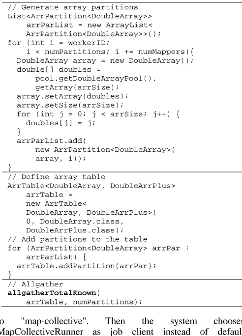
Here is an example of how to do “allgather” in “mapCollective” method (see TABLE III). Firstly we generate several array partitions with arrays fetched from the resource pool and add these partitions into an array list. The total number of partitions on all the workers is specified by numPartitions. Each worker has numPartition/numMappers partition (we assume numPartitions % numMappers = 0). Then we add these partitions in an array table and invoke “allgather”. DoubleArrPlus is the combiner class used in these array tables to solve partition ID conflict in partition receiving. The “allgather” method used here is called “allgatherTotalKnown”. Because the total number of partitions is provided as a parameter in this version of “allgather”, workers don’t need to negotiate the number of partitions to receive from each worker, but send out all the partitions they own to their neighbor directly with the bucket algorithm.

C. BSP Style Parallelism

To enable in-memory collective communication between workers, we need to make every worker alive simultaneously. As a result, instead of dynamic scheduling, we use static scheduling. Workers are separated into different nodes and do collective communication iteratively. The whole parallelism follows the BSP pattern.

Here we use our Harp implementation in Hadoop-2.2.0 to talk about the scheduling mechanism and initialization of the environment. The whole process is similar launching MapReduce applications in Hadoop-2.2.0. In job configuration at client side, users need to set "mapreduce.framework.name"

to "map-collective". Then the system chooses MapCollectiveRunner as job client instead of default YARNRunner for MapReduce jobs. MapCollectiveRunner launches MapCollectiveAppMaster to the cluster. When MapCollectiveAppMaster requests resources, it schedules the tasks to different nodes. This can maximize memory sharing and multi-threading on each node and save the intermediate data size in collective communication.

In the launching stage, MapCollectiveAppMaster records the location of each task and generates two lists. One contains the locations of all the workers and another contains the mapping between map task IDs and worker IDs. These files currently are stored on HDFS and shared among all the workers. To ensure every worker has started, we use a “handshake”-like mechanism to synchronize them. In the first step, the master worker tries to ping its subordinates by sending a message. In the second step, slave workers who received the ping message will send a response back to acknowledge they are alive. In the third step, once the master gets all the responses, it broadcasts a small message to all workers to notify them of the initialization’s success.

When the initialization is done, each worker invokes “mapCollective” method to do computation and communication. We design the interface “doTasks” to enable users to launch multithread tasks. Given an input partition list and a Task object with user-defined “run” method, the “doTasks” method can automatically do multi-threading parallelization and return the outputs.

TABLE II. “mapCollective” interface

protected void mapCollective(

KeyValReader reader,

Context context) throws IOException, InterruptedException {

// Put user code here… }

TABLE III. “Allgather” code example

// Generate array partitions List<ArrPartition<DoubleArray>>

arrParList = new ArrayList< ArrPartition<DoubleArray>>(); for (int i = workerID;

i < numPartitions; i += numMappers){ DoubleArray array = new DoubleArray(); double[] doubles =

pool.getDoubleArrayPool(). getArray(arrSize);

array.setArray(doubles); array.setSize(arrSize);

for (int j = 0; j < arrSize; j++) { doubles[j] = j;

}

arrParList.add(

new ArrPartition<DoubleArray>( array, i));

}

// Define array table

ArrTable<DoubleArray, DoubleArrPlus> arrTable =

new ArrTable<

DoubleArray, DoubleArrPlus>( 0, DoubleArray.class, DoubleArrPlus.class); // Add partitions to the table

for (ArrPartition<DoubleArray> arrPar : arrParList) {

arrTable.addPartition(arrPar); }

// Allgather

allgatherTotalKnown(

D. Fault Tolerance

When it comes to fault tolerance, detection and recovery are crucial system features. Currently our effort is to ensure every worker can report exceptions or faults correctly without getting hung up. With careful implementation and based on the results of testing, this issue is solved.

Fault recovery poses a challenge because the execution flow in each worker is very flexible. Currently we do job level fault recovery. Based on the execution time length of scale, jobs with a large number of iterations can be separated into a small number of jobs, each of which contains several iterations. This naturally forms checkpointing between iterations. Because Map-Collective jobs are very efficient on performance, this method is feasible without generating large overhead. At the same time, we are also investigating task-level recovery by re-synchronizing new launched tasks with other old live tasks.

E. Layered Architecture

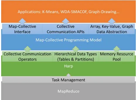
Fig. 6 shows how different layers interface with each other in the Map-collective model. At the bottom level is the MapReduce framework. The modified MapReduce framework exposes the network location of tasks in the cluster to Harp in the upper level. Harp builds collective communication abstraction and provides collective communication operators, hierarchical data types of tables and partitions, and the memory allocation management pool. All these 3 components interface with the Map-Collective programming model. After wrapping, Map-Collective model provides 3 components to the applications: a method interface called mapCollective, a set of collective communication APIs which can be invoked in the mapCollective interface, and the data abstraction of array data, Key-Value data and graph data.

V. APPLICATIONS

We've implemented three applications using Harp: K-Means clustering, Force-directed Graph Drawing Algorithm, and Weighted Deterministic Annealing SMACOF. The first two algorithms are very simple. Both of them use a single collective communication operation per iteration. But the third is much more complicated. It has nested iterations, and two different collective communication operations are used

alternately. In data abstraction, the first and third algorithms use array abstraction, while the second one utilizes graph abstraction. For key-value abstraction, we only implemented Word Count. We don’t introduce it here because it is very simple, with only one “regroup” operation and no iterations.

A. K-Means Clustering

K-Means Clustering is an algorithm to cluster large numbers of data points to a predefined set of clusters. We use Lloyd's algorithm [10] to implement K-Means Clustering in Map-Collective model.

In Hadoop-Harp, each worker loads a part of the data points and caches them into memory as array partitions. The master worker loads the initial centroids file and broadcasts it to all the workers. Later, for every iteration a worker calculates its own local centroids and then uses “allreduce” operation at the end to produce the global centroids of this iteration on each worker. After several iterations, the master worker will write the final version of centroids to HDFS.

We use a pipeline-based method to do broadcasting for initial centroids distribution [12]. For “allreduce” in each iteration, due to the large size of intermediate data, we use “regroup-allgather”. Each local intermediate data is chunked to partitions. We firstly “regroup” them based on partition IDs. Next, on each worker we reduce the partitions with the same ID to obtain one partition of the new centroids. Finally, we do “allgather” on new generated data to let every worker have all the new centroids.

B. Force-directed Graph Drawing Algoritm

We implement a Hadoop-Harp version of the Fruchterman-Reingold algorithm which produces aesthetically-pleasing, two-dimensional pictures of graphs by doing simplified simulations of physical systems [26].

Vertices of the graph are considered as atomic particles. At the beginning, vertices are randomly placed in a 2D space. The displacement of each vertex is generated based on the calculation of attractive and repulsive forces. In each iteration, the algorithm calculates the effect of repulsive forces to push them away from each other, then calculates attractive forces to pull them close, limiting the total displacement by temperature. Both attractive and repulsive forces are defined as functions of distances between vertices following Hook’s law.

In Hadoop-Harp implementation, graph data is stored as partitions of adjacency lists in files and then loaded into edge tables to be partitioned based on the hash values of source vertex ID. We use “regroupEdges” operation to move edge partitions with the same partition ID to the same worker. We create vertex partitions based on edge partitions, which are then used to store displacement of vertices calculated in one iteration.

workers. By combining multiple collective communication operations from different categories, we show the flexibility of Hadoop-Harp in implementing different applications.

C. Weighted Deterministic Annealing SMACOF

Generally, Scaling by MAjorizing a COmplicated Function (SMACOF) is a gradient descent-type of algorithm which is widely used for large-scale Multi-dimensional Scaling (MDS) problems [27]. The main purpose of this algorithm is to project points from high dimensional space to 2D or 3D space for visualization by providing pair-wise distances of the points in original space. Through iterative stress majorization, the algorithm tries to minimize the difference between distances of points in original space and their distances in the new space.

Weighted Deterministic Annealing SMACOF (WDA-MSACOF) is an algorithm that improves the original SMACOF. SMACOF avoided a computationally intense matrix inversion step, as for unweighted terms the (pseudo)-inverse of solution can be determined analytically. WDA-SMACOF uses deterministic annealing techniques to avoid local optima during stress majorization, and it employs conjugate gradient for the equation solving with a non-trivial matrix in order to keep the time complexity of the algorithm in O(N2). For example practical cases with around a million unknowns use from 5 to 200 conjugate gradient iterations [28]. Originally the algorithm is commonly used in a data clustering and visualization pipeline called DACIDR [29]. In the past, the workflow used both Hadoop and Twister in order to achieve maximum performance [30]. With the help of Harp, this pipeline can be directly implemented instead of using the hybrid MapReduce model.

WDA-SMACOF has nested iterations. In every outer iteration, we firstly do an update on an order N matrix, then perform a matrix multiplication; we calculate the coordination values of points on the target dimension space through conjugate gradient process. The stress value of this iteration is determined as the final step. Inner iterations are the conjugate gradient process, which is used to solve the equation similar to Ax=b in iterations of matrix multiplications.

In the original Twister implementation of the algorithm, the three different computations in outer iterations are separated into three MapReduce jobs and run alternatively. There are two flaws in this method. One is that the static data cached cannot be shared between jobs. As such there is duplication in caching which causes high memory usage. Another issue is that the results from the last job have to be collected back to the client and broadcast to the next job. This process is inefficient and can be replaced by optimized collective communication calls.

In Hadoop-Harp, we improve the parallel implementation using “allgather” and “allreduce”, two collective communication operations. Conjugate gradient process uses “allgather” to collect the results from matrix multiplication and “allreduce” for those from inner product calculations. In outer iterations, “allreduce” is used to sum the result of stress value calculations. We use bucket algorithm in “allgather” and bi-directional exchange algorithm in “allreduce”.

VI. EXPERIMENTS

The experiments include three applications as described in section V. We evaluate the performance of Hadoop-Harp on Big Red II supercomputer [31].

A. Test Environment

The applications use the nodes in “cpu” queue on Big Red II. Each node has 32 processors and 64 GB memory. The nodes are connected with Cray Gemini interconnect.

Hadoop-2.2.0 and JDK 1.7.0_45 are installed on Big Red II. Hadoop is not naturally adopted by supercomputers like Big Red II, so we need to make some adjustments. Firstly, we have to submit a job in Cluster Compatibility Mode (CCM) but not Extreme Scalability Mode (ESM). In addition, because there is no local disk on each node and /tmp directory is mapped to part of the memory (about 32GB), we cannot hold large data on local disks in HDFS. For small input data, we still use HDFS, but for greater amounts, we choose to use Data Capacitor II (DC2), the file system connected to compute nodes. We create partition files in Hadoop job client, each of which contains several file paths on DC2. The number of partition files is matched with the number of map tasks. Each map task reads all file paths in a partition file as key-value pairs and then reads the real file contents from DC2. In addition, the implementation of communication in Harp is based on Java socket; we did no optimization aimed at Cray Gemini interconnect.

In all the tests, we deploy one worker on each node and utilize 32 processors to do multi-threading inside. Generally we test on 8 nodes, 16 nodes, 32 nodes, 64 nodes and 128 nodes (which is the maximum number of nodes allowed for job submission on Big Red II). This means 256 processors, 512 processors, 1024 processors, 2048 processors and 4096 processors. To reflect the scalability and the communication overhead, we calculate efficiency based on the number of nodes but not the number of processors.

In JVM execution command of each worker, we set both “Xmx” and “Xms” to 54000M, “NewRatio” to 1 and “SurvivorRatio” to 98. Because most memory allocation is cached and reused, it is not necessary to keep large survivor spaces. We increase SurvivorRatio and lower down survivor spaces to a minimum so we can leave most of the young generation to Eden space.

B. Results on K-Means Clustering

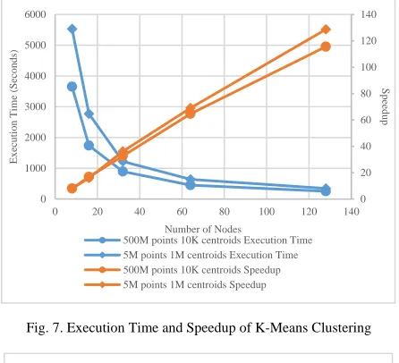
We run K-Means clustering with two different generated random data sets. One is clustering 500 million 3D points into ten thousand clusters, while another is clustering 5 million 3D points into 1 million clusters. In the former, the input data is about 12 GB and the ratio of points to clusters is 50000:1. In the larger case, the input data size is only about 120 MB but the ratio is 5:1. Such a ratio is commonly high in clustering but the low ratio is used in a different scenario where the algorithm tries to do fine-grained clustering as classification [32] [33]. Because each point is required to calculate distance with all the cluster centers, total workload of the two tests are similar.

Fig. 7. Due to the cache effect, we see “5 million points and 1 million centroids” is slower than “500 million points and 10 thousand centroids” when the number of nodes is small. But as the number of nodes increases, they draw closer to one another. For speedup, we assume we have the linear speedup on the smallest number of nodes we test. So we consider the speedup on 8 nodes is 8. The experiments show the speedup comparison in both test cases is close to linear.

C. Results on Force-directed Graph Drawing Algorithm This algorithm runs with a graph of 477,111 vertices and 665,599 undirected edges. The graph represents a retweet network about the presidential election in 2012 from Twitter [34].

Although the size of input data is fairly small, the algorithm is computation intensive. We load vertex ID as ‘int’ and initial random coordination values as ‘float’. The total size is about 16M. We test the algorithm on 1 node as the base case and then scale to 8, 16, 32, 64 and 128 nodes. Execution time of 20 iterations and speedup are shown in Fig. 8. From 1 node to 16 nodes, we observe almost linear speedup. It drops smoothly after 32 nodes. On 128 nodes, because the computation time per iteration slows to around 3 seconds, the speedup drops sharply.

D. Results on WDA-SMACOF

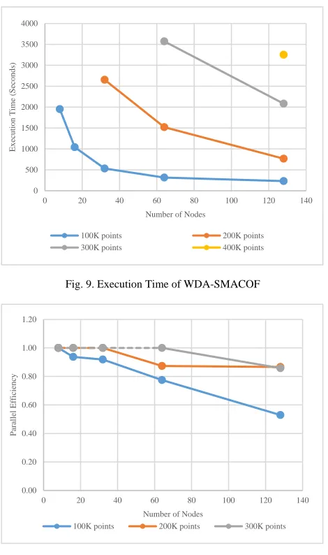
The WDA-SMACOF algorithm runs with different problem sizes including 100K points, 200K points, 300K points and 400K points. Each point represents a gene sequence in a dataset of representative 454 pyrosequence from spores of known AM fungal species [28]. Because the input data is the distance matrix of points and related weight matrix and V matrix, the total size of input data is in quadratic growth. We cache distance matrix in short arrays, weight matrix in double arrays and V matrix in int arrays. Then the total size of input data is about 140 GB for 100K problem, about 560 GB for 200K problem, 1.3 TB for 300K problem and 2.2 TB for 400K problem.

The input data is stored in DC2 and each matrix is split into 4096 files. They are loaded from there to workers. Due to memory limitations, the minimum number of nodes required to run the 100K problem is 8. Then we scale 100K problems on 8, 16, 32, 64 and 128 nodes. But for the 200K problem, the minimum number of nodes required is 32. So we scale the 200K problem on 32, 64 and 128 nodes. With the 300K problem, the minimum node requirement is 64, so we scale 300K problems from 64 to 128 nodes. Lastly for the 400K problem, we only run it on 128 nodes because this is the minimum requirement for that amount.

Here we give the execution time, parallel efficiency and speedup (see Fig. 9, Fig. 10, Fig. 11). Because we cannot run each input on a single machine, we choose the minimum number of nodes to run the job as the base to calculate parallel efficiency and speedup. In most cases, the efficiency values are very good. The only point that has low efficiency is 100K problems on 128 nodes. This is a standard effect in parallel computing where the small problem size reduces compute time compared to communication which in this case has an

overhead of about 40% of total execution time, and the overall efficiency drops.

VII. CONCLUSION

In this paper, we investigate basic architecture issues and the challenges of data analysis tools for complex scientific applications. Based on our analysis of different big data tools, we propose to abstract a collective communication layer from these computation models. We build Map-Collective as a unified model to improve the performance and expressiveness of big data tools.

With three applications K-Means Clustering, Force-directed Graph Drawing and WDA-SMACOF, we demonstrate that the Map-Collective model can be simply expressed with the combination of proposed collective communication abstractions. The experiments show that we can scale these applications to 128 nodes with 4096 processors on the Big Red II supercomputer, where the speedup in most tests is close to linear and we’re looking at running it at much larger scales.

Map-Collective [12][25] communication layer is designed in a pluggable, infrastructure agnostic way. It can be used in Hadoop ecosystem and HPC system. Harp has an open source

Fig. 7. Execution Time and Speedup of K-Means Clustering

Fig. 8. Execution Time and Speedup of Force-Directed Graph Drawing Algorithm 0 20 40 60 80 100 120 140 0 1000 2000 3000 4000 5000 6000

0 20 40 60 80 100 120 140

S pe edup E x ec ut ion T im e (S ec onds )

Number of Nodes

500M points 10K centroids Execution Time 5M points 1M centroids Execution Time 500M points 10K centroids Speedup 5M points 1M centroids Speedup

0 10 20 30 40 50 60 70 80 90 0 1000 2000 3000 4000 5000 6000 7000 8000

0 20 40 60 80 100 120 140

S pe edup E x ec ut ion T im e (S ec onds )

Number of Nodes

collective communication library that can be plugged into Hadoop. With this plug-in, Map-Reduce jobs can be transformed into Map-Collective jobs and users can invoke efficient in memory message passing operations such as

collective communication (e.g. broadcast and group-by) and point-to-point communication directly within Map tasks. For the first time, Map-Collective brings high performance to the Apache Big Data Stack in a clear communication abstraction, which did not exist before in the Hadoop ecosystem. We expect Harp to equal MPI performance with straightforward optimizations. Note that these ideas will allow simple modifications of Mahout library that will drastically improve the typical low parallel performance of Mahout; this demonstrates value of building new abstractions into Hadoop rather than developing a totally new infrastructure as we did in our prototype Twister system.

Future work will also look at including the high performance dataflow communication libraries being developed for simulation (exascale) and incorporate them as implementations in the Map-Collective abstraction. We will extend the work on fault tolerance to evaluate the current best practice in MPI, Spark and Hadoop. We are working with several application groups and will extend the data abstractions to for example include those needed in pixel and spatial problems.

ACKNOWLEDGEMENT

We appreciate the system support offered by Big Red II. We gratefully acknowledge support from National Science Foundation grant OCI-1149432.

REFERENCES

[1] J. Dean and S. Ghemawat. “Mapreduce: Simplified data processing on large clusters.” OSDI, 2004.

[2] Apache Hadoop. http://hadoop.apache.org

[3] J. Ekanayake, H. Li, B. Zhang, T. Gunarathne, S.-H, Bae, J. Qiu, G. Fox. “Twister: A Runtime for iterative MapReduce.” Workshop on MapReduce and its Applications, HPDC, 2010.

[4] Y. Bu, B. Howe, M. Balazinska, and M. Ernst. “Haloop: Efficient Iterative Data Processing on Large Clusters”. VLDB, 2010.

[5] M. Zaharia, M. Chowdhury, M. J. Franklin, S. Shenker, and I. Stoica. “Spark: Cluster Computing with Working Sets”. HotCloud, 2010. [6] Grzegorz Malewicz, et al. “Pregel: A System for Large-scale Graph

Processing”. SIGMOD. 2010.

[7] Apache Giraph. https://giraph.apache.org/ [8] Apache Hama. https://hama.apache.org/

[9] J. MacQueen, “Some Methods for Classification and Analysis of MultiVariate Observations.” Berkeley Symp. On Mathematical Statistics and Probability, 1967.

[10] S. Lloyd. “Least Squares Quantization in PCM”. IEEE Transactions on Information Theory 28 (2): 129–137, 1982.

[11] Apache Mahout. https://mahout.apache.org/

[12] J. Qiu, B. Zhang, “Mammoth Data in the Cloud: Clustering Social Images.” In Clouds, Grids and Big Data, IOS Press, 2013.

[13] B. Zhang, J. Qiu. “High Performance Clustering of Social Images in a Map-Collective Programming Model”. Poster in proceedings of ACM Symposium On Cloud Computing, 2013.

[14] E. Chan, M. Heimlich, A. Purkayastha, and R. Geijn. “Collective communication: theory, practice, and experience”. Concurrency and Computation: Practice and Experience (19), 2007.

[15] MPI Forum. “MPI: A Message Passing Interface”. In Proceedings of Supercomputing, 1993.

[16] MPICH2-YARN. https://github.com/clarkyzl/mpich2-yarn

[17] Y. Low, et al. “GraphLab: A New Parallel Framework for Machine Learning”. Conference on Uncertainty in Artificial Intelligence, 2010. Fig. 9. Execution Time of WDA-SMACOF

Fig. 10. Parallel Efficiency of WDA-SMACOF

Fig. 11. Speedup of WDA-SMACOF

0 500 1000 1500 2000 2500 3000 3500 4000

0 20 40 60 80 100 120 140

E

x

ec

ut

ion T

im

e

(S

ec

onds

)

Number of Nodes

100K points 200K points

300K points 400K points

0.00 0.20 0.40 0.60 0.80 1.00 1.20

0 20 40 60 80 100 120 140

P

ar

al

lel

E

ff

ici

en

cy

Number of Nodes

100K points 200K points 300K points

0 20 40 60 80 100 120

0 20 40 60 80 100 120 140

S

pe

edup

Number of Nodes

[18] Y. Low, et al. “Distributed GraphLab: A Framework for Machine Learning and Data Mining in the Cloud”. PVLDB, 2012.

[19] J. Gonzalez, et al. “PowerGraph: Distributed Graph-Parallel Computation on Natural Graphs”. OSDI, 2012.

[20] R. Xin, et al. “GraphX: A Resilient Distributed Graph System on Spark”. GRADES, SIGMOD workshop, 2013.

[21] M. Isard et al. “Dryad: Distributed Data-Parallel Programs from Sequential Building Blocks”. EuroSys, 2007.

[22] Stratosphere. http://stratosphere.eu/ [23] REEF. http://www.reef-project.org/

[24] M. Chowdhury et al. “Managing Data Transfers in Computer Clusters with Orchestra”. ACM SIGCOM, 2011.

[25] T. Gunarathne, J. Qiu, D. Gannon, “Towards a Collective Layer in the Big Data Stack”. The proceedings of the 14th IEEE/ACM International Symposium on Cluster, Cloud and Grid Computing Conference, 2014. [26] T. Fruchterman, and M. Reingold. “Graph Drawing by Force-Directed

Placement”, Software – Practice & Experience 21 (11): 1129–1164, 1991.

[27] Y. Ruan. “A Robust and Scalable Solution for Interpolative Multidimensional Scaling With Weighting”. E-Science, 2013.

[28] Y. Ruan, G. House, S. Ekanayake, U. Schütte, J. Bever, H. Tang, G. Fox. “Integration of Clustering and Multidimensional Scaling to Determine Phylogenetic Trees as Spherical Phylograms Visualized in 3 Dimensions”. Proceedings of C4Bio of IEEE/ACM CCGrid, 2014. [29] Y. Ruan, et al. “DACIDR: Deterministic Annealed Clustering with

Interpolative Dimension Reduction using a Large Collection of 16S rRNA Sequences”. Proceedings of ACM-BCB, 2012.

[30] Y. Ruan, et al. “HyMR: a Hybrid MapReduce Workflow System”. Proceedings of ECMLS’12 of ACM HPDC, 2012

[31] Big Red II. https://kb.iu.edu/data/bcqt.html

[32] G. Fox. “Robust Scalable Visualized Clustering in Vector and non Vector Semimetric Spaces”. Parallel Processing Letters 23, 2013. [33] G. Fox, D. Mani. “Parallel Deterministic Annealing Clustering and Its

Application to LC-MS Data Analysis”. Big Data, 2013.