Parallel LDA Through Synchronized
Communication Optimizations
Bingjing Zhang
∗, Bo Peng
∗†, Judy Qiu
∗∗ School of Informatics and Computing, Indiana University, Bloomington, IN, USA
†Computer Science Department of Peking University, Beijing, China
zhangbj, pengb, [email protected]
Abstract—Sophisticated big data machine learning applications
are difficult to parallelize because it not only needs to process a big training dataset, it also needs to synchronize big model data in iterations. In parallel LDA, comparing synchronized and asynchronous communication methods under data parallelism and model parallelism, we note that the power-law distribution of word counts in LDA training datasets suggests using synchro-nized communication optimizations can improve the efficiency of the model update to allow the model to converge faster, shrink the model size, and further reduce the computation time in later iterations. Therefore, we abstracted new synchronized communication operations and developed two new parallel LDA implementations “lda-lgs” and “lda-rtt”. We compare our new approaches to leading implementations in the field on an Intel Haswell cluster with 100 nodes, 4000 threads. In data parallelism, “lda-lgs” can reach higher model likelihood with shorter or similar execution time compared with Yahoo! LDA. In model parallelism, when achieving similar model likelihood, “lda-rtt” can run up to 3.9 times faster compared with Petuum LDA.
I. INTRODUCTION
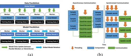
One challenge of parallel machine learning applications is while training data can be split among parallel workers, the model data all local computations depend on is growing pro-gressively and generates significant synchronization overhead. Currently two types of parallelism are commonly used to solve this problem (see Fig. 1a):
Data Parallelism While the training data are split among
parallel workers, the global model is distributed on a set of servers or existing parallel workers. Each worker computes on a local model and updates it with the synchronization between local models and the global model.
Model Parallelism In addition to splitting the training data
over parallel workers, the global model data is split between parallel workers and rotated during sampling.
Latent Dirichlet Allocation (LDA) [1] is an important ma-chine learning technology that has been widely used in many areas such as text mining, advertising, recommender systems, network analysis, and genetics. Though extensive research on this topic exists, people are endeavoring to scale it to web-scale corpora with big models to explore more subtle semantics. We have identified the importance of model synchronization or update speed and observed that a fast communication method can speed up convergence rate, subsequently reduce the model size and shorten computation time in later iterations. Although the proposed synchronized and asynchronous approaches in Fig. 1b both cause the model to converge without affecting
Training Data 1
Local Model
Global Model
Training Data 2
Local Model
Training Data 3
Local Model
Training Data 4
Local Model Worker
Training Data 1 Global Model 1
Training Data 2 Global Model 2
Training Data 3 Global Model 3
Training Data 4 Global Model 4
Data Parallelism
Worker Worker Worker
Model Parallelism
Worker
Worker Worker Worker
Model Data Update between
Parallel Workers or Client/Server Global Model Rotation
(a)
Sample a word
Sample a word Send the word
Send the word
Sample words
Sample words Update words
Update words Sample
a word
Sample a word
Send the word
Send the word
Asynchronous Communication Synchronized Communication
Time
Threading Computation Communication
Sample words
Update words Sample
a word
Sample a word
Send the word
Send the word
(b)
Fig. 1. (a) Data Parallelism vs. Model Parallelism and (b) Asynchronous Communication vs. Synchronized Communication in LDA
the correctness of the algorithm, it is often unclear which strategy performs better for LDA applications. Asynchronous communication is popular because it avoids a global waiting overhead between parallel workers as well as local waiting between computation threads and communication threads. In data parallelism, asynchronous communication allows local computation to continue without waiting for the completion of updates on the global model from all parallel workers per iteration. In model parallelism, although model rotation is synchronized, per word sampling and sending can overlap without waiting on each worker, exemplified by asynchronous communication.
After analyzing the characteristics of LDA training datasets, it becomes clear that the counts of each word in the training documents fall under the power-law distribution. As a result, when data parallelism is used, many words in the global model will display on all the workers’ local models, which forms “one-to-all” communication patterns for synchroniza-tion. Likewise, in model parallelism, as the size of the global model data expands, each worker handles more data transfer. These observations imply that routing optimized synchronized communication operations can be used to improve LDA model update speed.
[image:1.612.325.551.202.299.2]can-not abstract the local/global model synchronization in data parallelism or the model rotation in model parallelism. As such, we abstracted three other communication patterns named “syncLocalWithGlobal”, “syncGlobalWithLocal”, and “rotateGlobal”. The new patterns are generalizable and can be applied to LDA as well as many other machine learning ap-plications. We implemented one LDA application which uses “syncLocalWithGlobal” and “syncGlobalWithLocal” to per-form data parallelism and another which uses “rotateGlobal” to perform model parallelism. We compared our implemen-tations with a set of state-of-the-art implemenimplemen-tations based on asynchronous communication methods, such as Yahoo! LDA [3] and Petuum LDA [4], on several datasets with a total of 10 billion model parameters. We conduct extensive performance experiments on Intel Haswell architecture up to 100 nodes with a total of 4000 parallel threads. The results show that synchronized communication optimizations can significantly reduce communication overhead and improve model convergence speed.
The following sections describe: the cost model of LDA algorithm (Section 2), synchronized communication methods (Section 3), implementations of Harp-LDA (Section 4), per-formance results of our implementations (Section 5), related work (Section 6), and conclusions (Section 7).
II. COSTMODEL
A. LDA model
LDA is a generative probabilistic data modeling technique. Training data are abstracted as a document collection where each document is a bag of words. LDA models the data by introducing latent topics, which tries to capture the underlining semantic connections and structures inside the data. In LDA model, a document is a mixture of latent topics, and each topic is a multinomial distribution over words. In the generative
process, for document j, we first draw a topic distribution θj
from a Dirichlet with parameter α. Then for each wordi in
this document, we draw a topiczij=kfrom the multinomial
distribution with parameterθj. Finally, wordxijis drawn from
a multinomial φwk|k=zij, which also derives from a Dirichlet
with parameterβ. Here, the wordsxij are observed variables,
θ,φ,zare latent variables, andαandβ are hyper parameters.
The purpose of LDA inference is to compute the posterior distribution of latent variables given the observed variables. Many approximate inference algorithms exist. In a practice on big data, Collapsed Gibbs Sampling (CGS) [5] shows high scalability. It is a kind of Markov Chain Monte Carlo algorithm which has three phases, the initialize, burn-in, and stationary phase.
In the initialize phase, each word is assigned a random topic
denoted as zij. Then it begins to reassign topics to each word
wij according to the conditional probability ofzij, which is
henceforth called sampling.
p zij =k|z¬ij, x, α, β
∝ N
¬ij
wk +β
P
wN
¬ij
wk +V β
Nkj¬ij+α
(1)
Here, superscript ¬ij means that the corresponding word is
excluded in the counts.V is vocabulary size.Nwk is the count
of word w assigned to topick, andNkjis the count of topick
assigned in document j, which are sufficient statistics for the
latent variableθandφ. The latent variables can be represented
by three matrices Zij, Nwk andNkj, which are model data.
Intuitively, by equation(1), with higher probability a word will be assigned to the topic that has been assigned to it’s co-occurring words. Therefore, sampling by the latest model data of co-occurring words is critical for convergence, and that is why synchronization is so important in a parallel LDA trainer.
Hyper parameters α and β are also called concentration
parameters, which control the topic density in the final model.
The larger theαandβ, the more topics can be drawn into a
document and assigned to a word, and the more non-zero cells
in each row of theNwk andNkj matrices. Although a useful
LDA trainer often has the feature of α and β optimization
dynamically tuned to fit the training data, in this paper, we
skip such a feature and use symmetricαandβ both fixed to
a common used value 0.01 to exclude the complex effects on performance caused by their dynamics.
Latent variables will gradually converge in the process of iterative sampling. This is the phase where burn-in occurs and finally reaches the stationary state. From that point, we can draw samples from the sampling process and use them to calculate the posterior distribution.
To evaluate the quality of the final model learned by LDA, held-out testsets are often used, taking likelihood or perplexity as the accuracy metrics. In this paper, we only use the model data likelihood on the training dataset to monitor the convergence of the LDA trainer, which is consistent with the held-out testset results in our experiments, only much faster.
Sampling on zij in CGS is a strictly sequential process.
AD-LDA [6] is the seminal work allowing us to relax this se-quential sampling requirement. It assumes that the dependence
between one topic assignment zij and another zij is weak
in that different words in different documents are sampled concurrently. In AD-LDA, training data are partitioned into n subsets, with n Gibbs Samplers running parallel on each collection, and the samplers synchronize their model data with others at certain time points. This parallel version produces a useful model, establishing the foundation of large-scale parallel CGS implementations of LDA trainers.
B. Performance Factors
Sampling Algorithm Computation complexity of a
sam-pling algorithm basically determines the overall performance.
Although there is aO(1) sampling algorithm, LightLDA [7],
proposed in the literature, we focus on SparseLDA [8], which is an optimized CGS sampling algorithm mostly used in the state-of-the-art LDA trainers, in order to make a broader comparison. SparseLDA splits the equation (1) into three parts:
p(zij=k|rest)∝
Nwk¬ij(Nkj¬ij+α) +β∗Nkj¬ij+αβ P
wN
¬ij
wk +V β
The denominator is a constant when sampling on one word. The third part of the numerator is also a constant; the second
part is non-zero only whenNkjis non-zero, and the first part is
non-zero only whenNwk is non-zero. In naive CGS sampling,
the conditional probability will compute K times, while in
SparseLDA, the computation can be decreased to non-zero
items number inNwk andNkj, which are much smaller than
K on average.
We found that in practice, the sampling performance is more memory bounded than computation bounded, since the computation is very simple and memory access to two large matrices is not by its nature cache friendly. Furthermore, CGS has a feature of exchangeability that permits the order of word sampling to be changed. In practice, sampling can take the order by row or column on the document-word matrix. Equation(2) is the form optimized for row order, called
sample-by-doc. In this case,Nkj can be cached for the words
in the same row, and the computation complexity in terms of
amortized random memory access time is O(P
k1(Nwk 6=
0)). Symmetrically, sample-by-word will have the complexity
of O(P
k1(Nkj6= 0)).
Parallelism Strategy Data partition on the training data,
which is a document-word matrix, can be done either in the rows or the columns. If data are partitioned by rows, each
subset data has its localz,Nkj,Nwkmodel data and onlyNwk
needs to be synchronized with others. In general applications, the row number is much larger than the column number, so partition by rows will generate a smaller model data size. We only refer to the shared word-topic matrix as model data.
There are many possible communication strategies which control how to do model data synchronization between parallel workers. Modern clusters allow two levels of parallelism: inter-node and intra-inter-node parallelism. In this paper, we focus on inter-node parallelism by exploring the differences between the communication strategies.
Cluster configurations include nodes numberNand network
bandwidth B, memory size M for each node, and thread
number T for each node. As many-core technology brings
forth more powerful machines to bear complicated compu-tation applications, large-scale machine learning applications
will benefit from relatively small numbers of N with a large
number of T to achieve high scale parallelism.
Data Property Training data can be characterized by the
total numbers of tokens, denoted as W, and the number of
documents, denoted as D. The model data Nwk is a V ∗K
matrix andNkj is aD∗K matrix, whereV is the vocabulary
size and K is the topic number.
LDA is an iterative algorithm. It keeps sampling on the training data and updating (synchronizing) the model data until it converges. One iteration equals one round of sampling the training data and in one synchronization pass all the model data are synchronized. As we described above, both parts are highly related to the model data size, not in terms of the matrix dimension but instead the non-zero items count.
C. Model Data
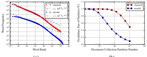
Model Size Power law distribution is a general
phe-nomenon. It has another equal form for text data, Zipf’s law, where the frequency of a word is proportional to the reciprocal of its rank.
f req(i) =C∗i−λ (3)
Here,iis word rank, and λis near 1.
There are a total of V unique words in the training data.
We then have:
W =
V
X
i=1
(f req(i))) =
V
X
i=1
(C∗i−λ)
≈C∗(ln(V) +γ+ 1
2V) (4)
Ifλis 1, this is the partial sum of harmonic series which have
logarithmic growth, whereγ is the EulerMascheroni constant
≈0.57721.
Model data, V ∗K, is a big but sparse matrix. In general,
V is 1M, K is 1K, while for big models it can even reach
1M*1M. The non-zero cell count of the matrix is the actual
model size, denoted asS,S << V ∗K.
In the initialization of CGS, word-topic count matrix is initialized by random topic assignment for each word. So the
word i will getmax(K, f req(i))non-zero cells. Iff req(J) =
K,J =C/K, we get:
Sinit= J
X
i=1
K+
V
X
i=J+1
f req(i) =W −
J
X
i=1
f req(i) +
J
X
i=1
K
=C∗(lnV +lnK−lnC+ 1) (5)
The actual model sizeSinitis logarithmic to matrix sizeV∗K.
This does not mean Sinit is small, since the constant C =
f req(1)can be very large; even C∗ln(V ∗K)can be huge.
An increase of dimension in the model will not increase the model data size dramatically.
With the progress of iterations and algorithm convergence, the model data size will shrink. The concentration parameters
α and β control the final sparsity of the topic distribution.
When a stationary state is reached, the average count value will
drop to a certain small constant ratio ofK, with the constant
δdetermined by the properties of the training data itself.
Sf inal=mean(word−topiccount)∗V =δ∗K∗V (6)
Model Data Partition After training data is partitioned to
each node of the cluster, a local model dataS0will be built up
and used in local computation. This local model data should
synchronize with global model data S frequently to make
the training process converge. In fact, the synchronization frequency is highly relevant to the final model accuracy.
This data partition strategy can decrease local training data
W0 linear to node numberN. Therefore, we getW0=W/N.
For computations proportional to the total word numberW0,
100 101 102 103 104 105 106 107
Word Rank
100
101
102
103
104
105
106
107
108
109
1010
W
ord
Frequenc
y
clueweb
y=109.9x−0.9
enwiki
y=107.4x−0.8
(a)
100 101 102 103 104
Document Collection Partition Number
0.0 0.2 0.4 0.6 0.8 1.0 1.2
Vocab
ulary
Size
of
Partition
(%) cluewebenwiki
[image:4.612.57.291.61.153.2](b)
Fig. 2. Model Size of (a) Zipf’s Law and (b) Vocabulary and Data Partition
we have, the better performance we can expect. Assuming
C0 =C/N, the actual local model size S0
init is:
Sinit0 =C
0
∗(lnV0+lnK−lnC0+ 1)
≤ NC(lnV +lnK−lnC+ 1 +lnN)
≤ NS +C
NlnN (7)
In general configurations lnN is smaller thanlnV +lnK−
lnC+1, so local model sizeS0
initis no more than
2
NSinit. The
initialized local model data size is controlled by data partitions. When model data synchronization begins, all words in the local vocabulary need to fetch the corresponding global model
data. The local vocabulary size V0 will then determine both
the communication data volume and local model size in the burn-in phase, which becomes the problem.
It is clear that when documents are partitioned to N
nodes, every word with a frequency larger than N will get
a high probability occurring on each node. If at rank L,
f req(L) = N, we get: L = W
(lnV+γ)∗N. On the “enwiki”
dataset, W=1B,V=1M, N=100, we get L = 0.69V; on the
“clueweb” dataset, W=10B, V=1M, N=100, L > V. For a
reasonably large training dataset, L is easily larger than V,
which means it needs to send/receive and hold almost all the global model data locally.
In sum, because of the power-law distribution in the training data, data parallelism can help distribute training data among nodes and parallelize the computation tasks accordingly, but it cannot effectively control the volume of the model data transferred between nodes. When dealing with larger data and larger models, simply deploying more nodes will not prove an effective solution, for model data synchronization will eventually become a bottleneck.
D. Experiments
We first validate Zipf’s law of word distribution on “clueweb” and “enwiki” datasets, where the top 1M most frequent words are selected (see Fig. 2a). They both show considerable matching results, especially in the word region with high frequency. In the preprocess step for the LDA trainer, stop words and low frequency words are often removed. This results in a flatter slope and a denser model than expected from equation(5). In Fig. 2b, we represent the difficulty of
controlling the vocabulary size by random partition of docu-ment collection. When 10 times more partitions are introduced, there is only a sub-linear portion decrease of the vocabulary size in each partition compared to the total one; e.g. on the “clueweb” dataset, each partition gets 92.5% vocabulary size when data is randomly distributed to 128 nodes. The “enwiki” dataset is about 12 times smaller than “clueweb”, and it gets 90% at 8 nodes, keeping a similar ratio. This figure shows that local models will not be of the same size as the global one, although not much smaller.
III. SYNCHRONIZEDCOMMUNICATIONMETHODS
Past research has shown that collective communication op-erations are indispensable in iteration-based machine learning algorithms. Chu et al. [9] mentions that many machine learn-ing algorithms can be implemented in MapReduce systems [10]. The underlying principle of this conclusion is that each iteration in the algorithm is dependent on the synchronization of the local models computed on each worker at the last iteration. However, MapReduce systems only provide a fixed “shuffling” communication pattern. Thus, in Harp, a separate collective communication abstraction layer provides a set of data abstractions and related collective communication opera-tion abstracopera-tions.
For LDA, both data parallelism and model parallelism ben-efit from synchronized communication optimizations. In data parallelism, “one-to-all” communication patterns play a crucial role in the synchronization to enable the optimization of the communication performance with collective communication operations. In model parallelism, using collective communi-cation can maximize bandwidth usage between a worker and its neighbors and reduce network conflicts in rotating model partitions.
A. The Abstraction Of Global/Local Data Synchronization
Considering the sparsity of the local model data distribution on workers, collective communication optimization, and the existing collective communication abstractions in Harp, we added two other data abstractions and related new collective communication operations.
The two types of data abstractions are the global table and the local table. The concept “table” has been defined in previous Harp collective communication abstractions [2]. Each table may contain one or more partitions, and the tables defined on different workers are associated in order to manage a distributed dataset. In global tables, each partition has a unique ID and represents a part of the whole distributed dataset; but in local tables, partitions on different workers can share the same partition ID. Each of these partitions sharing the same ID is considered a local version of a partition in the full distributed dataset.
Secondly, “syncLocalWithGlobal” uses the data in global tables to synchronize local tables. Based on the needs of partitions in local tables, this operation will redistribute the partitions in the global table to local tables. If one partition is required by all the workers, it will be broadcasted.
Lastly, “rotateGlobal” will consider workers in a ring topol-ogy and shift the partitions in the global table owned by one worker to the right neighbor worker and then receive the partitions from the left neighbor. When the operation is completed, the contents of the distributed dataset in the global tables won’t change, but each worker will hold a different set of partitions. Since each worker only talks to its neighbors, “rotateGlobal” can transmit global data in parallel without any network conflicts.
B. The Applicability of Synchronized Communication Methods
“syncGlobalWithLocal” and “syncLocalWithGlobal” are abstracted from data parallelism, and “rotateGlobal” is ab-stracted from model parallelism. As a result, they can be applied to many other machine learning applications with big model data.
Here we simply discuss the applicability of these methods based on the computation dependency in the applications. We draw a matrix to describe each worker’s requirements on the global model data in the parallel computation per iteration. In this matrix, each row represents a worker, each column represents a global data partition, and each element shows the requirements of the partition in the local compu-tation. Based on the density of this matrix, we can choose proper operations in different applications. If the matrix is dense, we suggest using the “rotateGlobal” operation. Using k-means clustering as an example, the global model data are the centroids, and the local computation needs all the centroids data. Thus “rotateGlobal” allows each worker to access all the centroids data efficiently. If the matrix is sparse, using “syncGlobalWithLocal” and “syncLocalWithGlobal” is a superior solution. For example, in graph algorithms such as PageRank, the global model data are the vertices’ page-rank values and counts of out-edges. The local computa-tion goes through edges and calculates the partial result of the new page-rank values. Then “syncGlobalWithLocal” and “syncLocalWithGlobal” can be used to synchronize global page-rank values.
IV. HARP-LDA IMPLEMENTATION
A. Training Data Partitioning and Model Data Initialization
For the training data, we split the documents into files evenly. For the model data, since words with high frequency can dominate the computation and communication, we parti-tion the global model based on the frequency of words in the training dataset. During the preprocessing of the training data, each word is given an ID based on their frequency starting from 0. The lower the occurrence of the word, the higher the ID. Then we partition the words’ topic counts using
range-based partitioning. Assuming each partition containsmwords,
Partition 0 contains words with IDs from 0 to m−1, and
Training Data
1 Load Worker Worker Worker
Sync
4
Global Model 2
Compute
2
Global Model 3
Compute
2 Global
Model 1
Compute
2
3 3 Sync Sync
3
Iteration
Local Model
Local Model
Local Model
Worker Worker
Worker
Rotate
Global Model 2
Compute
2
Global Model 3
Compute
2 Global
Model 1
Compute
2
3
3 Rotate
Rotate
3
lda-lgs (use syncLocalWithGlobal
& syncGlobalWithLocal)
lda-rtt (use rotateGlobal)
Fig. 3. Inter-node Parallelism (data loadinghstep 1iand iterationhstep 4i
are common procedures for both implementations)
Partition 1 contains words with IDs fromm to2m−1, and
so on. As a result, the partitions with low IDs contain the words with the highest frequency. The initial global model is generated by randomly assigning each token to a topic and aggregated through “syncGlobalWithLocal”. The mapping between partition IDs and worker IDs is calculated based on
the modulo operation. Assuming there is a worker with IDw
among a total of N workers, the partitions contained on this
worker are Partitionw, Partitionw+N, Partitionw+2N, and
so on. In this way, each worker contains a number of words whose frequencies rank from high to low.
B. Inter-node Parallelism
During iterations of the sampling, we use two different approaches to update the global model which results in two im-plementations (See Fig. 3). One implementation, named “lda-lgs”, follows data parallelism and uses “syncGlobalWithLocal” paired with “syncLocalWithGlobal” operations. The other im-plementation, named “lda-rtt”, follows model parallelism and uses “rotateGlobal” operation.
C. Overlap Communication with Computation
Synchronized communication is commonly criticized for generating much overhead and making all workers wait for the completion of synchronization. We approached this problem in three steps. The first step is to balance the communication load on each worker through partitioning the global model based on word frequencies. The second step is to improve the speed with optimized collective communication. Here we discuss the third step, which is overlapping computation and communication in execution.
In “lda-rtt”, we slice the global model partitions held on each worker into two sets. Slicing is conducted by first sorting the partition IDs in ascending order and then assigning the partitions to the two slices in alternate order. As a result, each slice will contain words with both high and low frequencies. During the sampling, when a worker finishes processing the first slice, it uses another thread to rotate this slice and simultaneously continues processing the second slice. Once the second slice is processed, the first slice may be ready for further processing. After both slices have finished a round of rotation, the sampling of an iteration is completed. The overlapping between computation and communication occurs when the worker processes one slice and rotates another slice at the same time.
In “lda-lgs”, we split the local data table into two slices. During the sampling, when each worker samples a slice, it requests another thread to synchronize the other slice through “syncLocalWithGlobal” and “syncGlobalWithLocal” operations. We map partitions based on their IDs into slices so that local partitions with the same IDs are guaranteed to be synchronized in iterations.
D. Intra-node Parallelism
In Harp-LDA, we use the “Computation” component to manage multi-threading sampling within one worker. The sampling process follows a SparseLDA algorithm and can be performed in two ways. One approach is to go through each document and sample the topics of every token. The other approach is to go through each word and sample the topics for word occurrences in each document. To keep the sam-pling order consistent between implementations for unbiased performance comparisons in future experiments, we sample topics by documents in “lda-lgs” as Yahoo! LDA and sample topics by words in “lda-rtt” as Petuum LDA. Note that when sampling topics by words, we balance the computation load by assigning words to threads based on their frequencies.
The local model is shared between threads. When sampling topics by documents, the word-topic model is required to access with locks. Symmetrically, when sampling topics by words, the document-topic model is required to access with locks. We provide a read lock and a write lock on each document/word’s topic count map. Before sampling, a token’s document/word topic counts are read out, and after sampling, the updates are written back. If the next token for sampling is the same word, the sampling thread will keep using the thread local cached topic counts to avoid repeating fetching the shared
data. During the update, we separate “updating an existing topic entry” and “adding a count to a new topic entry”. In “updating an existing topic entry”, because the map structure is not altered during updating and reading a primitive integer is an atomic operation in modern x86 architecture, it is safe to execute “read” and “update” concurrently with a shared read lock. However, in order to ensure the correctness of the topic count values, “update” operations are still required to be exclusive. In the operation of “adding a count to a new topic entry”, since the map structure is modified, we have to use a write lock.
Though the concurrency is greatly improved, our current implementation is still slower compared with Yahoo! LDA and Petuum in the first iteration of sampling. This could be caused by the difference in the implementation language (Java/C++) and the performance of the data structure (primitive int based hashmap [12]/primitive int array). As many-core architecture is becoming more common, high performance concurrent sam-pling with many-threads is a challenge to all implementations. However, in this paper our aim is not to provide the fastest LDA implementation but to show the advantages of using synchronized communication methods in LDA model conver-gence compared with asynchronous communication methods.
V. EXPERIMENTS
A. Experiment Settings
Experiments were done on the Juliet Intel Haswell cluster [13], which contains 32 18-core 72-thread nodes and 96 24-core 48-thread nodes. All the nodes have 128GB memory and are connected with two types of networks: 1Gbps Ethernet (eth) and Infiniband (ib). For testing, we use 31 18-core nodes and 69 24-core nodes to form a cluster of 100 nodes with 40 threads each for computation. Most tests are done with Infiniband through IPoIB support unless otherwise specified.
Several datasets are used (see Table I). The total number
of model parameters is kept as 10 billion on all datasets. α
andβ are both fixed at 0.01. We test several implementations
(see Table II) on these datasets. We compare synchronized communication methods with asynchronous communication methods on both model parallelism and data parallelism. By studying the convergence speed and execution time, we learned how the difference in communication methods affects the performance of LDA.
B. Convergence Speed Per Iteration
First, we compare the convergence speed of the LDA word-topic model on iterations by analyzing model results learned on iterations 1, 10, 20, 30... 200. It is fair to use iterations to measure the performance of model convergence because it does not consider the performance difference in execution.
TABLE I
TRAININGDATASETTINGSUSEDINTHEEXPERIMENTS
Dataset enwiki clueweb bi-gram gutenberg
Num. of Docs 3.8M 50.5M 3.9M 26.2K
Num. of Tokens 1.1B 12.4B 1.7B 836.8M
Vocabulary 1M 1M 20M 1M
Doc Len.
AVG/STD 293/523 224/352 434/776 31879/42147
Lowest Word
Freq. 7 285 6 2
Num. of Topics 10K 10K 500 10K
Init. Model Size 2.0GB 14.7GB 5.9GB 1.7GB
Note: Both “enwiki” and “bi-gram” are English articles from Wikipedia [14]. “clueweb” is a 10% dataset from ClueWeb09, which is a collection of English web pages [15]. “gutenberg” is comprised of English books from Project GutenBurg [16].
TABLE II
LDA IMPLEMENTATIONSUSEDINTHEEXPERIMENTS
DATA PARALLELISM
lgs - “lda-lgs” impl. with no routing optimization- Slower than “lgs-opt”
lgs-opt
- “lgs” with routing optimization
- Faster than Yahoo! LDA on “enwiki” with higher model likelihood
lgs-opt-4s
- “lgs-opt” with 4 rounds of model synchronization per iteration; each round uses 1/4 of the training data - Performance comparable to Yahoo! LDA on “clueweb” with higher model likelihood
Yahoo!
LDA - Master branch on GitHub [3]
MODEL PARALLELISM
rtt
- “lda-rtt” impl.
- Speed comparable with Petuum on “clueweb” but 3.9 times faster on “bi-gram” and 5.4 times faster on “gutenbuerg”
Petuum - Version 1.1 [4]
Note: Our implementations are indicated in bold.
overlapped. In contrast to “lgs-opt”, the convergence speed of “lgs-opt-4s” is as high as Petuum. This shows that increasing the rounds of model synchronization thereby increases the convergence speed. Yahoo! LDA has the slowest convergence speed because asynchronous communication does not guar-antee a full model synchronization in an iteration. On the “enwiki” dataset (see Fig. 4b), as before, Petuum achieved the highest accuracy out of all iterations. “rtt” converges to the same model likelihood level as Petuum at iteration 200. “lgs-opt” demonstrates slower convergence speed but still achieved high model likelihood, while Yahoo! LDA has both the slowest convergence speed and lowest model likelihood at iteration 200.
All these results show that when the model update rate is increased (either using the model parallelism or multiple-rounds model synchronization in data parallelism), the model converges faster.
C. Performance Analysis on Data Parallelism
We compare the model convergence speed on “lgs” and Yahoo! LDA by injecting the real execution time on iterations. On the “clueweb” dataset, we first show the convergence speed based on elapsed execution time (see Fig. 5a). Yahoo! LDA
0 50 100 150 200
Iteration Number
−1.4
−1.3
−1.2
−1.1
−1.0
−0.9
−0.8
−0.7
−0.6
−0.5
Model
Lik
elihood
×1011
lgs-opt Yahoo!LDA rtt Petuum lgs-opt-4s
(a)
0 50 100 150 200
Iteration Number
−1.3
−1.2
−1.1
−1.0
−0.9
−0.8
−0.7
−0.6
−0.5
Model
Lik
elihood
×1010
lgs-opt Yahoo!LDA rtt Petuum
[image:7.612.321.553.60.154.2](b)
Fig. 4. Model Convergence of (a) “clueweb” And (b) “enwiki” On Iterations
needs more time to obtain the model result of iteration 1 due to its slow model initialization. Since model initialization is mainly communication rather than computation and cannot be overlapped with sampling, Yahoo! LDA has a sizable overhead on the communication end. In later iterations, though “lgs” converges faster, Yahoo! LDA catches up after 30 iterations. This observation can be explained by our slower concurrent sampling speed and the fact that we only allow one round of model synchronization per iteration, while Yahoo! LDA does not have this restriction and allows multiple instances of synchronization whenever possible. Our computation takes quite long and the network is often in an idle state, therefore, we can increase the rounds of model synchronization per iteration. Although the execution time of 200 iterations for “lgs-opt-4s” is still slightly longer than Yahoo! LDA, it obtains higher model likelihood and maintains faster convergence speed in the whole execution.
Due to the slowness of the local concurrent sampling, our implementations show much higher iteration execution time at the first iteration compared with Yahoo! LDA (see Fig. 5b). However, with synchronized communication optimizations, we quickly shrank the model size and reduced the difference in execution time compared with Yahoo! LDA. While with asynchronous communication methods, Yahoo! LDA does not have any extra overhead other than computation per iteration, its iteration execution time reduces slowly because it keeps computing with a stale model. Similar results are also shown on the “enwiki” dataset. “lgs-opt” not only achieves higher model likelihood but also has faster model convergence speed throughout the whole execution (see Fig. 5e). Though our execution time at iteration 1 is twice as slow as Yahoo! LDA, later on it takes less execution time per iteration than Yahoo! LDA (see Fig. 5f). Yahoo! LDA only exceeds “lgs-opt” when both models converge to a similar likelihood level.
D. Performance Analysis on Model Parallelism
Here we compare “rtt” and Petuum on 3 different datasets: “clueweb”, “bi-gram”, and “gutenburg”. Since both implemen-tations use model parallelism, the performance difference is caused by the execution speed per iteration.
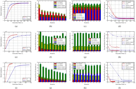
On the “clueweb” dataset, the execution times after 200 iterations were similar between both implementations, and they achieved similar model likelihood (see Fig. 6a). Both implementations are around 2.7 times faster than the results in data parallelism on the same dataset (see Fig. 5a) because sampling by words leads to less lock contention on the shared local model, and the routing in model rotation has less network conflicts than local/global model synchronization. The first 10 iterations show that “rtt” has high computation time compared with Petuum (see Fig. 6b). However, the additional overhead per iteration caused by communication becomes lower than Petuum. When the execution arrives at the final 10 iterations, while computation time per iteration in “rtt” is still higher, the whole execution time per iteration is now lower (see Fig. 6c). The trend of the iteration execution time on 200 iterations is shown in Fig 6d.
Unlike our “rotateGlobal” operation which batches trans-mission of model data partitions, Petuum sends model data word by word asynchronously, causing high communication overhead. On the “bi-gram” dataset, the results show that Petuum cannot perform well when the number of words in the model increases. The high overhead in communication causes the convergence speed to be very slow, and Petuum cannot even continue executing after 60 iterations due to a memory outage (see Fig. 6e). Fig. 6f and Fig. 6g show that in the first/final 10 iterations, Petuum consistently has higher execution time per iteration compared with “rtt”. The trend of the iteration execution time on 200 iterations also shows this phenomenon (see Fig. 6h).
Though the data size of “gutenburg” is similar to “enwiki”, it is clear that there is a difference in execution speed per iter-ation (see Fig. 6i). High standard deviiter-ation indicates that the iteration execution time per worker varies significantly. Unlike the results on “bi-gram” where Petuum’s performance suffers from the communication overhead, here it suffers from waiting for the slowest worker. The high iteration execution time may be explained by “gutenburg” containing many long documents and thereby resulting in unbalanced training data distribution on the workers. In addition, when sampling by words, frequent access to the shared huge doc-topic model leads to inefficient concurrent sampling. “rtt” is not much affected because it prefers using thread-local data in concurrent sampling and balances per-thread computation through assigning words to threads based on the frequencies. Fig. 6j, Fig. 6k, and Fig. 6l display that the unbalanced computation in Petuum results in high overhead per iteration. In model parallelism, model rotation is a synchronized operation; therefore, this experiment demonstrates that unbalanced computation on workers causes huge overhead in global waiting and results in high iteration execution time. In sum, when applying synchronized
commu-TABLE III
LDA WORKUSINGCGS ALGORITHM
App. Name Algorithm Parallelism Comm.
PLDA CGS (sample by docs) D. P. allreduce(sync)
Dato CGS (sample by doc-word edge) D. P. GAS(sync)
Yahoo! LDA CGS (SparseLDA &sample by docs) D. P. client-server
(async)
Peacock CGS (SparseLDA &sample by words) D. P. (M. P. inlocal) client-server
(async) Parameter
Server CGS (combined withother methods) D. P.
client-server (async)
Petuum 0.93 CGS (SparseLDA &sample by docs) D. P. client-server
(async)
Petuum 1.1 CGS (SparseLDA &sample by words) M. P. (includeD. P.) ring/startopology
(async) Note: “D. P.” refers to Data Parallelism. “M. P.” refers to Model Parallelism.
nication methods, the computation load should be carefully balanced.
VI. RELATEDWORK
Prior research has studied LDA algorithm parallelization extensively. Some studies focused on using the Collapsed Variational Bayes (CVB) algorithm [1], which is adapted by both Mahout LDA [17] and Spark LDA [18]. However, research also showed that this approach leads to high memory consumption and slow convergence speed [6][19].
Other studies used the CGS algorithm (see Table III). PLDA [20] is an implementation of this algorithm. Two versions of PLDA exist, one based on MPI [21] using “allreduce” operation [11] and the other based on MapReduce[10][22] using “shuffle” operation.
Yahoo! LDA [23][24] uses the CGS algorithm with SparseLDA optimization and client-server architecture. Local models are distributed in the star model and accessed with optimized locking mechanisms. The model synchronization is done through asynchronous delta aggregation.
Dato [25] uses the GAS model [26] to implement the LDA algorithm [27]. Currently, it uses a CGS algorithm without SparseLDA optimization. GAS model’s edge-based computation pattern causes the training data to be partitioned based on document-word pairs instead of documents. During the sampling process, the topic counts of both words and documents have to be gathered and updated, resulting in additional communication costs in synchronization.
0 5000 10000 15000 20000 25000
Execution Time (s)
−1.4
−1.3
−1.2
−1.1
−1.0
−0.9
−0.8
−0.7
−0.6
−0.5
Model
Lik
elihood
×1011
lgs-opt Yahoo!LDA lgs-opt-4s
(a)
0 5000 10000 15000 20000 25000
Execution Time (s)
0 100 200 300 400 500 600 700 800 Ex ecutionT ime Per Iteration
(s) lgs-opt-iterYahoo!LDA-iter lgs-opt-4s-iter
(b)
0 50 100 150 200
Num. of Synchronization Passes
0 100 200 300 400 500 600 700 800 Ex ecutionT ime Per SyncP ass (s) lgs-opt-comm Yahoo!LDA-comm lgs-comm (c)
0 50 100 150 200
Num. of Synchronization Passes
0 100 200 300 400 500 600 700 800 Ex ecutionT ime Per SyncP ass (s) lgs-opt-comm Yahoo!LDA-comm lgs-comm (d)
0 500 1000 1500 2000 2500 3000 3500
Execution Time (s)
−1.3
−1.2
−1.1
−1.0
−0.9
−0.8
−0.7
−0.6
−0.5
Model
Lik
elihood
×1010
lgs-opt Yahoo!LDA
(e)
0 500 1000 1500 2000 2500 3000 3500
Execution Time (s)
0 10 20 30 40 50 60 70 80 Ex ecutionT ime Per Iteration
(s) lgs-opt-iterYahoo!LDA-iter
(f)
0 50 100 150 200
Num. of Synchronization Passes
0 20 40 60 80 100 120 140 160 Ex ecutionT ime Per SyncP ass (s) lgs-opt-comm Yahoo!LDA-comm lgs-comm (g)
0 50 100 150 200
Num. of Synchronization Passes
[image:9.612.69.542.71.274.2]0 20 40 60 80 100 120 140 160 Ex ecutionT ime Per SyncP ass (s) lgs-opt-comm Yahoo!LDA-comm lgs-comm (h)
Fig. 5. Performance comparison on data parallelism between “lgs” and Yahoo! LDA (a) Elapsed Execution Time vs. Model Likelihood on “clueweb” (b) Elapsed Execution Time vs. Iteration Execution Time on “clueweb” (c) Num. of Sync. Passes vs. Sync. Time per Pass on “clueweb” with ib (d) Num. of Sync. Passes vs. Sync. Time per Pass on “clueweb” with eth (e) Elapsed Execution Time vs. Model Likelihood on “enwiki” (f) Elapsed Execution Time vs. Iteration Execution Time on “enwiki” (g) Num. of Sync. Passes vs. Sync. Time per Pass on “enwiki” with ib (h) Num. of Sync. Passes vs. Sync. Time per Pass on “enwiki” with eth
0 1000 2000 3000 4000 5000 6000 7000 8000
Execution Time (s)
−1.4
−1.3
−1.2
−1.1
−1.0
−0.9
−0.8
−0.7
−0.6
−0.5
Model
Lik
elihood
×1011
rtt Petuum
(a)
1 2 3 4 5 6 7 8 9 10
Iteration 0 50 100 150 200 250 300 Ex ecutionT ime Per Iteration (s) 181 131
121 116 112 106
100 92 85 80 57
23 21 18 19
18 17 18
16 15
59 54 52 50 48 44 42 39 36 35 33
30 28 32 29 29 31 29 30 26
rtt-compute rtt-overhead Petuum-compute Petuum-overhead
(b)
191 192 193 194 195 196 197 198 199 200
Iteration 0 5 10 15 20 25 30 35 Ex ecutionT ime Per Iteration (s)
23 23 23 23 23 23 23 23 23 23 3 3 3 2 3 3 3 2 3 3
19 19 19 19 19 19 19 19 19 19 10 10 10 11 9 10 9 9 10 10
rtt-compute rtt-overhead Petuum-compute Petuum-overhead
(c)
0 1000 2000 3000 4000 5000 6000 7000
Execution Time (s)
0 50 100 150 200 250 Ex ecutionT ime Per Iteration
(s) rtt-computertt-iter Petuum-compute Petuum-iter
(d)
0 1000 2000 3000 4000 5000 6000
Execution Time (s)
−2.4
−2.3
−2.2
−2.1
−2.0
−1.9
−1.8
−1.7
Model
Lik
elihood
×1010
rtt Petuum
(e)
1 2 3 4 5 6 7 8 9 10
Iteration 0 20 40 60 80 100 120 Ex ecutionT ime Per Iteration (s) 28 16
12 11 10 9 8 7 7 6 71
38
31 29
36 36
27 25 25 25
7 7 7 7 6 6 6 6 6 6 110
87 84
82 81 86 86 85 102 84 rtt-compute rtt-overhead Petuum-compute Petuum-overhead (f)
53 54 55 56 57 58 59 60 61 62
Iteration 0 20 40 60 80 100 Ex ecutionT ime Per Iteration (s)
4 4 4 4 4 4 4 4 4 4 19 20 21 21 19 19 19 19 19 20
6 6 6 6 6 6 6 6 6 6 82 86 86 84 86
81 86 87 83 88 rtt-compute rtt-overhead Petuum-compute Petuum-overhead (g)
0 1000 2000 3000 4000 5000 6000
Execution Time (s)
0 20 40 60 80 100 120 Ex ecutionT ime Per Iteration (s) rtt-compute rtt-iter Petuum-compute Petuum-iter (h)
0 500 1000 1500 2000 2500
Execution Time (s)
−8.0
−7.5
−7.0
−6.5
−6.0
−5.5
Model
Lik
elihood
×109
rtt Petuum
(i)
1 2 3 4 5 6 7 8 9 10
Iteration 0 20 40 60 80 100 120 140 Ex ecutionT ime Per Iteration (s) 36 24 20
16 14 12 10 8 7 5 15
9 8
8 8 8 8 7 7 7 19 17 15 14 12 11 10 9 8 8 108 90 85 73 75 65 61 57 54 49 rtt-compute rtt-overhead Petuum-compute Petuum-overhead (j)
91 92 93 94 95 96 97 98 99 100
Iteration 0 2 4 6 8 10 12 14 Ex ecutionT ime Per Iteration (s)
1 1 1 1 1 1 1 1 1 1 3 3 3
3 3 3 3 3 3 3 6 6 6 6 6 6 5
5 6 6 5 5
5 5 6 5 5 6 5 5
rtt-compute rtt-overhead Petuum-compute Petuum-overhead
(k)
0 500 1000 1500 2000 2500
Execution Time (s)
0 20 40 60 80 100 120 140 Ex ecutionT ime Per Iteration
(s) rtt-computertt-iter Petuum-compute Petuum-iter
(l)
[image:9.612.69.544.335.647.2]documents. The second layer uses client-server architecture with asynchronous communication.
Parameter Server [28] and Petuum [29] provide a framework in client-server architecture to allow users to program ma-chine learning algorithms with “push” and “pull” operations. Parameter Server puts the global model on servers and uses range-based “push” and “pull” operations for synchronization. These operations allow workers to update a row or segment of parameters directly and enables batching the communication of model updates. The computation of Parameter Server’s LDA implementation uses a combination of stochastic variational methods, collapsed Gibbs sampling, and distributed gradient descent. Another operation of Petuum, “schedule”, allows model parallelism through scheduling model partitions to workers. Lee et al. [30] describes that the communication to fetch model data goes between clients and servers, but in the real code on GitHub [4], workers are directly sending data to neighbors with optimized routing.
VII. CONCLUSION
Through experiments on several datasets, we showed that synchronized communication methods perform better than asynchronous methods on both data parallelism and model parallelism. In data parallelism, our implementation resulted in faster model convergence and higher model likelihood at iteration 200 compared to Yahoo! LDA using asynchronous communication methods. In model parallelism, our implemen-tation also showed significantly lower overhead than Petuum LDA. On “bi-gram” dataset, the total execution time of “rtt” is 3.9 times faster. Even though the computation speed of the first iteration is 2- to 3-fold slower on “clueweb” dataset, the total execution time remains similar. These results prove that with synchronized communication optimizations, we can increase the model update rate, which allows the model to converge faster, shrinks the model size, and reduces the computation time in later iterations.
Despite the implementation differences between “rtt”, “lgs”, Yahoo! LDA, and Petuum LDA, the advantages of synchro-nized communication methods can be understood. Compared with asynchronous communication methods, synchronized communication methods can optimize routing between a set of parallel workers and maximize bandwidth utilization in point-to-point communication. Though synchronized commu-nication methods will result in global/local waiting, balancing the computation on all parallel workers is feasible since the word frequencies in the LDA training data are under the power-law distribution and a considerable amount of words have high frequencies. Thus, the overhead of waiting is not as high as speculated. The chain reaction set off by improving the LDA model update speed amplifies the benefit of using synchronized communication methods.
In future work, we will focus on improving intra-node model synchronization speed in many-core systems to provide a high performance LDA implementation, understanding the performance impact when applying data parallelism or model parallelism in LDA, and applying our model synchronization
strategies to other machine learning algorithms facing difficul-ties in synchronizing big model data.
ACKNOWLEDGMENT
We gratefully acknowledge support from Intel Parallel Com-puting Center (IPCC) Grant, NSF 1443054 CIF21 DIBBs 1443054 Grant, and NSF OCI 1149432 CAREER Grant. We appreciate the system support offered by FutureSystems.
REFERENCES
[1] D. M. Blei, A. Y. Ng, and M. I. Jordan, “Latent dirichlet allocation,”
The Journal of Machine Learning Research, vol. 3, pp. 993–102, 2003. [2] B. Zhang, Y. Ruan, and J. Qiu, “Harp: collective communication on
hadoop,” inIC2E, 2015.
[3] “Yahoo! LDA.” [Online]. Available: https://github.com/sudar/Yahoo LDA
[4] “Petuum LDA.” [Online]. Available: https://github.com/petuum/bosen/ wiki/Latent-Dirichlet-Allocation
[5] P. Resnik and E. Hardist, “Gibbs sampling for the uninitiated,” Univer-sity of Maryland, Tech. Rep., 2010.
[6] D. Newman et al., “Distributed algorithms for topic models,” The
Journal of Machine Learning Research, vol. 10, pp. 1801–1828, 2009.
[7] J. Yuan et al., “LightLDA: big topic models on modest computer
clusters,” inWWW, 2015, pp. 1351–1361.
[8] L. Yao, D. Mimno, and A. McCallum, “Efficient methods for topic
model inference on streaming document collections,” in KDD, 2009,
pp. 937–946.
[9] C.-T. Chuet al., “Map-reduce for machine learning on multicore,” in
NIPS, vol. 19, 2007, p. 281.
[10] J. Dean and S. Ghemawat, “MapReduce: simplified data processing on
large clusters,”Communications of the ACM, vol. 51, no. 1, pp. 107–113,
2008.
[11] E. Chanet al., “Collective communication: theory, practice, and
experi-ence,”Concurrency and Computation: Practice and Experience, vol. 19,
no. 13, pp. 1749–1783, 2007.
[12] “fastutil.” [Online]. Available: http://fastutil.di.unimi.it
[13] “FutureSystems.” [Online]. Available: https://portal.futuresystems.org [14] “wikipedia.” [Online]. Available: https://www.wikipedia.org
[15] “clueweb.” [Online]. Available: http://boston.lti.cs.cmu.edu/clueweb09/ wiki/tiki-index.php?page=Dataset+Information
[16] “gutenburg.” [Online]. Available: https://www.gutenberg.org
[17] “Mahout LDA.” [Online]. Available: https://mahout.apache.org/users/ clustering/latent-dirichlet-allocation.html
[18] “Spark LDA.” [Online]. Available: http://spark.apache.org/docs/latest/ mllib-clustering.html
[19] Y. Wanget al., “Peacock: learning long-tail topic features for industrial
applications,”ACM Transactions on Intelligent Systems and Technology,
vol. 6, no. 4, 2015.
[20] Y. Wanget al., “PLDA: parallel latent dirichlet allocation for large-scale
applications,”Algorithmic Aspects in Information and Management, pp.
301–314, 2009.
[21] D. W. Walker and J. J. Dongarra, “MPI: a standard message passing
interface,” inSupercomputer, vol. 12, 1996, pp. 56–68.
[22] “Hadoop.” [Online]. Available: http://hadoop.apache.org
[23] A. Smola and S. Narayanamurthy, “An architecture for parallel topic
models,” inVLDB, vol. 3, no. 1-2, 2010, pp. 703–710.
[24] A. Ahmed et al., “Scalable inference in latent variable models,” in
WSDM, 2012, pp. 123–132.
[25] “Dato.” [Online]. Available: https://dato.com
[26] J. E. Gonzalezet al., “PowerGraph: distributed graph-parallel
computa-tion on natural graphs,” inOSDI, vol. 12, 2012, p. 2.
[27] “Dato LDA.” [Online]. Available: https://github.com/dato-code/ PowerGraph/blob/master/toolkits/topic modeling/topic modeling.dox
[28] M. Liet al., “Scaling distributed machine learning with the parameter
server,” inOSDI, 2014, pp. 583–598.
[29] E. P. Xing et al., “Petuum: a new platform for distributed machine
learning on big data,” inKDD, 2013.
[30] S. Leeet al., “On model parallelization and scheduling strategies for