Abstract: Remote sensing is an important issue in satellite image classification. In developing a significant sustainable system in agriculture farming, the major concern for remote sensing applications is the crop classification mechanism. The other important application in remote sensing is urban classification which gives the information about houses, roads, buildings, vegetation etc. A superior indicator for the presence of vegetation can be computed from the vegetation indices of a satellite image. This indicator supports in describing the health of vegetation through the image attributes like greenness and density. The other parameter in detecting objects or region of interest is an image is the texture. A satellite image contains spectral information and can be represented by more spectral bands and classification is very tough task. Generally, Classification of individual pixels in satellite images is based on the spectral information. In this research paper Principle component analysis and combination of PCA and NDVI classification methods are applied on Landsat-8 images. These images are acquired from USGS. The performance of these methods is compared in statistical parameters such as Kappa coefficient, overall accuracy, user’s accuracy, precision accuracy and F1 accuracy. In this work existing method is PCA and proposed method is PCA+NDVI. Experimental results shows that the proposed method has better statistical values compared to existing method.
Keywords: Classification, Kappa coefficient, Multispectral images, NDVI, PCA.
I. INTRODUCTION
Remote sensing is the art of science obtaining and analyzing information about phenomenon, area or object using a physical device without a physical contact. It provides constant and tedious view of the earth surface [1]. It offers a reliable and repetitive perspective of the earth’s surface. Satellite imagery classification plays a significant role in many remote sensing applications. It is a technique by which, based on their spectral features, labels or class identifiers are connected to the pixels that making up remotely sensed images. These features are usually spectral reaction measurements in various wavebands. They also contain other attributes like vegetation. Remote sensing spectral vegetation indicators have been commonly used to assess and analyze biomass, water, and plants. Vegetation indices (VI) enhance spectral information and increase interest class separability, thus influencing the quality of information obtained from remote sensed data. Analysis of remotely sensed data can be
Revised Manuscript Received on August 20, 2019.
M Venkata Dasu*, Research Scholar, Dept of ECE, JNTUA, Anantapuramu, Andhra Pradesh.. Email: [email protected].
Dr P V N Reddy, Principal, Sri Venkateswara College of Engineering, Balaji Nagar, Kadapa, Andhra Pradesh – 516003, Email: [email protected].
Dr S Chandra Mohan Reddy, Associate Professor, Dept of ECE JNTUA, Anantapuramu, Andhra Pradesh. Email: [email protected].
distinguished by three factors [2-3].They are 1.Remote sensed images give a panoramic overview 2.Remote sensing images use the electromagnetic spectrum’s
visible and infra red regions.
3.They can describe the earth’s surface at different resolutions.
Remote sensing images may contain spectral and spatial information of the objects. Object classification is performed through the spectral analysis of the reflected or emitted by radiant energy of the target [4].In this paper a dynamic approach is used for the classification of satellite image. The paper is organized as follows section II describes the methodology of the research work and section III presents the experimental results and discussions .Conclusion of the research work is outlined in section IV.
II. PROPOSEDMETHODOLOGY
[image:1.595.304.552.523.667.2]A. Data Set: In this work Kalahasti area from Chittoor district in Andhra Pradesh is used for image classification. The satellite images are acquired from United States geological survey (USGS). The collected images are LANDSAT 8 OLI (operational Land imagery).Table 1 gives the characteristics of LANDSAT 8 OLI. In this work band 4 and band 5 are used for classification and they provide good accuracy when compared to other spectral bands. Region of interest (ROI) extracted from 143/50 row path. In this work ROI is Kalahasti. To extract desired area raster clip and shape file is applied on the satellite image.
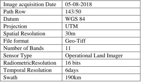
Table 1.Landsat 8 OLI characteristics Image acquisition Date 05-08-2018
Path Row 143/50
Datum WGS 84
Projection UTM
Spatial Resolution 30m
File format Geo-Tiff
Number of Bands 11
Sensor Type Operational Land Imager
RadiometricResolution 16 bits Temporal Resolution 6days
Swath 190km
The band designations of Landsat 8 are shown in Table 2.
Classification of Landsat-8 Imagery Based On
Pca And Ndvi Methods
Table 2.Landsat 8 Band Description
Bands Wavelength
(µm)
Resolution (m)
Band 1 0.43-0.45 30
Band 2 0.45-0.51 30
Band 3 0.53-0.59 30
Band 4 0.64-0.67 30
Band 5 0.85-0.88 30
Band 6 1.57-1.65 30
Band 7 2.11-2.29 30
Band 8 0.50-0.68 15
Band 9 1.36-1.38 30
Band 10 10.6-11.19 100
Band 11 11.5-12.51 100
Operational Line imager (OLI) and Thermal Infrared Sensor (TIRS) provides information in multispectral bands. A Landsat 8 OLI and TIRS satellite images contains 9 spectral bands .Band 1 to 7 has the spatial resolution of 30meters. Band1 is ultra blue used for the stud of coastal and aerosol. Band 2desribes Blue, Band 3 is Green, Band 4 is Red, Band 5 is Infra Red, Band 6 is Short Wave Infra Red (SWIR1), band 7 is Short Wave Infra Red 2(SWIR2), Band 8 is panchromatic and resolution of this band is 15 meters. Band 9 is useful for the identification of cirrus cloud detection [5-6]. A thermal band 10, 11 provides the accurate surface temperature and is collected at 100 meters.
[image:2.595.48.248.389.635.2]
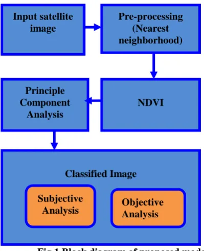
Fig.1 Block diagram of proposed model The proposed model contains four steps
Satellite image acquisition. Pre-processing.
Classification.
Error matrix calculation.
B. Image Acquisition:
The input satellite image for the proposed model is acquired from the united state geological survey (USGS). The collected images are LANDSAT 8 OLI (operational Land imagery).
C. Pre-Processing:
Next step in the proposed methodology is image preprocessing by nearest neighbor interpolation. The acquired image may contain noise and this can be removed and enhanced by nearest neighbor interpolation algorithm. From computational point of view nearest neighbor interpolation is simple and faster than the other interpolation techniques like linear interpolation, Bilinear and Bicubic interpolation techniques. In this algorithm for each pixel, intensity value is assigned by the nearest neighbor of the point in the input image. This procedure is known as replication. In this algorithm intensity value of f(x, y) is assigned to output image g(x, y).
D. NDVI:
In satellite image to measure the greenness of plants, commonly used indicator is vegetation index [7] .There are many vegetation indices are available but most often used index is the Normalized vegetation index (NDVI). The coverage of vegetation on the surface of the earth can be identified by examining the images from visible red and near-infrared wavelengths. It can be expressed as
NDVI=
RED
NIR
RED
NIR
…………. (1)
E. Principle Component analysis:
Principal Component analysis (PCA) is a statistical method used to decrease a set of correlated multivariate measure to a narrower set where the characteristics are uncorrelated. The emergence of satellite remote sensing in digital format with multispectral and hyper spectral images has introduced a fresh dimension to the stock, mapping and tracking of the earth’s natural recourses. The multi spectral (multiband) images were obtained various areas of the electromagnetic spectrum, thereby maintaining band correlation.PCA method have been integrated in the digital image processing of satellite images as a unique conversion in which a number of correlated image information bands have been reduced to few uncorrelated bands [8-10].
Multi-temporal and multiband images are needed to perform the PCA. The images input must share the same size (rows and columns), pre-processing level, amount of bands for each scene, geographic expansion, format, and preferably the same incident angle. The purpose of using PCA is to reduce the dimensionality of the data in order to maximize the amount of information from the original bands into the smallest number of PCs, the number of original bands in this case. A set of correlated variables (Original bands) is converted into other uncorrelated variables containing the highest initial data that requires being explored [11-14]. Assuming that a Multi-temporal image with eight input bands can be expressed in matrix format as follows.
Input satellite image
Pre-processing (Nearest neighborhood)
NDVI Principle
Component Analysis
Classified Image
Subjective
Xp,q=
q b q p px
x
x
x
x
x
, 1 , , 2 1 , 2 , 1 1 , 1...
.
.
...
...
……….(2)Here p represents number of pixels and b is the number of bands.The above matrix can be simplified as follows, consid ering each group as a vector [15-17]:
xk=
qx
x
x
.
.
2 1 ………(3)Where k is the band number. The covariance matrix’s Eigen values must be calculated to decrease the dimensionality of the original bands and covariance matrix can be calculated as follows
Cq,q=
q q q q , , 1 , 1 1 , 1...
.
.
...
……….(4)Where σx,y is the covariance of the different bands of each pair.
The Eigen values of covariance matrix can be calculated as the roots of the characteristic equation
det(C-λI)=0………..(5)
The matrix of the Principle component can be described from
Y8=
q q b qw
w
w
w
, 1 , , 1 1 , 1...
.
.
...
qx
x
x
.
.
2 1 …….(6)Where Y is the principal component vector, the transformati on matrix is w and the original data vector is x.
III. RESULTSANDDISCUSSIONS
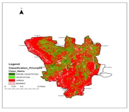
In this work satellite image which acquired with Landsat 8 is classified by combining NDVI and Principle component analysis in order to improve the classification accuracy. The results are compared with the PCA alone. The acquired image is Kalahasti area, Andhrapradesh. India. This image is analyses with remote sensing software called ArcGIS 10.3 used. The Size of the acquired image is 7631×7801 and the Region of interest is Kalahasti and is extracted from 143/50 (row/path).
Fig.2. Satellite image classification with PCA The classified image contains four classes i.e., dense vegetation, Vegetation, urban and barren land. Figure 2 shows the classified satellite image using NDVI and PCA. The error matrices for the two images were calculated and the performance of these methods is statistically compared.
Fig.3. Satellite image classification with NDVI and PCA
The accuracy of the classification methods can be obtained by error matrix. The error matrices for PCA and NDVI+PCA shown in below.Tables.
Table 3.Error matrix for PCA Land
cover
Dense vegetation
Vegetation Urban Ba
rren Land Dense
vegetati on
29 1 0 1
Vegetat ion
0 28 1 1
Urban 1 0 27 0
Barren Land
1 0 0 29
Row Total
Table 4.Error matrix for PCA+NDVI Land
cover
Dense vegetation
Vegetation Urban Barren
Land Dense
vegetation
30 0 0 1
Vegetatio n
1 29 0 0
Urban 0 1 29 0
Barren Land
1 0 0 28
Row Total 32 30 28 30
[image:4.595.52.291.416.562.2]Table 2 and Table 3 shows the error matrix or confusion matrix for existing (PCA) and proposed (PCA+NDVI) methods. As a quantitative method of characterizing image classification precision, a confusion matrix (or error matrix) is generally used. It is a table showing correspondence between the consequence of the classification and the reference image I.e., to generate a confusion matrix, ground-truth data such as cartographic information, manual image digitization outcomes, field work / ground survey findings are required. In error matrix table cells indicates the amount of correlation between ground truth image and classified image. Diagonal elements in the matrix give the correctly identified pixels. from several accuracy indicating parameters are calculated from the error matrix.
Table 5.Performance Analysis
S.No Parameters PCA PCA+NDVI
1 Users
Accuracy
0.94 0.96
2 Producer
Accuracy
0.95 0.95
3 Overall
Accuracy
0.94 0.96
4 Kappa
coefficient
0.93 0.95
5 F1 Score 0.95 0.96
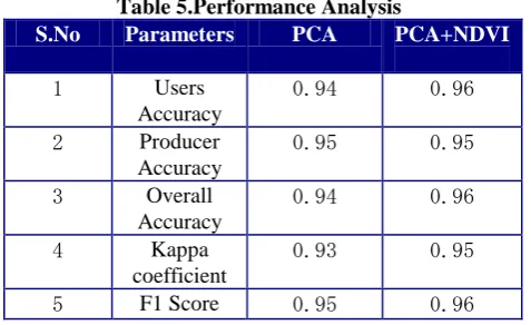
The parameters are listed in a table 5. The parameters considered in this work is various performance metrics like user’s accuracy, producer’s accuracy, overall accuracy Kappa coefficient and F1 score are listed in the table5.
Kappa coefficient is the important parameter and it can a value between 0 to 1.if kappa coefficient is 1classified image ground truth data are same. If more the kappa coefficient, the classification accuracy is high.
Fig.4. Graphical representation of statistical parameters.
From the Table 5 the proposed method has better values than the existing method and the figure 4 shows the graphical representation of the parameters.
IV. CONCLUSION
Satellite image classification plays an important role in providing the geographical information. It provides the quantitative and qualitative information that reduces field work and stud complexity. In this work NDVI is combined with the PCA and the results are compared with the PCA. The experimental results are better for proposed method than existing method.
ACKONOWLEDGEMENT
The first author is a research scholar in Jawaharlal Nehru Technological University Anantapur, Anantapuramu and expresses his sincere thanks to JNTUA, AITS, Rajampeta and USGS (Landsat-8) for providing research facilities.
REFERENCES
1. D.Jeeva lakshmi, S.Naraana Reddy,” Land Cover Classification based on NDVI using LANDSAT8 Time Series: A Case Study Tirupati Region”, in International Conference on Communication and Signal Processing, April 6-8, 2016,pp.1332-1335.
2. Malgorzata VER_NE WOJTASZEK, Aniko KLUJBER, Erzsebet VECSEI, “Comparison of Different Image Classification Methods in Urban Environment,” International Scientific Conference on Sustainable Development & Ecological Footprint, March, 2012 Sopron, Hungary.
3. Bhandari AK, Kumar A, Singh G.K, “Feature Extraction using Normalized Difference Vegetation Index (NDVI): a Case Study of Jabalpur City,” Procedia Technology, 6, pp.612-621.
4. Meera Gandhi.G, S.Parthiban, Nagaraj Thummalu and Christy. A, “Ndvi: Vegetation change detection using remote sensing and GIS – A case study of Vellore District,” 3rd International Conference on Recent Trends in Computing 2015 (ICRTC-2015), ScienceDirect, Procedia Computer Science 57 (2015) 1199 – 1210
5. Liu, L.; Zhang, Y. “Urban Heat Island Analysis Using The Landsat TM Data And Aster Data: A Case Study In Hong Kong,” Remote Sens. 2011, 3, 1535-1552; doi:10.3390/rs3071535. Ndvi
6. Kun Jia , Shunlin Liang , Xiangqin Wei, Yunjun Yao, Yingru Su, Bo Jiang and Xiaoxia Wang, “Land Cover Classification of Landsat Data with Phenological Features Extracted from Time Series MODIS NDVI Data,” Remote Sensing, 6(11): 11518–11532. doi: 10.3390/rs61111518.
7. Ardavan Ghorbani, Amir Mirzaei Mossivand and Abazar Esmali
Ouri, land/canopy cover mapping in Khalkhal County (Iran),”
Scholars Research “Utility of the Normalised Difference
Vegetation Index (NDVI) for Library, Annals of Biological
Research, 2012, 3 (12):5494-5503.
8. David Gómez-Palacios,” Flood mapping through principal component analysis of multitemporal satellite imagery considering the alteration of water spectral properties due to turbidity conditions”,In Geomatics, Natural Hazards And Risk, 2017, Vol. 8, No. 2, 607–623.
9. Estornell J, Mart_ı-Gavil_a M, Sebasti_a MT, Mengual J. 2013. Principal component analysis applied to remote sensing. MSEL. 6:83–89.
10. Fraser SJ. 1991. Discrimination and identification of ferric oxides using satellite thematic mapper data: a Newman case study. Int J Remote Sens. 12:635–641.
11. Dhaka of Bangladesh using remote sensing and GIS techniques. Water Resour Manag. 21:1601–1612. Estornell J, Mart_ı-Gavil_a M, Sebasti_a MT, Mengual J. 2013. Principal component analysis applied to remote sensing. MSEL.
[image:4.595.54.269.686.787.2]12. Dai X, Khorram S. 1998. The effects of image misregistration on the accuracy of the remotely sensed change detection. IEEE Trans Geosci Remote Sen. 36:1566–1577.
13. Green AA, Berman M, Switzer P, Craig MD. 1988. A transform for ordering multispectral data in terms of image quality with implications for noise removal. IEEE Trans Geosci Remote Sens. 26:65–74 14. Gupta RP, Tiwari RK, Saini V, Srivastava N. 2013. A simplified
approach for interpreting principal component images. Adv Remote Sens. 2:111–119.
15. Ingebritsen SE, Lyon RJP. 1985. Principal components analysis of multitemporal image pairs. Int J Remote Sens. 6:687–696.
16. Jain SK, Singh RD, Jain MK, Lohani AK. 2005. Delineation of flood-prone areas using remote sensing techniques. Water Resour Manag. 19:333–347.