promoting access to White Rose research papers
Universities of Leeds, Sheffield and York
http://eprints.whiterose.ac.uk/
White Rose Research Online URL for this paper:
Conference paper
Ibrahim, SS, Gubba, SR and Malalasekera, W (2010) A Parametric Study on
Large Eddy Simulations of Turbulent Premixed Flames. In: Mishra, DP and
A Parametric Study on Large Eddy Simulations of
Turbulent Premixed Flames
Salah S Ibrahim
1, Sreenivasa Rao Gubba
2,*, Weeratunge Malalasekera
31, 3Faculty of Engineering, Loughborough University, Loughborough, LE11 3TU, UK
2CFD centre, School of Process, Environment and Materials Engineering, University of Leeds, Leeds, LS2 9JT, UK
Abstract:A parametric study has been carried out on the use of large eddy simulations (LES) technique for the prediction of turbulent premixed flames. A flame surface density (FSD) model is used together with an algebraic closure to calculate the filtered reaction rate. This reaction rate needs to be appropriately modelled. One main objective of the present study is to evaluate and validate the model used against measured data obtained from laboratory scale experiments. In particular, the model performance is examined by varying controlling parameters such as ignition radius, model constant, filter width and test to grid filter ratio. Flame structure, speed and generated overpressure are used for model evaluations at
different times following ignition. The experimental
combustion chamber is 0.625 litres in volume with three built-in solid obstacles. The mixture used is a stoichiometric propane/air mixture with equivalence ratio 1.0. The results show sensitivity of the model to the specification of the initial ignition radius and grid resolution. However, the model is found to be less sensitive to the selected filter width.
Keywords: LES; premixed flames; turbulence; flame surface
density.
1. INTRODUCTION
With ever growing demand for eco-friendly, optimised combustion systems, fundamental understanding of the combustion phenomena is vital. Supported by continuous development in computational power and resources, numerical modelling such as large eddy simulations (LES) provides a potential alternative to expensive and difficult experimental investigations. In LES, large eddies above a certain cut-off length scale, generally known as filter width, are resolved and the smaller scales are modelled employing sub-grid scale (SGS) models. Recent work in this field [1-5] has confirmed the high fidelity of LES in predicting key characteristics of premixed flames. However, one essential requirement for the maturity of LES as a reliable numerical tool is, the need to establish methodologies for obtaining solutions that are independent of the size of the grid resolution and filter width.
Currently most formulations link the filter size to the numerical grid and these are referred to as implicit methods. The sub-grid filter must also be sufficiently fine to resolve a significant proportion of the turbulent kinetic energy [6]. Sensitivity of the LES results to modelling parameters related to SGS models, such as chemical reaction rate, is predominant and must also be understood. In addition, the modelling of the quasi-laminar phase of the initial stages of turbulent flames is very sensitive to ignition radius and initial conditions. These must be understood prior to their application.
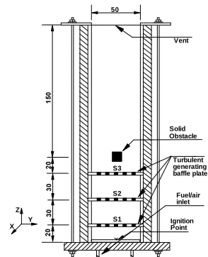
This paper examines and validates various important controlling parameters for LES simulations of turbulent premixed propane/air flames at an equivalence ratio of 1.0, which has practical importance in investigating explosion hazards and gas turbine combustors. The experimental test case chosen is constructed at the University of Sydney [7 & 8] and shown in Fig.1. The published experimental data [] for the flame structure and generated overpressure are used for examination and analysis. The chamber has a square cross section of 50mm and a height of 250mm, resulting in a total volume of 0.625l. Three baffle plates and a square obstacle are placed at different downstream location from the bottom ignition end. Each baffle plate has a 50×50mm aluminium frame constructed from 3mm thick sheeting, on which are mounted five 4mm wide bars each with a 5mm separation between them rendering a blockage ratio of 40%. The square solid obstacle is of 12×12mm cross section running across the chamber. The baffle plates are aligned at 90 degrees to the solid obstacle in the configuration employed in the present study. More details of the chamber can be found in earlier publications [3 & 4].
2. THELES MODEL
In applying LES to turbulent premixed flames, there are two basic requirements for SGS modelling of scalar fluxes and chemical reaction. The standard Smagorinsky [9] model developed in 1963 has been widely used to model the sub-grid fluctuations in the velocity field. Germano, Piomeli, Moin and
S1 S2 S3
Obstacle 50
Solid Vent
Ignition Point
Turbulent generating baffle plates
Fuel/air inlet
Y Z
[image:3.595.88.235.93.274.2]X
Fig. 1 Schematic diagram of the premixed combustion chamber. All dimensions are in mm
Cabot [10] extended this model by devising an automated procedure for determining the Smagorinsky model coefficient. In the present simulations the model coefficient is calculated from the instantaneous flow conditions using the dynamic determination procedure developed by Moin, Squires, Cabot and Lee [11] for compressible flows. The chemical reaction is modelled based on the flame surface density (FSD), , which is derived as flame surface area per unit volume. The mean reaction rate per unit volume, is determined from:
R
Here R is a mean reaction per unit surface area and is either modelled [12] or obtained by solving a full transport equation for the FSD [13]. Mean reaction rate per unit surface area R can be written as uuL, where uis unburned mixture density
anduLis laminar flame velocity. Following the DNS analysis of thin premixed flames Boger, Veynante, Boughanem and Trouve [14] deduced an algebraic expression for as:
) ~ 1 ( ~
4 c c
where c~ is the Favre filtered reaction progress variable, is the filter width and is a model constant referred to as Bogers
constant throughout this paper. This approach is implemented
in present simulations and Bogers constant, is varied as 1.2, 1.4 and 1.8. The above expression is similar to the Bray-Moss-Libby (BML) expression for FSD in RANS [15] with the ratio
/ representing the degree of sub-grid scale flame
wrinkling.
3.NUMERICAL METHODOLOGY
An in-house LES code called PUFFIN [16] is used to simulate propagation of the propane/air flame over solid obstacles. The initial condition of the mixture is stagnant prior to ignition. The LES code solves fully compressible, strongly coupled, Favre-filtered flow equations discretised using a finite volume method described in our earlier publications [3 & 17]. The discretisation is based on control volume formulation on a staggered non-uniform Cartesian grid. The filter width is calculated using a box filter [3, 16 & 17], which is related to grid resolution in general and fits in with the finite volume
discretisation. A second order central difference
approximation is used for diffusion, advection and pressure gradient terms in the momentum equations and for gradient in the pressure correction equation. Conservation equations for scalars use a second order central difference scheme for diffusion terms. Third order upwind schemes QUICK and SHARP are used for advection terms of the scalar equations to avoid problems associated with oscillations in the solution. The QUICK scheme is also sometimes used for the momentum equations in areas of the domain where the grid is expanded and accurate calculation of the flow is less important. The equations are advanced in time using the fractional step method. The Crank-Nicolson scheme is used for the time integration of momentum and scalar equations. A number of iterations are required at every time step due to the strong coupling of solved equations.
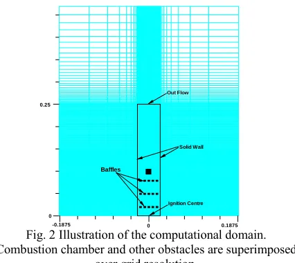
The computational domain together with boundary conditions is shown in Fig. 2. The combustion chamber has dimensions of 50×50×250mm where the flame propagates over the baffles and solid obstacle. Solid boundary conditions are applied at the bottom, vertical walls, for baffles and the obstacle by setting the normal and tangential velocity components to zero. This ideally represents impermeable and no-slip conditions. The walls and obstacles are considered to be isothermal and the same temperature is maintained thorough out the simulations. The wall shear is calculated by the 1/7th
sensitivity of the ignition radius and initial value of reaction progress variable within the radius are studied and presented here to achieve the initial quasi-laminar phase corresponding to experiments.
The governing equations, discretised by the finite volume method, are solved using a Bi-Conjugate Gradient solver with an MSI pre-conditioner for the momentum, scalar and pressure correction equations. The time step is limited to ensure the CFL number remains less than 0.5 with the extra condition that the upper limit for
t
is 0.3ms. The solution for each time step requires around 8 iterations to converge, with residuals for the momentum equations less than 2.5×10⁻⁵andscalar equations less than 2.0×10⁻³. The mass conservation
error is less than 5.0×10⁻⁸.
4.RESULTS AND DISCUSSION
LES predictions of propagating turbulent premixed flames of propane/air mixture at an equivalence ratio of 1.0 in the combustion chamber, shown in Fig. 1, are presented here using the FSD model described in Section 2. Numerical predictions are compared with available averaged measurements, which include pressure-time traces, high speed video images of flame emissions, flame position and speed, that are derived from video images. A grid resolution of 90x90x336 (2.7 million cells) is adopted in the present calculations, as further refinement to 3.6 million cells shows no significant improvement in results for the present configuration [3]. One of the main objectives of this paper is to examine and assess the influence of various controlling parameters in LES.
4.1 Influence of Ignition Radius and Progress Variable
In numerical simulations of turbulent premixed flames it is important to mimic the quasi-laminar phase of the initial stage
of turbulent flame after ignition. The quasi-laminar phase is generally achieved by setting a reaction progress variable,c~
within certain ignition radius. In order to achieve stable and accurate LES predictions, it is important to understand the sensitivity of these parameters. Seven LES cases as detailed in Table 1 are carried out with four different ignition radii (3-6mm) and initial c~ values of 0.5 and 0.7. The influence of
test filter to grid filter ratio, also studied here by choosing two values i.e. 1.362 and 2.0 as detailed in Table 1. The basic idea of this analysis is to verify the appropriate ignition radius, in order to achieve the quasi-laminar phase of the premixed propagating flame. The peak overpressure and its incidence time are also detailed in Table 1.
Figs. 3 and 4 present the pressure-time histories obtained from LES simulations against experimental overpressure for cases A-D and E-G respectively. It is evident from Fig. 3 and Table 1 that the differences in peak overpressure magnitudes are not significant. However, the time of its occurrence is dependent upon the ignition radius. Comparing cases E and F in Fig. 4 confirms that increasing the initial value of c~ results
in reducing the magnitude of peak overpressure. A similar time shift of approximately 0.4 ms can be observed while using a 4mm ignition radius, with little impact on overpressure. It is very interesting to note that using burning (c~ = 0.5) to completely burned conditions (approaching c~ =
0.7 or higher) to initialise the ignition, dramatically shifts the timing. This type of tuning to achieve the correct timing of peak overpressure at a chosen ignition radius may be a good option and but it does not represent the ignition and after ignition processes correctly. It can also be identified that, irrespective of the radius chosen to initialise ignition,
overpressure predictions show a maximum of 12% variation,
which is quite encouraging in choosing the appropriate value of ignition radius to achieve the correct timing.
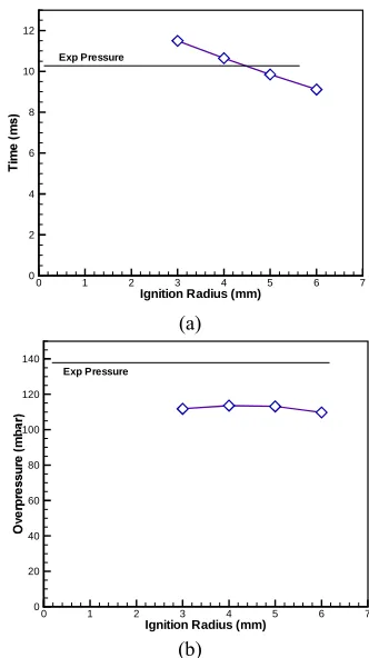
[image:4.595.72.285.83.273.2]Figs. 5a and 5b presents values of the time of occurrence of peak overpressure and its magnitude, respectively, for cases A-D. It is very interesting to note, from these figures, that the ignition radius of the hemispherical region has a linear relation
Table 1: Outcome of LES simulations using various ignition radii and initial reaction progress variable values
Case Ignition radius (mm) c
~ Peak
Overpressure (mbar)
Time of Occurrence
(ms)
A 3 0.5 1.362 111.8 11.5
B 4 0.5 1.362 113.6 10.6
C 5 0.5 1.362 113.2 9.90
D 6 0.5 1.362 109.7 9.10
E 4 0.7 1.362 112.8 11.0
F 6 0.7 1.362 110.0 9.70
G 4 0.5 2.0 124.6 11.0
Fig. 2 Illustration of the computational domain. Combustion chamber and other obstacles are superimposed
over grid resolution.
Solid Wall Out Flow
Ignition Centre
Baffles
0 0.1875 -0.1875
0.25
[image:4.595.301.543.592.696.2]with respect to peak overpressure incidence. The straight horizontal line in Fig. 5a represents the time of experimental peak overpressure, which corresponds approximately to an ignition radius of about 4.5mm. However, Fig. 5b confirms once again that the influence of ignition radius on overpressure is insignificant.
Snap-shots of the reaction rate contours from LES simulations of A-D at peak overpressure time are presented in Fig. 6. They confirm that irrespective of chosen ignition radius, the contours represent a similar propagating flame scenario in the combustion chamber. Fig. 6 shows very few differences, at this instance, in flame position, thickness, pockets, shape of recirculation zone and structure. It is quite encouraging that all LES simulations have predicted the overall flame characteristics very well.
Fig. 4 also presents the LES prediction (Case G) using = 2.0 with a reaction progress variable of 0.5 within a 4mm radius of ignition. This LES simulation is quite remarkable in achieving the closest peak overpressure i.e. 124.6 mbar with a small time shift of 0.68 ms from the experimental pressure
reference. Case G confirms that test filter to grid filter ratio ( ) has significant influence on overpressure predictions. The under-prediction of overpressure in cases A-F can be clearly attributed to the chosen value for . In addition to this analysis, it is identified in [19], from over a hundred experimental pressure measurements at base and wall in the same chamber, that this shifting is only recognized in a small number of experiments involving no more than 1-2ms, thus confirming that the present LES predictions are within the experimental tolerance. Hence, it can be confirmed that the LES predictions are sensitive to ignition radius, initial value of reaction progress variable and test to filter width ratio. It is also noticed that cases B, E and G having ignition radii of 4 mm are closest in mimicking the initial quasi-laminar phase corresponding to experiments as seen in videos and reaction rate movies (not shown here). This observation is also in agreement with the experimental observations of Bradley and Lung [20]. 4mm is chosen as the ignition radius for further LES simulations presented in next sections.
(a)
Fig. 5 (a) Peak overpressure incidence time for cases A-D (3-6mm) (b) Magnitude of the peak overpressure predicted
for cases A, B, C & D Ignition Radius (mm)
0 1 2 3 4 5 6 7
0 2 4 6 8 10 12
Exp Pressure
Ignition Radius (mm)
0 1 2 3 4 5 6 7
0 20 40 60 80 100 120 140
Exp Pressure
[image:5.595.81.247.82.220.2](b) Fig. 3 Overpressure time traces of LES simulations using
various ignition radiuses and reaction progress variable.
Time (ms)
0 2 4 6 8 10 12 14
0 50 100 150
4 mm, c=0.7 4 mm, c=0.5 , TF=2.0 6 mm, c=0.7 Exp
Fig. 4 Overpressure time traces of LES simulations using various ignition radiuses and reaction progress variable.
Time (ms)
0 2 4 6 8 10 12 14
0 50 100 150
[image:5.595.81.250.253.388.2] [image:5.595.343.509.331.627.2]4.2 Influence of Bogers Constant ( )
Bogers constant, as described in Section 2 plays a major role in controlling the mean chemical reaction rate and thus
influences flame dynamics. Three LES cases with Bogers
[image:6.595.78.271.81.217.2]constants of 1.2, 1.4 and 1.8 are considered here as detailed in Table 2. It is worth mentioning at this stage that the test filter to grid filter ratio ( ) is considered as 2.0 for all these cases. Table 2 also delineates LES predictions for these cases against experimental measurements.
Fig. 7 shows overpressure time histories of three cases (G-I) against measurements. Fig. 8 shows flame positions obtained from LES simulations against experimental flame positions that are derived from video images. It is quite interesting to note that as the value of increases, the overpressure trend in Fig. 7 is progressively increasing. It should also be noted that, with a higher value of the flame burns faster. This phenomenon is clearly confirmed by the
predicted flame positions in Fig. 8. As Bogers constant is
related to SGS flame wrinkling factor, an increase of this value is expected to increase the degree of flame wrinkling and thus increases the surface area of the reacting flame. As a result, the reaction zone thickness increases as it consumes more unburned mixture downstream of the chamber. It is also noticed that the flame front is becoming sensitive with to the resolved turbulent motions as seen in reaction rate movies (not shown here) from LES predictions.
Table 2: LES predictions using various values for Bogers
constant against experimental measurements.
Case
Bogers constant
( )
Time (ms)
Peak overpressure
(mbar)
Flame Position
(cm)
Flame Speed (m/s)
G 1.2 11.0 124.6 18.9 81.5
H 1.4 9.7 139.9 17.0 85.0
I 1.8 7.8 204.1 19.8
--Exp -- 10.3 138.0 15.0 56.0
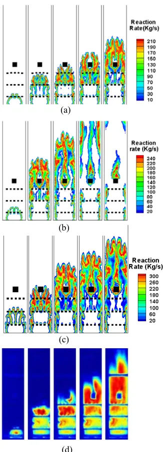
Fig. 9 shows a sequence of reaction rate contours for three LES cases and images from experimental high speed video recordings at various stages. Individual reaction rate contour legends for LES is also shown in Figs. 9a-9c. From these, it is evident that, as the value of is increased, the magnitude of reaction rate follows thus causing over-prediction of flame
characteristics. In Case H ( = 1.4) though the peak
overpressure is in agreement with experiments, it is clear that the flame is much faster and leaving the chamber at an early stage. In Case I ( = 1.8), LES is over-predicting the flame characteristics at an earlier stage than experiments. However, in Case G ( = 1.2), LES predictions are in reasonable agreement i.e. the peak overpressure is within 10% of experimental tolerance and with a correct flame position up to blowout phase. Hence, it is clear from these simulations that
the Bogers constant is one of the key parameters on which
flame is highly dependent or in other words; choosing a correct will provide better results. However, combining the results presented in Figs. 7, 8 and 9 indicates that a value of
1.2 for might be a correct choice for the propagating
turbulent premixed flame in this chamber. Fig. 6 Reaction rate contours at peak overpressure incidence
as detailed in Table 1 for four LES simulations (Cases A-D). The flame image from experiments at 10.5 ms can also be
[image:6.595.332.489.88.230.2]seen here.
Fig. 7 Comparison of overpressure time traces from LES predictions against experimental measurements.
Time (s)
0 0.002 0.004 0.006 0.008 0.01 0.012 0
5 10 15 20 25
B=1.2 B=1.4 B=1.8 Exp
Time (s)
0 0.002 0.004 0.006 0.008 0.01 0.012 0
50 100 150 200
B=1.2 B=1.4 B=1.8 Exp
[image:6.595.329.492.264.407.2]4.3 Influence of the Test filter to Grid Filter Ratio ( )
The concept of test filter in LES is very important [3, 10, 11 & 17] in modelling the SGS momentum and scalar fluxes. A classical application of test filter is its application to the velocity field to extract information from the resolved scales [10 & 11]. This procedure is well established in modelling the Smagorinsky model coefficient dynamically. However in the
case of reacting flows, a test filter is involved in calculating SGS scalar fluxes, which are predominant and must be accounted. More details of the test filter and their applications can be found elsewhere [10, 11 & 17]. In general, the ratio of
test filter to grid filter, i.e. / is defined as , such that the
test filter is greater than the grid filter . In the present simulations, two value i.e. 1.362 and 2.0 are chosen for as detailed in Table 1. As seen in Fig. 4, it is very clear that is also a key parameter on which LES predictions are dependent. As noticed in Cases E and G in Fig. 4, LES predictions are not as sensitive to other controlling factors such as ignition radius
or Bogers constant. In fact, it is clear, that a value of 2.0 for
is optimal in predicting LES overpressure trend in good agreement with experiments. This observation matches the calculations of Germano, Piomeli, Moin and Cabot [10] for an optimal value for test to grid filter ratio.
4.4 Influence of Filter Coefficient,
Given an optimal and affordable grid resolution, one can obtain better numerical accuracy by reducing the filter width, . However it should be noted here that the LES simulations under investigation are involved in implicit filtering [21]
and so this is difficult to achieve in practice without the refinement of grid, as it is directly associated with grid resolution as:
3 / 1 )
( x y z
An alternative and more feasible approach is explicit filtering [22] which involves decoupling the filter width from the grid resolution. For turbulent premixed combustion, the explicit filter width may be expressed in terms of the sub-grid scale flame and flow structures such as laminar flame thickness, flame speed and characteristic sub-grid scale velocity fluctuations. Just to verify the above fact, we introduced a filter coefficient in the filter width formulation as:
3 / 1 )
( x y z
The filter coefficient can be any value 1 such that it satisfies the ratio /Lf 3 in order to avoid the DNS limit,
where Lf is the calculated strained laminar flame thickness.
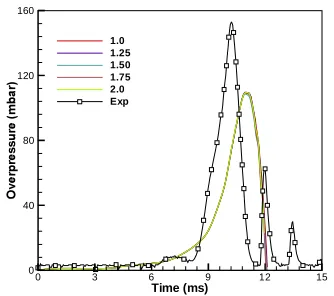
[image:7.595.85.248.80.531.2]Four additional LES simulations were carried out to verify the influence of filter width coefficient on numerical accuracy by varying the value of from 1.0 to 2.0 with an interval of 0.25. Fig. 10 shows the overpressure time histories from LES simulations using various filter coefficient values. It is interesting to note that LES predictions from all simulations are falling on same line and shows no sensitivity to the chosen Fig. 9 Sequence of images to show flame structure at
different times after ignition (a) Case G,(b) Case H, (c) Case I and (d) Experimental images from high speed video recordings. (a), (b) and (d) present at 6, 9.5, 10,
10.5 and 11ms and (c) at 6, 7, 7.6, 7.8 and 8ms (b)
(c) (a)
value. Fig.10 clearly indicates that, there is no significant improvement in the pressure-time history, by changing the value of the filter width coefficient. It can be seen that, the pressure time histories from the simulations using from 1.0 to 1.75 are overlapping when is equal to 2.0. As explained earlier, this phenomenon is due to the implicit filtering approach used in the present simulations.
It is also identified that, in governing the numerical accuracy, filter width has a restricted role due to the type of filtering approach employed, which is directly linked to the grid resolution. However, filter width determines the portion of turbulence kinetic energy resolved, irrespective of the type of filtering approach, which is another key ingredient for good LES. In the present investigation, calculations have been made to estimate the resolved turbulence kinetic energy (not shown here) which is adequate for a good LES simulation [3].
5. CONCLUSIONS
A number of LES simulations of propagating turbulent premixed flames, of propane/air mixture of equivalence ratio 1.0, past repeated obstacles have been carried out. The grid chosen for the present simulations has 2.7 million cells in computational domain and found to be adequate in resolving about 70% of the turbulent kinetic energy [3] for this configuration. The mean chemical reaction rate is modelled using a simple FSD model based on the flamelet approach.
Controlling parameters such as ignition radius, Bogers
constant, test filter to grid filter ratio ( ) and the filter width coefficient ( ) are systematically varied to understand their influence upon LES predictions. Results from LES simulations are compared against available experimental measurements and analysed. The following conclusions can be made from the above study.
The ignition radius was varied from 3 to 6 mm with initial reaction progress variable of 0.5 and 0.7. LES predictions were found to be very sensitive to the ignition radius and found to burn faster with higher ignition radius. Initial reaction progress variable within the ignition radius was found to be less sensitive compared to the ignition radius. A 4mm ignition radius with 0.5 reaction progress variable was found to mimic the initial quasi-laminar phase of the turbulent flame ignited from rest.
The test filter to grid filter ratio ( ) is found to have significant influence on LES predictions. Two values i.e. 1.362 and 2.0 were used here and LES predictions using = 2.0 were found to be in closest agreement with experimental measurement. Higher test filter to grid filter ratio can be attributed in resolving the more accurate momentum and scalar fluxes at test filter level, which were used to calculate sub-grid scale fluxes at grid filter level.
The value of Bogers constant ( ) was found to be very significant in altering the LES predictions. Three values i.e. 1.2, 1.4 and 1.8 were used here and LES predictions were found to be very sensitive. It was noticed that high sensitivity of LES predictions is directly related to higher
flame surface area due to high flame wrinkling. Bogers
constant above 1.4 seems to be predicting unrealistic results. Hence, it is advisable to use a value between 1.2 and 1.4.
Influence of the filter width coefficient ( ) has been studied by choosing 5 values between 1.0 and 2.0 with an increment of 0.25. It has been noticed that the LES predictions were insensitive to the value of . This is attributed to the type of grid filtering (box/top-hat) process considered in this study.
It can be concluded that the LES predictions in Case G having an ignition radius of 4.0mm, initial reaction progress variable of 0.5, test filter to grid filter ratio of 2.0 and filter width coefficient of 2.0 are in good agreement with experimental measurements. Predicted overpressure trend, flame position, flame speed and flame structure were found to be in good agreement with measurements. However, the difference in the overpressure trend between LES and measurements can be attributed to the simple FSD model used in this study.
[image:8.595.79.246.83.231.2]Finally, the key findings from this investigation are found to be in line with the values found in literature and give good confidence for further use.
Fig. 10 Pressure time histories from LES simulations with various filter coefficient values as shown in legend.
Time (ms)
0 3 6 9 12 15
0 40 80 120 160
ACKNOWLEDGMENTS
We wish to thank Prof. Assad Masri, The University of Sydney, Australia for helpful discussions and providing the experimental data.
REFERENCES
[1] A. R. Masri, S. S. Ibrahim and B. J. Cadwallader,
"Measurements and large eddy simulation of propagating premixed flames", Experimental Thermal and Fluid Science, vol. 30 (7), pp. 687-702, 2006.
[2] V. Di Sarli, A. Di Benedettoa, G. Russo, Using large
eddy simulations for understanding vented gas explosions
in the presence of obstacles, J. Hazard. Mater., vol. 169, pp. 435442, 2009.
[3] S. R. Gubba, S. S. Ibrahim, W. Malalasekera and A. R.
Masri, An assessment of large eddy simulations of
premixed ßames propagating past repeated obstacles,
Combust. Theory and Modelling, vol. 13 pp. 513-540, 2009.
[4] S. R. Gubba, S. S. Ibrahim, W. Malalasekera and A. R. Masri, LES modelling of premixed deflagrating flames
in vented explosion chamber with a series of solid
obstructions, Combust. Sci. Technol., vol. 180 (10) pp.
1936-1955, 2008.
[5] H. Pitsch, A consistent level set formulation for large-eddy simulation of premixed turbulent combustion,
Combust. Flame, vol. 143, pp. 587-598, 2005.
[6] S. B. Pope, Ten questions concerning the large-eddy
simulation of turbulentßows, New J. Phys., vol. 6(35), pp. 124, 2004.
[7] J. E. Kent, A. R. Masri, S. H. Starner and S. S. Ibrahim, A new chamber to study premixed flame propagation past repeated obstacles, in 5th Asia-Pacific Conference
on Combustion, The University of Adelaide, Australia, pp. 17-20, 2005.
[8] R. Hall, A. R. Masri, P. Yaroshchyk and S. S. Ibrahim, Effects of position and frequency of obstacles on
turbulent premixed propagatingßames, Combust. Flame,
vol. 156, pp. 439-446, 2009.
[9] J. Smagorinsky, General circulation experiments with the primitive equations, Monthly Whether Review, vol.
91, pp. 99-164, 1963.
[10] M. Germano, U. Piomeli, P. Moin and W. H. Cabot, A dynamic subgrid-scale eddy viscosity model, Phys,
Fluids, vol. A3 (7), pp. 1760-1765, 1991.
[11] P. Moin, K. Squires, W. H. Cabot and S. Lee, A dynamic
subgrid-scale model for compressible turbulence and
scalar transport, Phys. Fluids, vol. A3, pp. 27462757,
1991.
[12] K. N. C. Bray, Studies of turbulent burning velocity,
Proc. R. Soc. London, Ser. A, 431, p. 315, 1990.
[13] R. O. S. Prasad and J. P. Gore, An evaluation of flame surface density models for turbulent premixed jet flames,
Combust. Flame, vol. 116 (1-2), pp.1-14, 1991.
[14] M. Boger, D. Veynante, H. Boughanem and A. Trouve,
Direct numerical simulation analysis of flame surface
density concept for large eddy simulation of turbulent
premixed combustion, Proc. Combustion Institute, vol.
27 (1), pp. 917-925, 1998.
[15] K. N. C. Bray, M. Champion and P. A. Libby, Flames in stagnating turbulence, in Turbulent Reacting Flows. eds. Borghi R and Murphy S N (Springer Publications:
New York) pp 541- 563, 1989.
[16] M. P. Kirkpatrick, S. W. Armfield, A. R. Masri, and S. S.
Ibrahim, Large eddy simulation of a propagating
turbulent premixed flame, Flow turbulence and
combustion, vol. 70, pp. 1-19, 2003.
[17] S. R. Gubba, Development of a dynamic LES model for premixed turbulent flames PhD thesis, Loughborough
University, UK (2009).
[18] H. Werner, and H. Wengle, Large-eddy simulation of turbulent flow over and around a cube in a plate channel,
8th Symposium on Turbulent Shear Flows Munich, Germany, 1991.
[19] R. Hall, Influence of obstacle location and frequency on the propagation of premixed, M.E. thesis, The University of Sydney, Sydney (2008).
[20] D. Bradley and F. K. K. Lung, Spark ignition and the early stages of turbulent flame propagation, Combust.
Flame, vol. 69, pp. 71-93, 1987.
[21] U. Schumann, "Large-eddy simulation of turbulent diffusion with chemical reactions in the convective boundary layer", Atmospheric Environment, vol. 23 (8), pp. 1713-1727, 1967.
[22] F. K. Chow, and P. Moin, "A further study of numerical
errors in large-eddy simulations", Journal of
Large Eddy Simulation of Premixed Turbulent
V-Flame Using a V-Flamelet Generated Manifold (FGM)
based Combustion Model
P. Pantangi
1, F. Dinkelacker
2, M. Chrigui
1, A. Sadiki
11Darmstadt University of Technology, Department. of Mechanical Engineering, Energy and powerplant technology, Petersenstr.
30, 64287 Darmstat, Germany.
2Leibniz University of Hannover, Institute of Technical Combustion,
Welfengarten 1a, 30167 Hannover, Germany
Abstract: The present paper aims at an evaluation of the
ability of combustion-LES to correctly describe turbulent premixed combustion, especially a rod stabilized unconfined flame. For this purpose the flamelet generated manifold (FGM)-tabulated chemistry approach, in which a variable local equivalence ratio due to a possible entrainment of the environment air is included through a mixture fraction variable, is integrated into an appropriate complete model. To measure the accuracy of the numerical method, LES results of the rod stabilized flame are compared with experimental data. A satisfactory agreement for the flow field quantities and species concentrations is achieved along with an assessment of the SGS scalar flux model used.
Keywords:Premixed combustion; FGM; SGS fluxes
1. INTRODUCTION
Turbulent premixed combustion plays an important role in many technical applications, e.g., in spark ignition engines and in gas turbines. While RANS computations of premixed flames are well reported in the literature, LES of premixed combustion remains difficult due to the thickness of the premixed flame
about 0.11 mm and generally smaller than the LES mesh size.
Physical and chemical features of combustion LES have been discussed by Janicka and Sadik [1], and Pitsch [2] with emphasis focused on important aspects of an overall model. Several approaches have been reviewed for modeling of premixed turbulent combustion; this comprehends turbulence controlled models (eddy break up, eddy dissipation models), statistical approach based models (PDF Transport equations, CMC, etc.), flamelet based models (surface Density models, G-equations, BML based models) or artificially thickened flame (ATF) approach. With regard to chemistry, the detail of chemistry is unavoidable if one has to address auto-ignition, flame stabilization, recirculating products which may include
intermediate species, and the prediction of some pollutants [3,4,5]. The reduction and tabulation of chemical species behavior prior to LES remains one of the available options that is being investigated to downsize combustion chemistry in order to make it compatible with flow solvers.
Efforts to extend the applicability of LES technique to premixed turbulent flame description are pursued here. To account for kinetic effects and flame stabilization in this work, the flamelet generated manifolds (FGM) method is introduced [5,6] and coupled to LES. This is achieved by incorporating into the CFD an additional transport equation for the progress variable besides the mixture fraction equation and the classical flow governing equations. The resulting complete model is applied to simulate a laboratory-scale turbulent V-flame for which comprehensive experimental data are available.
A V-shape flame is generated when a premixed flame is stabilized on a hot wire or a rod [7] . In a laminar flow environment, the reaction layer propagates against the incoming fluid and a premixed V-shape flame is built. In the case of a turbulent flow, the two wings of the flame are wrinkled by velocity fluctuations and the V-flame is obtained in mean (see Fig.1). As pointed out by Domingo et al. [8] the flame stabilized by the rod takes benefit from the recirculation of hot products behind the obstacle, while the flame stabilized on a hot wire is initiated by the energy released by the wire. Thereby the very localized burning kernel serves to stabilize a premixed flame that develops downstream. Besides 2D DNS [8] and 3D DNS [9] calculations for low Reynolds number configurations, LES of V-flame are very rare. Manickam et al. [10] applied an algebraic flame surface wrinkling model to study rod stabilized flames. They compared the performance of a RNG k-Epsilon RANS model and a standard Smagorinsky LES using the commercial code Fluent to address the flow past