promoting access to White Rose research papers
White Rose Research Online
Universities of Leeds, Sheffield and York
http://eprints.whiterose.ac.uk/
This is an author produced version of a paper published in Communications in Computational Physics.
White Rose Research Online URL for this paper: http://eprints.whiterose.ac.uk/7947/
Published paper
Baines, M.J., Hubbard, M.E., Jimack, P.K. and Mahmood, R. (2009) A moving-mesh finite element method and its application to the numerical solution of phase-change problems. Communications in Computational Physics, 6 (3). pp. 595-624.
A Moving-Mesh Finite Element Method and its
Application to the Numerical Solution of Phase-Change
Problems
M.J. Baines
Department of Mathematics, The University of Reading, UK
M.E. Hubbard
P.K. Jimack
School of Computing, University of Leeds, UK
R. Mahmood
Computer Division, Pakistan Institute of Nuclear Science
and Technology (PINSTECH), Islamabad, Pakistan
A distributed Lagrangian moving-mesh finite element method is applied to problems involving changes of phase. The algorithm uses a distributed conservation principle to de-termine nodal mesh velocities, which are then used to move the nodes. The nodal values are obtained from an ALE (Arbitrary Lagrangian-Eulerian) equation, which represents a
gener-alisation of the original algorithm presented in Applied Numerical Mathematics, 54:450–469
(2005). Having described the details of the generalised algorithm it is validated on two test cases from the original paper and is then applied to one-phase and, for the first time, two-phase Stefan problems in one and two space dimensions, paying particular attention to the implementation of the interface boundary conditions. Results are presented to demonstrate the accuracy and the effectiveness of the method, including comparisons against analytical solutions where available.
1
Introduction
singularities and moving boundaries) [2, 5, 6, 7, 10, 18, 30, 31, 32, 33, 42, 43, 44], and/or to exploit geometric properties such as scale-invariance, orderings or asymptotics [8, 12, 15]. The moving-mesh methods can be divided into two broad categories: those based on mappings between a fixed computational mesh and physical space [10, 16, 17, 38] and those based on velocities expressed in terms of the mesh coordinates in physical space [6, 12, 18, 19, 20, 34]. In this paper we focus on one particular velocity-based moving-mesh finite element method [6, 7, 8], which is related to the Geometric Conservation Law [18, 40]. This method has been successfully applied to a range of time-dependent nonlinear PDE problems involving singularities and implicit moving boundaries: however, since its original introduction in [6], a number of improvements have been made which are incorporated into the description below. The algorithm has been designed to be very general in nature and applicable to a large family of problems. Having validated the proposed method for a range of situations, the main thrust of this paper is its application, for the first time, to phase-change problems involving an internal moving boundary. Many numerical schemes have been applied to such problems, including those involving moving-mesh techniques [10, 25, 26, 33, 39]. The application of the moving-mesh finite element method described in this paper to this problem is however new, and is shown to be both accurate and robust.
The layout of the paper is as follows. Section 2 gives a description of the moving-mesh finite element method of [6] incorporating a number of recent developments. Section 3.1 presents validating results from a mass-conserving problem using the porous medium equa-tion [41], which is a second order nonlinear diffusion equaequa-tion for which simple self-similar solutions exist with finite support that grows with time. Section 3.2 then describes validating results from a non-mass-conserving implicit moving boundary problem, a simple model of absorption and diffusion, referred to here as the Crank-Gupta problem [24], which contains a sink term which causes the finite support to shrink with time. Section 4 contains the main application of the moving-mesh finite element method to one-phase and two-phase Stefan problems and section 5 contains details of the results of numerical experiments, validated against analytic solutions whenever possible. Finally, section 6 includes a discussion of points raised in the paper.
2
A Moving-Mesh Finite Element Method
2.1
A Mesh Movement Velocity Potential
Letu(x, t) be the solution of a well-posed time-dependent nonlinear PDE problem of general
form
∂u
∂t = Lu (1)
on a finite time-dependent domain R(t), where L is a differential operator involving space
derivatives only, with consistent boundary conditions on the (in general moving) boundary
∂R(t).
An important quantity in our approach is the total integral of the dependent variable
θ(t) = Z
R(t)
u dx. (2)
For brevity and convenience we will refer to θ(t) as the “mass” in the domain at time t.
Note however that, as in section 4 for example, the dependent variable may be related to a quantity other than density.
A moving polygonal or polyhedral approximation R(t) to R(t), with boundary ∂R(t)
approximating ∂R(t), is assumed, together with a moving tessellation of simplices of R(t).
A piecewise linear approximation U is also assumed, which can be expanded in terms of
piecewise linear basis functions Wi(t,x) forming a partition of unity and moving with the
domain. The total discrete mass Θ(t)≈θ(t) is defined by (cf.(2))
Θ(t) =
Z
R(t)
U dx. (3)
Now consider the distribution of the mass (3) across the domain R(t). Each basis function
Wi(t,x) is associated with a partial mass and a proportion Ci, defined by
Z
R(t)
WiU dx = CiΘ(t) = Ci
Z
R(t)
U dx. (4)
A moving-mesh numerical method can be created by keeping the proportionsCi ∈[0,1]
constant as time progresses. The fact that the weight functions Wi(t,x) are non-negative
and form a partition of unity means that conservation of the partial masses (4) is consistent
with total mass conservation. (Clearly PCi = 1 is required to maintain the correct total
mass and this also follows from PWi ≡1.)
The velocityV(t,x) of the moving frame can be derived from a weak form of the Reynolds
Transport Theorem [6],
d dt
Z
R(t)
WiU dx
=
Z
R(t)
∂(WiU)
∂t +∇ ·(WiUV)
dx
= Z
R(t)
Wi
∂U
∂t +∇ ·(UV)
dx, (5)
since we have assumed that the basis functions Wi(t,x) move with the domainR(t) and are
therefore advected with velocity V,i.e.
∂Wi
From (5) and a weak form of (1) a moving weak form of the PDE can be written as
d dt
Z
R(t)
WiU dx
−
Z
R(t)
Wi∇ ·(UV)dx =
Z
R(t)
WiLU dx, (7)
where the U on the right hand side may need to be regularised to lie in the domain ofL.
Hence, applying (4) with constant Ci, equation (7) gives
CiΘ˙ −
Z
R(t)
Wi∇ ·(UV)dx =
Z
R(t)
WiLU dx. (8)
A unique solution of equation (8) for V in multiple space dimensions is obtained if the
curl of V is prescribed in R(t) and the normal component of V is prescribed on ∂R(t),
by Helmholtz’ Theorem. For ease of exposition we shall assume that curl V = 0, so that
V =∇Φ, where Φ is a scalar velocity potential.
Instead of (8), Φ and ˙Θ now satisfy the equation
CiΘ˙ −
Z
R(t)
Wi∇ ·(U∇Φ) dx =
Z
R(t)
WiLU dx (9)
or, after integration by parts,
CiΘ˙ −
I
∂R(t)
WiU∇Φ·nds +
Z
R(t)
U∇Φ· ∇Wi dx =
Z
R(t)
WiLU dx, (10)
where n is the unit outward normal to ∂R(t), the boundary of the domain.
Summing equations (10) over all of the mesh nodes gives
˙
Θ −
I
∂R(t)
U∇Φ·n ds = Z
R(t)
LU dx, (11)
which, in situations where UV·n is known on the entire boundary, can be used to give an
explicit expression for ˙Θ. However, for greater generality, the rate of change of mass ˙Θ is
treated here as an unknown.
Combining (10) with (11) yields a square system of equations of reduced rank, since equation (11) is the sum of equations (10). Although the combined system has a single
infinity of solutions, a unique solution for Φ and ˙Θ may be obtained by specifying the value
of Φ at one of the nodes and ignoring the corresponding equation. Since Φ is a velocity potential there is no resulting loss of generality. Although we do not do so in this paper, a
further option is to impose a constant value of Φ on the whole of∂R(t), which has the effect
of weakly specifying zero tangential velocity of the boundary nodes.
The nodal velocities V may be recovered from Φ by minimising the L2 norm of each
component of V− ∇Φ, leading to the vector equation
Z
R(t)
WiV dx =
Z
R(t)
Wi∇Φdx, (12)
for all nodes i. Having foundV and ˙Θ, the nodal positions X as well as Θ can be advanced
The values of the solution U can then be recovered either by direct inversion of equation (4) or, more generally, by the use of a conservative Arbitrary Lagrangian-Eulerian (ALE) equation of the form
d dt
Z
R(t)
WiU dx
=
Z
R(t)
Wi (LU+∇ ·(UV)) dx (13)
(cf. equation (7)), which gives the consistent form of the integral
Z
R(t)
WiU dx (14)
prior to its inversion for U (but see equations (15) and (16) below).
So far, boundary conditions for the dependent variableU have not been discussed. In
cir-cumstances where the methodology is designed to conserve mass (with appropriate boundary
conditions on V), the numerical method should do the same with the discrete form of the
mass. However, the standard way of imposing Dirichlet boundary conditions in the finite
element inversion of (14) for U destroys mass conservation in general (since the test
func-tions corresponding to nodes on the Dirichlet boundary are not used and so the remaining test functions no longer form a partition of unity). In [29] a modification is proposed which retains mass conservation in the presence of strongly imposed Dirichlet boundary conditions, and moreover is shown to improve the accuracy of the method. This is achieved by defining
a set of modified test functions fWi used in the recovery of the nodal values of the dependent
variable U.
We shall therefore recover U values from modified partial masses Ψi(t), defined by (cf.
equation (4))
Ψi(t) =
Z
R(t)
f
WiU dx, (15)
using the discrete form of the ALE equation (cf. equation (13))
˙
Ψi =
Z
R(t)
f
Wi (LU +∇ ·(UV)) dx (16)
(for those mesh nodes at which Dirichlet boundary conditions are not applied). Although
they both represent rates of change of partial masses associated with mesh nodes,CiΘ and ˙˙ Ψi
are different quantities in the discrete algorithm. The former are calculated to be consistent
with the velocity field represented by ∇Φ while the latter are consistent with the actual
nodal velocities V, as derived using (12). The rate of change of total mass of the system is
governed by the ALE equation (16) used to update the dependent variable so, from now on,
Ψ(t) =
Z
R(t)
U dx (17)
2.2
Algorithm
The algorithm used in this paper for a single time-step can now be summarised as follows:
1. Given a set of mesh nodes with positions Xi and a distribution of the total mass Ψ,
defined by the masses Ψi of (15), to all those mesh nodes where Dirichlet boundary
conditions are notapplied, invert (15) to recover the solution values U at these nodes.
(The Dirichlet conditions on U are imposed at the remaining nodes.)
2. Having found the nodal values Ui, solve the set of equations (10) and (11) for the
velocity potentials Φiand for ˙Θ, imposing Φ at one mesh node. Note that the constants
Ci must be recalculated from (4) before this step can be carried out.
3. Use the resulting values of Φi to obtain the mesh node velocities Vi from (12) for all
mesh nodes, either with or without imposing boundary conditions on V.
4. Knowing V (= ˙X), obtain the corresponding adjustments to the local masses (15)
using the ALE equation (16), thus computing the ˙Ψi values.
These four steps can be thought of as evaluating a vector function of the formF~(X~, ~Ψ) (the
arrows indicating a vector which contains the values stored at all the nodes of the mesh) which satisfies
d(X~, ~Ψ)
dt = F~(X~, ~Ψ). (18)
This system of ordinary differential equations in time can then be integrated using any convenient time-stepping scheme. Here, following the investigation presented in [29], Heun’s scheme is used. Experiments recorded there demonstrated that Heun’s scheme ensures that the error in the temporal discretisation is negligible compared to the error in the spatial discretisation for almost any (stable) time-step which avoids mesh tangling.
2.3
Comparison
The moving-mesh finite element method presented above is essentially that presented in [6] but with the following modifications:
• Instead of recovering the values of U on the new mesh directly from the conservation
principle (4), an ALE equation (16) is used prior to using (15) to update U. This
allows the extension of the method to more general monitor functions.
• The partial masses Ψi used to drive the mesh movement are updated using the ALE
equation (16), so the distribution of the mass defined by the coefficients Ci in (4) is
• The rate of change of the conserved quantity ˙Θ is treated in equations (10) and (11) as an unknown and calculated at each time-step (although now it is only ever used as
a means to find Φ). This provides additional generality since ˙Θ may not always be
available explicitly.
• Dirichlet boundary conditions are imposed strongly in a way which conserves mass
when the underlying system does, using the modified test functions Wfi of [29].
• To ensure that the system has a unique solution when solving for the mesh velocity
potentials, Φ is imposed at just one mesh node, whereas in the previous work Φ was always specified over the whole boundary. This removes a potentially unnecessary constraint on Φ.
• Heun’s scheme, an explicit, two-stage, second order, TVD Runge-Kutta method is used
to discretise the time derivative instead of the forward Euler scheme used in [6]. This offers improved temporal accuracy [29].
3
Method Validation
Two sets of numerical tests have been carried out to validate the method, in one and two space dimensions. The first set of tests is carried out on the porous medium equation, a second order nonlinear diffusion problem for which mass is conserved globally. The second set is on a linear diffusion equation with a source/sink term representing absorption, for which mass is not conserved. The results are validated against exact solutions and can be compared with those presented in [6].
Both sets of calculations have been carried out on meshes which are initially uniform, and for which the representative initial mesh size is repeatedly halved to estimate orders of accuracy. Mesh tangling is avoided by dividing the time-step by four with each refinement. The initial conditions sample the exact nodal values of the dependent variable at the nodes. In sections 3 and 4 it will be necessary to distinguish between different types of boundary.
Fixed parts of the boundary will be denoted by ΓF, at which the condition V·n = 0 is
imposed, where n is a normal to the boundary. Implicit moving parts of the boundary,
where no such condition is imposed, will be denoted by ΓM(t). In both cases the boundary
conditions imposed on U will depend on the problem being solved.
Furthermore, in all of the test cases presented, a condition forU∇Φ·n is given on every
boundary. Hence, ˙Θ is actually known explicitly, and it is only necessary to specify Φ at
one point. Nevertheless, for the sake of generality, we choose to treat ˙Θ as an unknown
when calculating the Φi and we thus specify Φ = 0 at one point. This point can be chosen
3.1
A Mass-Conserving Nonlinear Diffusion Problem
The porous medium equation, details of which can be found in [3, 41], is given by
∂u
∂t = ∇ ·(u
n
∇u) in R(t), (19)
where n > 0 is an integer exponent. A Dirichlet boundary condition u = 0 is imposed on
the moving boundary ΓM(t). For this problem it can be shown that mass, as defined by (2),
is conserved.
For this problem the operator Lu≡ ∇ ·(un∇u) and equation (10) gives
CiΘ +˙
Z
R(t)
U∇Φ· ∇Wi dx =
I
ΓF
WiUn∇U ·n ds −
Z
R(t)
Un∇Wi· ∇U dx (20)
since U = 0 on the moving boundary ΓM(t) and V·n = 0 on ΓF. Similarly, equation (11)
becomes
˙ Θ =
I
ΓF
Un∇U·n ds . (21)
Equations (20) and (21) give ˙Θ and the velocity potential Φ, which is used in (12) to find
the mesh velocity V = ˙X. The discrete ALE equation (16) becomes
dΨi
dt =
Z
R(t)
f
Wi {∇ ·(Un∇U) +∇ ·(UV)} dx (22)
which, after integration by parts and imposition of the boundary conditions, gives
dΨi
dt =
I
ΓF
f
WiUn∇U ·nds −
Z
R(t)
∇Wfi·(Un∇U +UV)dx. (23)
Heun’s method is used to update X~ and Ψ, and inversion of equation (15) to recover the~
dependent variable U. In all of the following cases ΓF = ∅, so the boundary integrals in
equations (20)–(23) disappear and ˙Θ = 0 is known explicitly.
Equation (19) admits a family of exact compactly supported similarity solutions with
moving boundaries on which u = 0 [9, 35]. In d space dimensions a radially-symmetric
self-similar solution exists of the form
u(r, t) =
1 λd(t)
1−r r
0λ(t)
2n1
r ≤r0λ(t)
0 r > r0λ(t)
(24)
in which r≥0 is the usual radial coordinate, and where
λ(t) =
t t0
1
2+dn
and t0 =
r02n
2(2 +dn). (25)
The problem is parameterised by the initial front position r0 (at time t0) and the position
−2.5 −2 −1.5 −1 −6
−5 −4 −3 −2
LOG(dx)
LOG(error)
Porous Medium Equation: n = 1
ALE solution
ALE mesh slope = 2
−2.5 −2 −1.5 −1
−4 −3 −2 −1
LOG(dx)
LOG(error)
Porous Medium Equation: n = 3
ALE solution
[image:10.612.77.518.11.229.2]ALE mesh slope = 1
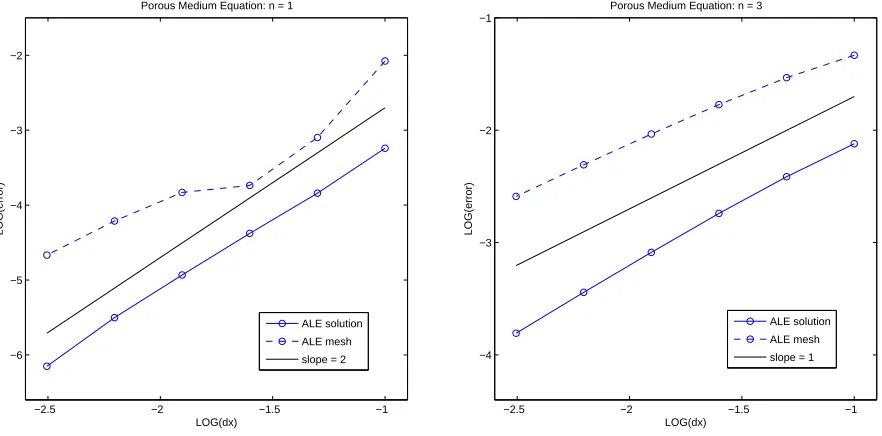
Figure 1: Comparison of L2 errors in the solution and the magnitudes of the errors in the
boundary node positions for the porous medium equation in one space dimension withn = 1
(left) and n= 3 (right).
Two instances of (19) are considered here, one with exponent n= 1 (for which the slope
of the self-similar solution normal to the moving boundary is finite) and another with n = 3
(for which the slope normal to the boundary is infinite). The test cases are run until time
T = t− t0, as detailed below. Results have been computed in both one and two space
dimensions for each test case as follows.
• One dimension, n = 1, r0 = 0.5, t0 = 0.04167, run until T = 10 (when r≈3.11154).
• One dimension, n = 3, r0 = 0.5, t0 = 0.075, run until T = 10 (whenr ≈1.33231).
• Two dimensions, n = 1, r0 = 0.5, t0 = 0.03125, run until T = 0.1 (when r≈ 0.71578).
• Two dimensions, n= 3,r0 = 0.5,t0 = 0.046875, run untilT = 0.1 (when r≈0.57673).
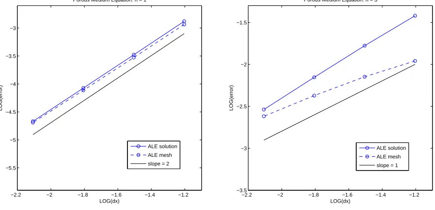
The values of various discrete error measures are shown in Figures 1 and 2. The results
exhibit approximately second order accuracy when n = 1, which reduces to first order when
n = 3, as in [6].
3.2
A Non-Mass-Conserving Diffusion Problem with a Source
The Crank-Gupta problem [11, 24, 36] provides an example of a problem where the total mass of the system changes due to the presence of a source/sink term. The problem is defined by the differential equation
∂u
∂t = ∇
2u
−2.2 −2 −1.8 −1.6 −1.4 −1.2 −5.5
−5 −4.5 −4 −3.5 −3
LOG(dx)
LOG(error)
Porous Medium Equation: n = 1
ALE solution
ALE mesh
slope = 2
−2.2 −2 −1.8 −1.6 −1.4 −1.2
−3.5 −3 −2.5 −2 −1.5
LOG(dx)
LOG(error)
Porous Medium Equation: n = 3
ALE solution
ALE mesh
[image:11.612.76.518.14.227.2]slope = 1
Figure 2: Comparison ofL2 errors in the solution and boundary node positions for the porous
medium equation in two space dimensions with n= 1 (left) and n= 3 (right).
with boundary conditions u= 0 and ∂u/∂n= 0 on the moving boundary ΓM(t).
For this problem Lu≡ ∇2u−1 and, after integration by parts, equation (10) becomes
CiΘ +˙
Z
R(t)
U∇Φ· ∇Wi dx
= I
ΓF
Wi∇U ·nds −
Z
R(t)
∇Wi· ∇U dx −
Z
R(t)
Wi dx, (27)
since V · n = 0 on the fixed boundary and U = ∇U · n = 0 at the moving boundary.
Furthermore, summing (27) over the whole domain gives
˙ Θ =
I
ΓF
Wi∇U ·nds −
Z
R(t)
dx. (28)
The discrete ALE equation (16), after integration by parts and imposition of the boundary conditions, gives
dΨi
dt =
I
ΓF
f
Wi∇U ·nds −
Z
R(t)
∇fWi·(∇U +UV)dx −
Z
R(t)
f
Wi dx. (29)
Heun’s method is again used to updateXand Ψi, after which equation (15) is used to recover
U. The results summarised below are obtained with Ux specified at x= 0.
In [11] an exact solution to the one-dimensional equation on the interval [0, x(t)] with the
same boundary conditions at the moving boundary, but with ux(0, t) =−1 +et
−1
at x= 0,
is given as
u(x, t) = (
−x−t+ex+t−1
x≤1−t
−2.5 −2 −1.5 −1 −8
−7 −6 −5 −4 −3
LOG(dx)
LOG(error)
Absorption−Diffusion Problem
ALE solution
[image:12.612.190.401.12.227.2]ALE mesh slope = 2
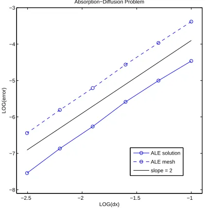
Figure 3: Comparison of L2 errors in the solution and the magnitudes of the errors in the
boundary node positions for the absorption-diffusion problem in one space dimension.
with initial condition u(x,0) = −x +ex−1
for x ∈ [0,1] at t = 0. Results for this test
case have been compared with the exact solutions at t = 0.6. The values of various error
measures are shown in Figure 3. The results match those of [6], giving second order accurate approximations to both solution and boundary position.
Two-dimensional calculations are not presented here due to the lack of an analytical solution to compare with. It is simply noted that the new scheme appears to be more robust than the original one proposed in [6], since it is possible to run the numerical experiment described there for a significantly longer time with the improved method, taking the solution far closer to the point where the mass vanishes before mesh tangling occurs.
We now turn attention to the main purpose of this paper, which is to demonstrate that the moving-mesh finite element method described here may be applied to problems with change of phase at internal boundaries, in addition to the problems with exterior moving boundaries already considered.
4
Stefan Problems and Changes of Phase
The two-phase problem will be presented first, for which the phase-change is modelled by
applying the Stefan condition at a moving internalboundary. The single-phase problem will
4.1
The Two-Phase Problem
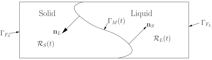
Consider a domain divided into regions of solid or liquid phase, denoted respectively byRS(t)
and RL(t). This is illustrated for a domain split into two regions in Figure 4. As indicated,
the boundary of the solid region is divided into two components, the moving interface with
the liquid phase ΓM(t) and a fixed part ΓFS, which in Figure 4 coincides with the external
boundary of the domain. The boundary of the liquid region is similarly divided between
ΓM(t) and ΓFL. For simplicity, only two regions will be considered: all of the test cases
investigated here (in two dimensions) have one region completely inside the other, although it should be noted that this is not a restriction of the method.
Solid
Liquid
Γ
FSR
S(
t
)
R
L
(
t
)
Γ
FLΓ
M(
t
)
n
S [image:13.612.92.525.191.314.2]n
LFigure 4: A representative domain, with our notation, for the two-phase Stefan problem.
The two-phase Stefan problem (described in detail in [23]) models the transition of some substance between liquid and solid phases. This process takes place across an interface in the interior of the problem domain which moves as time progresses. It is modelled by the equations [13]
KSut = ∇ ·(kS∇u) in RS(t)
KLut = ∇ ·(kL∇u) in RL(t), (31)
in which KS, KL represent the volumetric heat capacities, kS, kL the thermal conductivities
and u the temperature. The interface conditions are u = uM and, based upon an energy
balance across the phase-change boundary ΓM(t),
kS∇uS·n−kL∇uL·n = λv·n, (32)
where n =n(t) is a normal to the moving interface, λ is the heat of phase-change per unit
volume, and v·n is the normal velocity of the interface. All parameters are assumed here
to be constant within their respective phases. In the (Stefan) condition (32), the derivative
∇u·nis discontinuous across the moving interface (althoughuis continuous) and subscripts
Note that the entire problem (including the evolution of the interface) is unchanged by
the addition of a constant value to u throughout the domain (as well as to uM and the
Dirichlet boundary conditions on ΓFS and ΓFL).
4.2
The Numerical Method
A moving polygonal approximation R(t) to R(t) = RS(t) ∪ RL(t) is set up, consisting
of a moving tessellation of simplices with piecewise linear fixed and moving boundaries
approximating ΓF = ΓFS∪ΓFL and ΓM(t), respectively. The individual stages of the method
can be described as follows.
4.2.1 Calculating the mesh velocity potential
Differentiating the weak form (4) with respect to time still results in (10), but substitution
for Lu from equation (31) leads to
CiΘ˙ −
I
ΓM(t)
WiU∇Φ·nds +
Z
R(t)
U∇Φ· ∇Wi dx
= κ
I
ΓF
Wi∇U ·nds − κ
Z
R(t)
∇Wi· ∇U dx (33)
after integration by parts, where κ=k/K takes a different value in each of the two phases.
We consider the solid and liquid phases separately. Dividing the domain between its
component phases leads to two discrete “masses” (cf. equation (3)),
ΘS(t) =
Z
RS(t)
U dx and ΘL(t) =
Z
RL(t)
U dx (34)
and, since V·n= 0 on ΓF and U =UM on ΓM(t), the two corresponding equations (33) for
the velocity potentials are, in the solid region,
CiSΘ˙S − UM
I
ΓM(t)
Wi∇Φ·nS ds +
Z
RS(t)
U∇Φ· ∇Wi dx (35)
= κS
I
ΓM(t)
Wi∇US·nS ds + κS
I
ΓFS
Wi∇U ·nds − κS
Z
RS(t)
∇Wi· ∇U dx
and in the liquid region,
CiLΘ˙L − UM
I
ΓM(t)
Wi∇Φ·nLds +
Z
RL(t)
U∇Φ· ∇Wi dx (36)
= κL
I
ΓM(t)
Wi∇UL·nLds + κL
I
ΓFL
Wi∇U ·nds − κL
Z
RL(t)
∇Wi · ∇U dx.
In these equations n always represents the outward pointing normal to the relevant domain
and, as illustrated in Figure 4,nL =−nS. This implies that Φ is dual-valued on the moving
interface ΓM(t), but this is not a problem because the recovery of ˙X from Φ in (12) in each
The Stefan condition (32) has not yet been used. We shall write it in a distributed form, consistent with the velocity potential equations (35) and (36), given by
kS
I
ΓM(t)
Wi∇US·nds − kL
I
ΓM(t)
Wi∇UL·nds = λ
I
ΓM(t)
Wi∇Φ·nds , (37)
for each node i on the interface ΓM. Recall that ∇U is discontinuous across the interface,
the subscripts S and L being used to denote the limiting values on either side in the solid
and liquid phases respectively.
Provided that UM 6= 0 and the dependent variable U does not change sign at any point
in the whole domain (which may always be achieved by the addition of a suitable constant to the whole system), it is possible to apply the boundary condition (37) by replacing the
terms involving ∇Φ·n in the integrals along the moving interface on the left-hand sides of
(35) and (36), giving
CiSΘ˙S +
Z
RS(t)
U∇Φ· ∇Wi dx
= κS
I
ΓM(t)
Wi∇US·nS ds + κS
I
ΓFS
Wi∇U ·nds − κS
Z
RS(t)
∇Wi· ∇U dx
+ UM
λ
I
ΓM(t)
Wi(kS∇US−kL∇UL)·nS ds (38)
for the solid region and
CiLΘ˙L +
Z
RL(t)
U∇Φ· ∇Wi dx
= κL
I
ΓM(t)
Wi∇UL·nLds + κL
I
ΓFL
Wi∇U ·nds − κL
Z
RL(t)
∇Wi · ∇U dx
+ UM
λ
I
ΓM(t)
Wi(kS∇US−kL∇UL)·nLds (39)
for the liquid region.
Equations (38) and (39) can each be summed to obtain two additional equations, giving the rate of change of the total mass in each phase:
˙
ΘS = κS
I
ΓM(t)∇
US·nS ds + κS
I
ΓFS ∇
U·n ds
+ UM
λ
I
ΓM(t)
(kS∇US −kL∇UL)·nS ds , (40)
˙
ΘL = κL
I
ΓM(t)∇
UL·nL ds + κL
I
ΓFL∇
U ·nds
+ UM
λ
I
ΓM(t)
(kS∇US −kL∇UL)·nL ds . (41)
Following the procedure used for a single domain, the values of Φi and ˙ΘS can be found by
solving (38) and (40) with the assumption that Φi = 0 at an arbitrary node i in the solid
region. Similarly, (39) and (41) can be solved for Φi and ˙ΘLwith the assumption that Φi = 0
4.2.2 Calculating the mesh velocity
The simplest way to recover the mesh velocities is to solve (12) forV, exactly as for a single
domain, except with V = 0 imposed on ΓF. While this procedure produces good
approx-imations, it is significantly more accurate to impose the Stefan condition (32) explicitly in
the recovery of V in (12). A single system is solved over the whole domain and, as before,
an equation of the form (12) is constructed for each interior node, and Vi = 0 imposed at
all nodes on the fixed boundary, but for those nodes on the moving interface the equations (12) are replaced using (37), which gives the normal components of the velocity directly. It
is assumed also that U = UM is constant along the moving interface, so ∇U is parallel to
n, and that the boundary nodes can only move in a direction perpendicular to the
bound-ary. Under these circumstances, the resulting equations solved at the nodes on the moving interface take the form
λ
I
ΓM(t)
WiVds = kS
I
ΓM(t)
Wi∇US ds − kL
I
ΓM(t)
Wi∇ULds . (42)
4.2.3 Recovering the dependent variable
The dependent variable U is recovered separately in each of the regions of the domain,
RS and RL, since they are decoupled by the Dirichlet boundary condition imposed on the
interface. A robust algorithm is obtained by using the ALE equation given by (16) to recover
the nodal values of the dependent variable. If ΨS
i and ΨLi are the local masses in the solid
and liquid phases (cf. equation (15)) we obtain
dΨS i
dt =
I
ΓM(t)
f
Wi(κS∇US+UMV)·nS ds + κS
I
ΓFS
f
Wi∇U ·n ds
−
Z
RS(t)
∇fWi·(κS∇U +UV)dx,
dΨL i
dt =
I
ΓM(t)
f
Wi(κL∇UL+UM V)·nLds + κL
I
ΓFL
f
Wi∇U ·nds
−
Z
RL(t)
∇Wfi·(κL∇U +UV)dx, (43)
where fWi are the modified test functions of section 2 which allowU to be specified strongly
on Dirichlet boundaries. The values of ΨS
i(t) and ΨLi (t) are then updated to the new time
level by the time-stepping scheme, after which they can be substituted into Z
RS(t)
f
WiU dx = ΨSi and
Z
RL(t)
f
WiU dx = ΨLi (44)
(cf. equation (15)) to find the new values for the dependent variable.
4.3
The One-Phase Problem
The single-phase Stefan problem is simply a special case of the two-phase problem described
region adjacent to the moving interface. This simplifies the equations considerably since only the liquid or the solid phase exists. For example, if the solid phase is being modelled then
the equations to be solved for the mesh velocity potentials are given by (38) with ∇UL = 0.
Regardless of whether a solid or a liquid phase is being modelled, in the single-phase case the interface condition (32) reduces to
k∇u·n = λv·n on ΓM(t). (45)
(Note however that the sign of k/λwill depend on the phase being modelled.) This leads to
the following equations:
k
I
ΓM(t)
Wi∇U ·nds = λ
I
ΓM(t)
Wi∇Φ·nds (46)
in place of (37),
CiΘ +˙
Z
R(t)
U∇Φ· ∇Wi dx (47)
= κ
I
∂R(t)
Wi∇U ·nds − κ
Z
R(t)∇
Wi· ∇U dx +
k UM
λ
I
ΓM(t)
Wi∇U ·nds
in place of (38)/(39),
˙
Θ = κ
I
∂R(t)
∇U·n ds + k UM
λ
I
ΓM(t)∇
U ·nds (48)
in place of (40)/(41), and
dΨi
dt =
I
ΓM(t)
f
Wi(κ∇U +UM V)·nds + κ
I
ΓF
f
Wi∇U·n ds
−
Z
R(t)
∇fWi·(κ∇U +UV)dx (49)
in place of (43).
5
Numerical Experiments
Throughout this section, unless stated otherwise, a constant value of δ = 2 is added to
the initial and boundary conditions to allow the Stefan boundary condition to influence the evolution and ensure that the solution is positive throughout the whole domain.
5.1
Single-Phase Results
5.1.1 One dimension
The first case considered is the one-dimensional single-phase example discussed in detail in
The single-phase problem permits each of the following analytic solutions on the domain
indicated which satisfy the Stefan condition at x =V t (the point at which ui =uM) when
λ =−1:
u(1)(x, t) = −1 +e−V(x−V t)
for x≤V t
and u(2)(x, t) = −1 +e−V(x−V t)
for x≥V t . (50)
Clearly V is the (constant) interface velocity and, in this case, UM = 0. Two situations are
examined here, both of which use a value of V =−1.
• Given the initial domain of [−1,0] and initial conditions given by u(1) at t
0 = 0, a
contracting domain is modelled with u ≤ 0 in the whole region. The choice k/λ < 0
implies that this is modelling the liquid phase, so it actually represents a supercooled
liquid, which is freezing at the moving interface, since V <0.
• Given the initial domain of [0,1] and initial conditions given by u(2) at t
0 = 0, an
expanding domain is modelled with u≥0 in the whole region. Again k/λ <0 implies
that this is modelling the liquid phase, which is melting the adjacent solid at the
moving interface, since V <0.
In each caseux =−V e
−V(x−V t)
is imposed as a Neumann condition on the fixed boundary in the calculation of the mesh velocity potentials. Note that there are analogous exact solutions
for the case where k/λ >0.
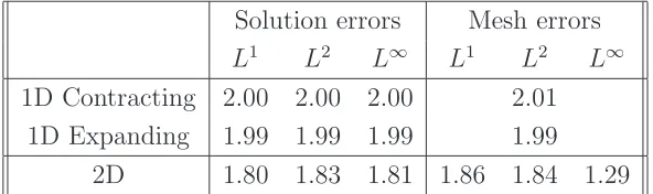
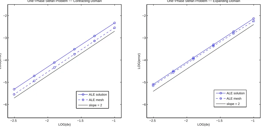
The results shown in Figure 5 and Table 1 clearly show that the overall method is second order accurate for the one-dimensional problem. Note that, for this one-dimensional problem,
the “mesh error” (i.e. the error in the position of the moving interface at the final time) is
[image:18.612.150.446.514.602.2]the same in each of the norms considered since the interface is just a single point.
Table 1: Numerical estimates of the orders of accuracy of the scheme applied to the single-phase Stefan problem.
Solution errors Mesh errors
L1 L2 L∞
L1 L2 L∞
1D Contracting 2.00 2.00 2.00 2.01
1D Expanding 1.99 1.99 1.99 1.99
−2.5 −2 −1.5 −1 −6
−5 −4 −3 −2
LOG(dx)
LOG(error)
One−Phase Stefan Problem −− Contracting Domain
ALE solution
ALE mesh
slope = 2
−2.5 −2 −1.5 −1
−6 −5 −4 −3 −2
LOG(dx)
LOG(error)
One−Phase Stefan Problem −− Expanding Domain
ALE solution
ALE mesh
[image:19.612.69.526.41.263.2]slope = 2
Figure 5: Accuracy of the approximate solutions on a sequence of meshes at T = 0.5 with
a contracting domain (left) and with an expanding domain (right). The solution and mesh
errors shown are both L2 approximations.
5.1.2 Two dimensions
The radially-symmetric two-dimensional test case used here is known as the Frank spheres problem [27] and has been studied in some detail in [1, 22]. The exact solution is given by
u(r, t) = (
u∞
1− E1(s2/4)
E1(S2/4)
s≥S
0 s < S , (51)
in which s=rt−1
2 and E1(z) is the exponential integral
E1(z) =
Z ∞
z
e−ξ
ξ dξ . (52)
The problem is parameterised by the quantity S, where R(t) = St12 is the radius of the
expanding interface. Its value is calculated from u∞ by solving
u∞=
E1(S2/4)
E1
′
(S2/4) . (53)
Here u∞=−0.5, giving S ≈1.5621239, and the initial conditions were set at time t0 = 1.
The initial domain for this test case was taken to be an annulus made up of a moving
inner circle (initially at r =S) and a fixed outer circle at r = 2S (the boundary condition
imposed on this fixed outer boundary is simply a Dirichlet condition given by (51)). Unlike
the calculation of the mesh node velocity potentials. Instead a one-sided approximation
was used and the value of U was fixed at the boundary when the dependent variable was
recovered. As in the one-dimensional test cases, λ = −1 so, since U ≤ 0 and the inner
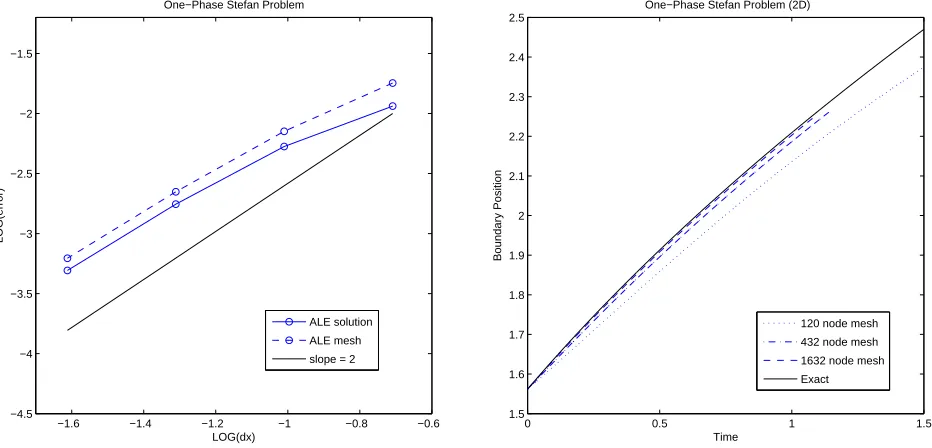
boundary is moving outwards, which represents the freezing of an under-cooled liquid. The results shown in Figure 6 and Table 1 suggest that the method gives an approx-imation which is second order accurate. The evolution of the boundary is shown on the right-hand side of Figure 6, confirming the convergence of the approximation to the exact
solution as the mesh is refined. TimeT = 3 is the point at which the moving inner boundary
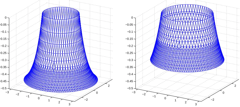
should coincide with the fixed outer boundary. A sample solution profile is shown in Figure 7 which is at a much later experiment time than was possible with the original version of the method presented in [6].
−1.6 −1.4 −1.2 −1 −0.8 −0.6
−4.5 −4 −3.5 −3 −2.5 −2 −1.5
LOG(dx)
LOG(error)
One−Phase Stefan Problem
ALE solution
ALE mesh
slope = 2
0 0.5 1 1.5
1.5 1.6 1.7 1.8 1.9 2 2.1 2.2 2.3 2.4 2.5
Time
Boundary Position
One−Phase Stefan Problem (2D)
120 node mesh
432 node mesh
1632 node mesh
[image:20.612.64.530.214.438.2]Exact
Figure 6: Accuracy of the approximate solutions on a sequence of meshes at T = 0.5 for the
two-dimensional one-phase Stefan problem (left) and the evolution of the average distance of the inner boundary nodes from the centre of the domain (right). The solution and mesh
errors shown are both L2 approximations.
5.2
Two-Phase Results
5.2.1 One dimension
An exact solution to the one-dimensional two-phase Stefan problem is given in [21] as
uS = u
∗
1−erf (x/(2
√
κSt))
erf φ
uL = u0 1−
erfc(x/(2√κLt))
erfc(φpκS/κL)
!
−3 −2
−1 0
1 2
3 −2
0 2 −0.5
−0.45 −0.4 −0.35 −0.3 −0.25 −0.2 −0.15 −0.1 −0.05 0
−3 −2
−1 0
1 2
3 −2
0 2 −0.5
[image:21.612.69.524.18.222.2]−0.45 −0.4 −0.35 −0.3 −0.25 −0.2 −0.15 −0.1 −0.05 0
Figure 7: Snapshots of the solution with the mesh projected on to it for the two-dimensional
one-phase Stefan problem at T = 0 (left) and T = 1 (right).
where φ is the root of the transcendental equation
e−φ2
erf φ+ kL
kS
r
κS
κL
u0e
−κSφ2/κL
u∗erfc(φpκ
S/κL)
+φ λ
√
π KSu∗
= 0, (55)
and erf and erfc are the standard error and complementary error functions, respectively.
The position of the moving interface is given by
s(t) = 2φ√κSt . (56)
In order to compare with previous solutions [28, 33], the parameters are chosen to be
kS = 2.22, kL = 0.556, KS = 1.762, KL = 4.226, λ = 338,
(57)
with u∗
= −20 and u0 = 10, which gives φ ≈ 0.20542692937650. In order to avoid the
singularity at t = 0, the initial time of the experiment is taken at t0 = 0.0012. For this
case a value of δ = 25 was added to the initial and boundary conditions to ensure that the
solution remained positive throughout the domain.
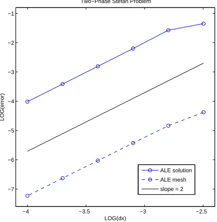
The results shown in Figure 8 and Table 2 (sampled at T = 0.001) clearly show the
method to be second order accurate. Note that, in order to represent the interface accurately, the initial meshes have been adjusted so that half of the total number of mesh cells are in the left-hand region where they are of uniform width. The widths of the remaining cells, in the right-hand region, are calculated using a geometric progression, setting the width of the cell adjacent to the moving interface to be equal to that of its neighbour, on the opposite
side of the interface, and fixing the final node at x= 1.
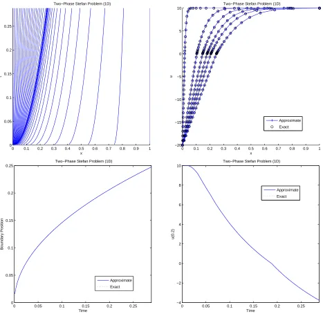
Figure 9 shows a series of results at T = 0.288, which can be compared with those
−4 −3.5 −3 −2.5 −7
−6 −5 −4 −3 −2 −1
LOG(dx)
LOG(error)
Two−Phase Stefan Problem
ALE solution
ALE mesh
[image:22.612.188.404.13.234.2]slope = 2
Figure 8: Comparison of L2 errors in the solution and the magnitudes of the errors in the
boundary node positions for the two-phase Stefan problem in one space dimension.
are considerably more accurate than those presented in [33] but that, due to the explicit time-stepping scheme that is used here, they require significantly smaller (and therefore many more) time-steps to be taken. Figure 10 shows a similar series of results for the same experiment, run until the mesh tangles. The exact and approximate graphs of the boundary
position and the solution at x = 0.2 remain indistinguishable for the whole time (until the
final few time-steps prior to mesh tangling, which are not shown).
Table 2: Numerical estimates of the orders of accuracy of the scheme applied to the two-phase Stefan problem.
Solution errors Mesh errors
L1 L2 L∞
L1 L2 L∞
1D 2.00 2.00 2.01 2.00
Before moving on to the two-dimensional, two-phase case, for which we have no ana-lytic results against which quantitative comparisons may be made, we consider a final one-dimensional example based upon a radially-symmetric problem. This may then be used as the basis for a qualitative assessment of the two-dimensional scheme in the following section. Problem (31) and (32) is solved with initial conditions given by
u(r,0) = (
1−4r2 r ≤ 1
2
1−2r r > 12 (58)
[image:22.612.188.409.470.527.2]0 0.1 0.2 0.3 0.4 0.5 0.6 0.7 0.8 0.9 1 0
0.05 0.1 0.15 0.2 0.25
x
t
Two−Phase Stefan Problem (1D)
0 0.1 0.2 0.3 0.4 0.5 0.6 0.7 0.8 0.9 1 −20
−15 −10 −5 0 5 10
x
u
Two−Phase Stefan Problem (1D)
Approximate
Exact
0 0.05 0.1 0.15 0.2 0.25
0 0.05 0.1 0.15 0.2 0.25
Time
Boundary Position
Two−Phase Stefan Problem (1D)
Approximate
Exact
0 0.05 0.1 0.15 0.2 0.25
−4 −2 0 2 4 6 8 10
Time
u(0.2)
Two−Phase Stefan Problem (1D)
Approximate
[image:23.612.64.531.96.553.2]Exact
Figure 9: Comparison of exact and approximate solutions to the one-dimensional two-phase Stefan problem for a 41 node mesh: node trajectories (top left), snapshots of the solution
0 0.1 0.2 0.3 0.4 0.5 0.6 0.7 0.8 0.9 1 0
0.5 1 1.5 2 2.5
x
t
Two−Phase Stefan Problem (1D)
0 0.1 0.2 0.3 0.4 0.5 0.6 0.7 0.8 0.9 1 −20
−15 −10 −5 0 5 10
x
u
Two−Phase Stefan Problem (1D)
Approximate
Exact
0 0.5 1 1.5 2 2.5
0 0.1 0.2 0.3 0.4 0.5 0.6 0.7 0.8 0.9 1
Time
Boundary Position
Two−Phase Stefan Problem (1D)
Approximate
Exact
0 0.5 1 1.5 2 2.5
−20 −15 −10 −5 0 5 10
Time
u(0.2)
Two−Phase Stefan Problem (1D)
Approximate
[image:24.612.66.530.94.553.2]Exact
Figure 10: Comparison of exact and approximate solutions to the one-dimensional two-phase Stefan problem for a 41 node mesh: node trajectories (top left), snapshots of the solution
surrounded by solid which is held at a fixed temperature (below freezing point, uM = 0) at
the outer boundary: KL = KS = kL = kS = λ = 1 is assumed. The outer boundaries are
treated as Dirichlet boundaries with u=−1 fixed throughout the experiment.
The results obtained for the one-dimensional problem with initial conditions given by (58) are illustrated by Figures 11 and 12. Varying the mesh resolution produces results which are almost indistinguishable: in all cases the peak value in the interior decreases steadily, while the interface initially moves outwards until the point where the gradient of the dependent variable is the same on both sides, after which it starts to move inwards. Note that, as the solution flattens in the inner region, the mesh cells get smaller and eventually (shortly after the final snapshot shown in Figure 11) the mesh tangles and cells with negative lengths appear.
−1 −0.8 −0.6 −0.4 −0.2 0 0.2 0.4 0.6 0.8 1 −1
−0.8 −0.6 −0.4 −0.2 0 0.2 0.4 0.6 0.8 1
x
u
Two−Phase Stefan Problem (1D)
t=0.0 t=0.1 t=0.2 t=0.3 t=0.4 t=0.5
−1 −0.8 −0.6 −0.4 −0.2 0 0.2 0.4 0.6 0.8 1 0
0.05 0.1 0.15 0.2 0.25 0.3 0.35 0.4 0.45 0.5
x
t
[image:25.612.65.532.214.434.2]Two−Phase Stefan Problem (1D)
Figure 11: Evolution of the solutions to the one-dimensional two-phase Stefan problem for a symmetric initial profile and an 81 node mesh: snapshots of the solution profile (left) and node trajectories (right).
A non-symmetric solution is illustrated in Figure 13. The initial conditions were obtained
by shifting the liquid region by 0.25 to the left and assuming linear variation of u in the
remaining solid regions, with the same outer boundary value as before. These results exhibit features that are very similar to those of the symmetric test case.
5.2.2 Two dimensions
0 0.05 0.1 0.15 0.2 0.25 0.3 0.35 0.4 0.45 0.5 0
0.1 0.2 0.3 0.4 0.5 0.6 0.7 0.8 0.9 1
Time
umax
−u
M
Two−Phase Stefan Problem (1D)
21 node mesh
41 node mesh 81 node mesh
0 0.05 0.1 0.15 0.2 0.25 0.3 0.35 0.4 0.45 0.5 0
0.1 0.2 0.3 0.4 0.5 0.6 0.7 0.8 0.9 1
Time
Boundary Position
Two−Phase Stefan Problem (1D)
21 node mesh
41 node mesh
[image:26.612.73.527.37.261.2]81 node mesh
Figure 12: Evolution of the value ofU at the centre of the domain (left) and the position of the
moving interface (right) for the one-dimensional two-phase Stefan problem with symmetric initial profile.
−1 −0.8 −0.6 −0.4 −0.2 0 0.2 0.4 0.6 0.8 1 −1
−0.8 −0.6 −0.4 −0.2 0 0.2 0.4 0.6 0.8 1
x
u
Two−Phase Stefan Problem (1D)
t=0.0 t=0.1 t=0.2 t=0.3 t=0.4 t=0.5
−1 −0.8 −0.6 −0.4 −0.2 0 0.2 0.4 0.6 0.8 1 0
0.05 0.1 0.15 0.2 0.25 0.3 0.35 0.4 0.45 0.5
x
t
Two−Phase Stefan Problem (1D)
[image:26.612.67.532.385.610.2]that the interface moves outwards until the point where the component of the gradient of the dependent variable normal to the interface is the same on both sides, after which it starts to move inwards (see the right-hand side of Figure 15). Figure 15 also illustrates the convergence of the scheme on a succession of meshes for the evolution of the problem up to
t = 0.2. Mesh tangling starts to occur beyondt= 0.21, when the values ofU in the interior
region have all dropped well below 10−4
[image:27.612.68.527.123.565.2]. −1 −0.5 0 0.5 1 −1 −0.5 0 0.5 1 −1 −0.8 −0.6 −0.4 −0.2 0 0.2 0.4 0.6 0.8 1 −1 −0.5 0 0.5 1 −1 −0.5 0 0.5 1 −1 −0.8 −0.6 −0.4 −0.2 0 0.2 0.4 0.6 0.8 1 −1 −0.5 0 0.5 1 −1 −0.5 0 0.5 1 −1 −0.8 −0.6 −0.4 −0.2 0 0.2 0.4 0.6 0.8 1 −1 −0.5 0 0.5 1 −1 −0.5 0 0.5 1 −1 −0.8 −0.6 −0.4 −0.2 0 0.2 0.4 0.6 0.8 1
Figure 14: Solution profiles for the two-phase Stefan results approximating a two-dimensional
radially-symmetric problem at times t = 0.0,0.05,0.1,0.15.
0 0.02 0.04 0.06 0.08 0.1 0.12 0.14 0.16 0.18 0.2 0 0.1 0.2 0.3 0.4 0.5 0.6 0.7 0.8 0.9 1 Time umax −u M
Two−Phase Stefan Problem (2D)
145 node mesh 545 node mesh 2113 node mesh
0 0.02 0.04 0.06 0.08 0.1 0.12 0.14 0.16 0.18 0.2 0 0.1 0.2 0.3 0.4 0.5 0.6 0.7 0.8 0.9 1 Time Boundary Position
Two−Phase Stefan Problem (2D)
[image:28.612.67.530.45.270.2]145 node mesh 545 node mesh 2113 node mesh
Figure 15: Evolution of the value of U at the centre of the domain (left) and the average
distance of the moving interface from the centre of the domain (right) for the two-dimensional two-phase Stefan problem.
−1 −0.5 0 0.5 1 −1 −0.5 0 0.5 1 −1 −0.8 −0.6 −0.4 −0.2 0 0.2 0.4 0.6 0.8 1 −1 −0.5 0 0.5 1 −1 −0.5 0 0.5 1 −1 −0.8 −0.6 −0.4 −0.2 0 0.2 0.4 0.6 0.8 1
Figure 16: Solution profiles for the two-phase Stefan results approximating a two-dimensional
[image:28.612.66.529.410.625.2]6
Discussion
In this paper we have described a generalised form of the multidimensional moving-mesh finite element algorithm introduced in [6] and demonstrated its effectiveness in simulating the solutions of moving boundary problems. The improved robustness and flexibility of the method has been achieved through a series of modifications, which have then been validated on a number of test problems with moving boundaries. These modifications include the abil-ity to impose Dirichlet boundary conditions strongly, the use of an ALE approach to update the solution values (rather than recovering them directly from (4)) and a generalisation of
the way in which the velocity potential (Φ) and rate-of-change of mass ( ˙Θ) are calculated.
However, the method still requires no mesh smoothing.
The generalised method has been described in detail in sections 2 and 2.2, with the algo-rithm given and compared with its predecessor in section 2. Its accuracy and robustness have been illustrated through comparison with analytic solutions of a number of moving boundary problems, in particular a two-phase problem with an internal moving boundary, treated for the first time by this method. The other moving boundary problems studied here include a mass-conserving nonlinear diffusion problem and a non-mass-conserving diffusion problem with a sink term in section 3, and a single-phase Stefan problem included in section 4, both of which have a moving boundary as an implicit part of the solution (both expanding and contracting domains are tested). In all these problems the generalised method successfully reproduces analytic solutions to second order accuracy.
However, the main advance presented in this paper has been the application of the algorithm to multiphase Stefan problems in section 4, involving a weak implementation of the Stefan condition which models the change of phase across a moving interface in the interior of the domain. Comparison with analytic solutions to one-phase and two-phase Stefan problems have demonstrated that the scheme is second order accurate in its approximation of both the solution and the interface position in one and two space dimensions. Further results show that the moving-mesh finite element algorithm can be reliably applied to phase-change problems approximated on genuinely unstructured multidimensional meshes.
The benefits of the strong imposition of the Dirichlet boundary conditions are illustrated
in detail in [29]. However, the solution of (10) and (11) for the velocity potentials Φi and for
˙
Θ, imposing Φ = 0 at one point, and the reliance on the ALE equation do perhaps require further comment. Although the ALE approach appears to yield about the same accuracy as recovering the solution values directly from (4) and both approaches allow conservation of mass to be guaranteed, for some of the test problems considered, such as the two-dimensional two-phase examples, the ALE approach shows significant benefits: without it the solutions obtained can show small non-physical oscillations and the mesh tangles significantly earlier in the simulation. Other approaches to recovering the mesh velocity potentials have been
investigated. In particular, it is possible to construct methods which allow UM = 0 on the
domain, instead of splitting it into its component phases. However, the approach presented here has proved to be the most robust.
As with all moving-mesh methods, there are a number of limitations to the scheme presented here that it is important to discuss. As described, in this work the number of degrees of freedom and the connectivity of the finite element mesh remain fixed throughout each simulation. Clearly this is a restriction that can, and does, lead to mesh tangling when the solution evolves very significantly. Consequently, it makes sense to combine this approach with some form of discrete remeshing that would permit the topology of the mesh to be adapted on occasions. It would of course be important in this approach to address the issue of mass conservation (both local and global) when interpolating between meshes following such an adaptive step.
Another significant constraint on the method, as implemented here, is the explicit time integration scheme that is currently used. This leads to a non-trivial stability restriction on the maximum time-step that may be taken, and thus reduces the overall efficiency of the implementation. This may be overcome by the use of an implicit time-stepping strategy, based upon a multi-step scheme such as BDF2 for example [5], possibly combined with adaptive time-step selection as in [37]. Other generalisations (that are the subject of current work) include the use of different monitor functions to control the mesh evolution and the use of different ALE schemes to update the solution values on the moving grid (see, for example, [8]).
The technique generalises naturally to three-dimensional problems using tetrahedral
meshes and to problems exhibiting features such as blow-up in finite time (see e.g. [16]).
Its capability of simulating multidimensional moving boundary problems and problems with evolving discontinuities suggests that it can be a powerful tool in predicting multidimensional behaviour of nonlinear problems and providing conjectures for further analysis.
Acknowledgements
This work was undertaken with the support of EPSRC Grant EP/D058791/1. R. Mahmood wishes to thank his employer PINSTECH for granting him study leave to carry out research work at Leeds.
References
[1] R.Almgren, Variational algorithms and pattern formation in dendritic solidification,J.
Comput. Phys., 106:337–354, 1993.
[2] B.N.Azarenok and T.Tang, Second-order Godunov-type scheme for reactive flow
[3] D.G.Aronson, The Porous Medium Equation, inLecture Notes in Mathematics,1224:1– 46, 1986.
[4] M.J.Baines, Moving finite elements, Oxford University Press, 1994.
[5] K.W.Blake and M.J.Baines, Moving-mesh methods for nonlinear partial differential equations, Numerical Analysis Report 7/01, Department of Mathematics, University of Reading, UK, 2001.
[6] M.J.Baines, M.E.Hubbard and P.K.Jimack, A moving mesh finite element algorithm for the adaptive solution of time-dependent partial differential equations with moving
boundaries, Appl. Numer. Math., 54:450–469, 2005.
[7] M.J.Baines, M.E.Hubbard and P.K.Jimack, A moving mesh finite element algorithm
for fluid flow problems with moving boundaries, Int. J. Numer. Methods Fluids,
47(10/11):1077–1083, 2005.
[8] M.J.Baines, M.E.Hubbard, P.K.Jimack and A.C.Jones, Scale-invariant moving finite
elements for nonlinear partial differential equations in two dimensions, Appl. Numer.
Math., 56:230–252, 2006.
[9] G.I.Barenblatt, Scaling, Cambridge University Press, 2003.
[10] G.Beckett, J.A.Mackenzie and M.L.Robertson, A moving-mesh finite element method
for the solution of two-dimensional Stefan problems, J. Comput. Phys., 168:500–518,
2001.
[11] A.E.Berger, M.Ciment and J.C.W.Rogers, Numerical solution of a diffusion
consump-tion problem with a free boundary, SIAM J. Numer. Anal., 12:646–672, 1975.
[12] P.Bochev, G.Liao and G.dela Pena, Analysis and computation of adaptive moving grids
by deformation, Numer. Meth. Part. D. E.,12:489–506, 1998.
[13] C.Bonacina, G.Comini, A.Fasano and M.Primicerio, Numerical solution of phase-change
problems, Int. J. Heat Mass Tran., 16:1825–1832, 1973.
[14] C.J.Budd, G.J.Collins, W.Z.Huang and R.D.Russell, Self-similar numerical solutions
of the porous-medium equation using moving mesh methods, Philos. T. Roy. Soc. A,
357:1047–1078, 1999.
[15] C.J.Budd and M.D.Piggott, Geometric integration and its applications, Foundations of Computational Mathematics, Handbook of Numerical Analysis XI, ed. P.G.Ciarlet and F.Cucker, Elsevier, pp. 35–139, 2003.
[16] C.J.Budd and J.F.Williams, Parabolic Monge-Amp`ere methods for blow-up problems
[17] W.M.Cao, W.Z.Huang and R.D.Russell, An r-adaptive finite element method based
upon moving mesh PDEs, J. Comput. Phys.,149:221–244, 1999.
[18] W.M.Cao, W.Z.Huang and R.D.Russell, A moving-mesh method based on the geometric
conservation law, SIAM J. Sci. Comput., 24:118–142, 2002.
[19] N.N.Carlson and K.Miller, Design and application of a gradient-weighted moving finite
code I: In one dimension, SIAM J. Sci. Comput., 19:728–765, 1998.
[20] N.N.Carlson and K.Miller, Design and application of a gradient-weighted moving finite
code II: In two dimensions, SIAM J. Sci. Comput.,19:766–798, 1998.
[21] H.S.Carslaw and J.C.Jaeger, Conduction of Heat in Solids, Oxford University Press,
1959.
[22] S.Chen, B.Merriman, S.Osher and P.Smereka, A simple level set method for solving
Stefan problems, J. Comput. Phys., 135:8–29, 1997.
[23] J.Crank, Free and Moving Boundary Problems, Oxford University Press, 1984.
[24] J.Crank and R.S.Gupta, A moving boundary problem arising from the diffusion of
oxygen in absorbing tissue, J. Inst. Math. Appl., 10:19–33, 1972.
[25] Y.Di, R.Li and T.Tang, A general moving mesh framework in 3D and its application
for simulating the mixture of multi-phase flows, Commun. Comput. Phys., 3:582–602,
2008.
[26] M.J.Djomehri and J.H.George, Application of the moving finite element method to
moving boundary Stefan problems, Comput. Method. Appl. M., 71:125–136, 1988.
[27] F.C.Frank, Radially symmetric phase growth controlled by diffusion, Proc. R. Soc. A,
201:586–599, 1950.
[28] R.M.Furzeland, A comparative study of numerical methods for moving boundary value
problems, J. Inst. Math. Appl.,26: 411–429, 1980.
[29] M.E.Hubbard, M.J.Baines and P.K.Jimack, Mass-conserving Dirichlet boundary
conditions for a moving mesh finite element algorithm, Appl. Numer. Math.
doi:10.1016/j.apnum.2008.08.002, 2008.
[30] W.Z.Huang and R.D.Russell, Adaptive mesh movement – the MMPDE approach and
its applications, J. Comput. Appl. Math., 128:383–398, 2001.
[31] W.Z.Huang and X.Y.Zhan, Adaptive moving mesh modeling for two dimensional
groundwater flow and transport, In AMS Contemporary Mathematics, 383:283–296,
[32] R.Li, T.Tang, and P.Zhang, A moving mesh finite element algorithm for singular
prob-lems in two and three space dimensions, J. Comput. Phys., 177:365–393, 2002.
[33] J.A.Mackenzie and M.L.Robertson, The numerical solution of one-dimensional
phase-change problems using an adaptive moving-mesh method, J. Comput. Phys., 161:537–
557, 2000.
[34] K.Miller and R.N.Miller, Moving finite elements I, SIAM J. Numer. Anal., 18:1019–
1032, 1981.
[35] J.D.Murray, Mathematical Biology: An Introduction(3rd edition), Springer, 2002.
[36] J.Ockendon, The role of the Crank-Gupta model in the theory of free and moving
boundary problems, Adv. Comp. Math.,6:281–293, 1996.
[37] J.Rosam, P.K.Jimack and A.M.Mullis, A fully implicit, fully adaptive time and space
discretization method for phase-field simulation of binary alloy solidification,J. Comput.
Phys., 225:1271–1287, 2007.
[38] T.Tang, Moving mesh methods for computational fluid dynamics, In AMS
Contempo-rary Mathematics, 383:141–173, 2005.
[39] Z.-J.Tang, T.Tang and Z.R.Zhang, A simple moving mesh method for one- and
two-dimensional phase-field equations J. Comput. Appl. Math., 190:252–269, 2006.
[40] P.D.Thomas and C.K.Lombard, The geometric conservation law and its application to
flow computations on moving grids, AIAA J., 17:1030–1037, 1979.
[41] J.L.Vazquez, The Porous Medium Equation: Mathematical Theory, Oxford University
Press, 2006.
[42] B.V.Wells, A moving mesh finite element method for the numerical solution of partial differential equations and systems, PhD thesis, Department of Mathematics, University of Reading, UK, 2005.
[43] B.V.Wells, M.J.Baines and P.Glaister, Generation of Arbitrary Lagrangian-Eulerian (ALE) velocities, based on monitor functions, for the solution of compressible fluid
equations, Int. J. Numer. Methods Fluids,47(10/11):1375–1381, 2005.
[44] P.A.Zegeling, W.de Boer and H.Tang, Robust and efficient adaptive moving mesh
so-lution of the 2-D Euler equations, In AMS Contemporary Mathematics, 383:419–430,