THE EVOLUTION OF HII REGIONS IN THE LARGE MAGELLANIC CLOUD
I.R.G. WILSON 1983
This thesis is dedicated to my father,
Ian Andrew Wilson and mother, Marion Noreen Wilson, whose love and sacrifice have made
The work described in this thesis is
that of the candidate alone, except where noted otherwise in the text.
February 1983
iv
ACKNOWLEDGEMENTS
Any large project is only made possible through the contribution and help of many people. First and foremost among those I would like to thank is my supervisor, Dr. Michael Dopita, who was responsible for the original idea on which this thesis was based. His encouragement, enthusiasm and ideas were provided at times when they were most needed.
I would also like to thank Dr. Alex Rodgers who patiently answered my various questions and showed up at the oddest hours to see how I was going.
Thanks also goes to the other staff members and students at Stromlo for providing a friendly and inform ative environment in which to work.
The observations in this thesis required the close support of the electronics, mechanical and optical staff at Mr. Stromlo Observatory, and the technical staff at the Siding Spring Observatory. Special thanks goes to David Irons and Bob Moon who both managed to maintain their sanity in the face of the trials I presented them with. I would also like to thank the night assistants for the competent help they provided for the observations on the 74 inch telescope.
V
Staff for their friendly assistance throughout my stay at M t . Stromlo. Special thanks goes to Su Khouri and Maria Sharr for typing all sorts of odds and ends for me.
There have been a number of people who have contributed to the final compilation of this thesis. I am grateful to A n d r e w Pickles who was responsible for the final collation of this thesis and who, on m a n y occasions aided me with my computing problems, and to Dr. Marshall McCall for proof reading the manuscript.
I would also like to thank Sue Parkes who aided with the diagrams, Keith Smith who did the photography and Andrew Kulessa who was always willing to help with the thesis work* and ready to discuss the trials and tribulations of writing a thesis.
I am deeply grateful to the people at the Reid Uniting Church for their Christian fellowship and
spiritual guidance. There are many I would like to thank but cannot here because I would push this t h e s i s over the 100,000 word limit. I would like to give
special thanks to Paul Bainton, Mark Sterland, Rev. Keith Doust, Don and Annette Purdy and Doug, June, Mark, Tim and A l e x a n d r a Faulkner.
vi ABSTRACT
A study of the effect of mass-loss from OB stars upon the evolution of HII regions in the Large Magellanic Cloud is presented. This study incorporates spectra- scopic observations of 25 OB stars in 10 clusters located within L.M.C. HII regions, together with narrow band
hydrogen-alpha surface photometry of an overlapping sample of 15 HII regions.
Empirical calibrations based on prior studies of Galactic OB stars are used to determine the integrated
stellar wind mechanical luminosity (L^) and the integrated Lyman continuum photon luminosity (S*) of the 10 OB clusters.
The ratio between the momentum carried away from a star by the stellar wind to the momentum carried away by photons is found to be 0.7±_0.3, for OB stars with log M ^-6.3. This fact, together with the scaling law that is found between the stellar wind terminal velocity and the stellar escape velocity, is used to empirically relate the mass-loss rate of an OB star to its luminosity, radius and mass. The dependence of M on the stellar parameters found is not predicted by the line-driven wind or Fluctuation theories for mass-loss,
indicating that these theories;must be modified in order to remain viable.
S+, L M and the stellar wind momentum transfer rates * w
vii
core-hydrogen burning lifetimes for stars with initial masses of 20,30,40,50,60,80 and 100 M • These
calcula-e
tions show that the magnitudes of and S* are essentially constant during this phase of evolution, and that they
are primarily dependent on the initial mass of the OB star.
These calculations also show that at the beginning of core-hydrogen burning, the ratio L^/S* has a constant value equal to 3.2^0.4 xlO-^ (Joules photon for 20 to 100 M stars.
A comparison of the integrated values of S* for the L.M.C. OB clusters with the ionizing photon absorption rate of the surrounding nebulae, via the Zanstra method, shows that the L.M.C. HII regions are in general ionization bounded.
The values of L and S* for the L.M.C. OB clusters,
w *
together with the hydrogen-alpha surface photometry, are used to show that the large shell-like HII regions in the L.M.C. are stellar wind bubbles 3 to 5 million years old. In order to reproduce the observed densities in the shells of these HII regions a thick cushion of shocked stellar-wind gas must have been present on the inside of the HII shell for most of the lifetime of the nebula. The stellar wind mechanical luminosity, the age of the central clusters and the radius of the HII shells indicate that the stellar wind bubbles are moving into an I.S.M. with a typical time
7 -3
viii
high are typical of those found in the outer parts of large massive molecular clouds. This raises the possibility that
the HII regions are being ram pressure confined by the infalling gas in the molecular cloud.
TABLE OF CONTENTS ix
Acknowledgements Abstract
List of figures List of Tables
CHAPTER 1 CHAPTER 2
2.1 2.2 2.3 2.4
INTRODUCTION
THE EVOLUTION OF Mil REGIONS
Evolved Mil Regions - The Classical Model The Blister Model
Stellar Wind Bubbles
The Off-centre Accretion Model
iv vi xiii xiv 1 6 8 9 20
CHAPTER 3
-3.1 3.2
SPECTRAL CLASSIFICATION OF 0 AND B STARS IN THE L.M.C.
The M.K. Spectral Classification System The Adopted Method of Spectral Classi fication for O and B Stars
24 24
3.2.1 0 Stars 27
3.2.2 Luminosity Indicators for 0 Stars 27
3.2.3 09 to B5 Stars 29
3.2.4 The Luminosity Class of L.M.C.
31 OB Stars
3.2.5 Luminosity Indicators for BO to B5
Stars 32
3.2.6 The Spectral Classification ocheme 33
3.3 The Observations of L.M.C. OB Stars 3.3.1 Constraints on the Observations 3.3.2 The Observations
3.3.3 The Reduction Procedure
35 35 37 41
3.4 The Spectral Types of L.M.C. OB Stars 43
43 3.4.1 Spectral Types
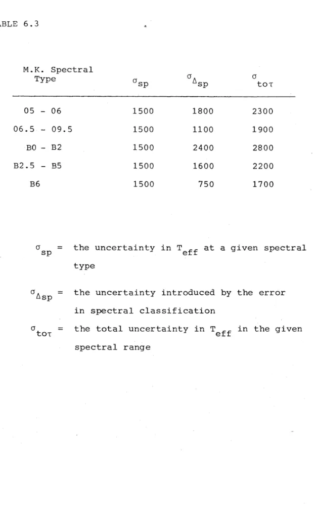
3.4.2 Uncertainties in the Classification Procedure
PAGE
CHAPTER 4 THE INTEGRATED LYMAN CONTINUUM PHOTON FLUX
OF L.M.C. OB CLUSTERS 46
4.1 4.2 4.3
4.4
Introduction
Theoretical Atmospheric Models for OB Stars The Lyman Photon Flux (S ) as a Function of
L M.K. Spectral Type
Results for L.M.C. Stars
46 47
50 57 CHAPTER 5
5.1 5.2
5.3
5.4
MASS-LOSS IN OB STARS Introduction
Methods for Determining Mass-Loss Rates for OB Stars
5.2.1 Mass-Loss Rates Derived from U.V. Resonance Lines
5.2.2 Mass-Loss Rates Derived from Radio Observations
5.2.3 Mass-Loss Rates Derived from Infra- Red Observations
5.2.4 Mass-Loss Rates Derived from Hydrogen Alpha Emission
The Adopted Sample of Mass-Loss Rates 5.3.1 Lamers Sample of Mass-Loss Rates
5.3.2 Modifications to the Sample of Lamers The Mass-Loss Rate as a Function of Stellar Parameters
5.4.1 M as a Function of L* 5.4.2 Et a L*
5.4.3 E a (t /t )** L*
T D K
5.4.4. Em /T7 / \ — T - (Vesc/c) L*
xi
PAGE
CHAPTER 6
6.1 Introduction 92
6.2 The Effective Temperature Scale for
94 OB Stars
6.3 Evolutionary Models for OB Stars 100
6.4 Results of the Evolutionary Models 102
6.5 Conclusions 105
6.5.1 The Distinction between Of and non Of Stars in the Adopted
Sample 105
6.5.2 The Transition of Of Stars
to W-R Stars 107
6.5.3 The Denisty of the Stellar
Wind Envelope 109
6.6 The LMC HII Regions H 0
6.6.1 Results H O
6.6.2 Discussion and Conclusions H 2
CHAPTER 7 - SURFACE PHOTOMETRY AND CONCLUSIONS
7.1 The Instrumentation H 5
7.1.1 The S.E.C. Vidicon T.V. 2 -D Photometer H 5
7.1.2 The Optics H 7
7.1.3 The Hydrogen Alpha Filter H ®
7.2 The Method of Observation H 9
7.3 The Initial Reduction Procedure 122
124 7.4 The Integrated Ha- Flux
7.5 The Surface Brightness of the L.M.C. HII
Regions 128
X l l
7.6.1 Are the HII Regions Ionization or Density Bounded?
7.6.2 The Hot Cushion and Direct Impingement Models
REFERENCES
PAGE
131
137
List of figures
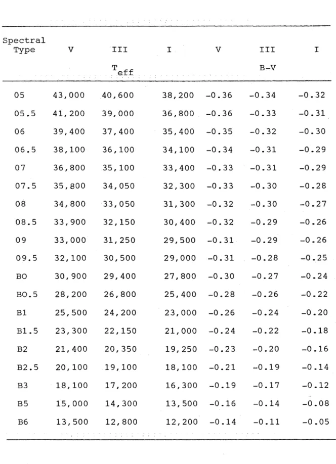
3.1 The apparent visual magnitude and absolute visual magnitude as a function of MK
spectral type.
4.1 Log Fl as a function of stellar effective temperature.
4.2 Log (N /ttF ^ as a function of MK spectral type for dwarf stars.
5.1 Log M as a function of Log (L /L ) for all stars in the adopted sample.
5.2 Log M as a function of Log (L*/L@) for supergiant stars.
5.3 Log M as a function of Log (L*/L@) for non-supergiant stars.
. 2
5.4 Log M as a function of Log ( (L*/L@)/Vesc ). 5.5 Log M plotted against the Andriesse formula
for mass loss.
5.6 Log M as a function of Log ((L*/L@)/V ). 5.7 Log M as a function of Log ( (L*/L@)/V esc ) . 6.1 The effective temperature scale as a function
of the MK spectral type for 04 to B3 stars. 6.2 The parameters a) Log M; b) Log L ;
c) Log MV^ and d) Log Lw as functions of
stellar age for various initial stellar masses. 6.3 HR diagram for OB stars in the adopted sample. 6.4 Actual and minimum (necessary to expose
enriched core material) percentages of mass loss as a function of stellar initial mass. 6.5 Log M as a function of Log ( ^ R * 2).
7.1 The optical train for the TV photometer-Reducer combination.
7.2 Transmission profile for the Ha filter used for the HII region observations.
7.3 Rate at which LMC HII regions absorb ionizing photons (Zanstra method) as a function of the ionizing stellar emission rate.
7.4 Dereddened, integrated H a flux as a function of HII region diameter.
7.5 Integrated H a flux (derived from stellar Lyman continuum) as a function of HII region diameter.
7.6 Log (t L ) as a function of HII region radius.
6 w
L w for LMC HII regions as a function of their r adi i *
xiv 7.8 Lyman continuum photon luminosity (S*) and
stellar wind mechanical luminosity (L ) as a function of initial stellar mass.
7.9 (a to m) Absolute Ha surface brighteness maps for 13 LMC HII regions.
143
145
X V
List of tables
3.1 MK spectral type for 0 stars based on the W(4471)/W(4542) Ratio VT .
3.2 Spectral discriminants for 09 to B5 spectra at MK dispersion.
3.3 Standard stars : 09 - B5.
3.4 Summary of spectral observations.
3.5 LMC HII region bright stars : parameters. 3.6 LMC HII region bright stars : equiv. widths. 4.1 Adopted relationship between Log (N /ttF )
and MK spectral type. L v
4.2 LMC HII regions : physical parameters. 5.1 Mass Loss rates : stellar sample.
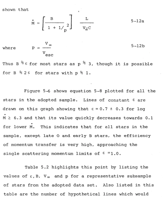
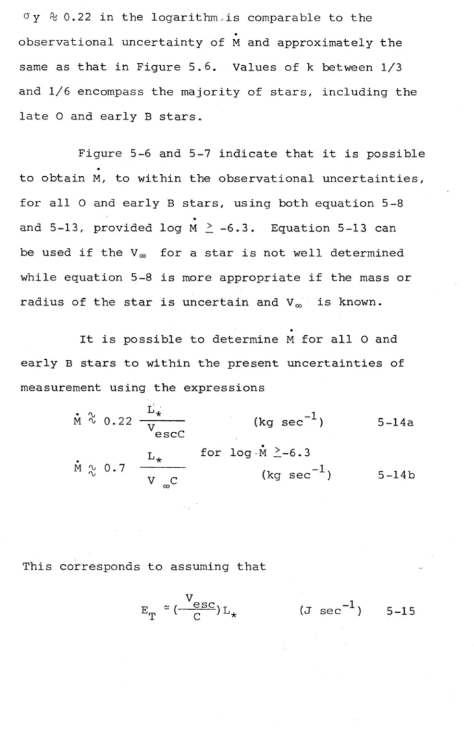
5.2 Table of e , B, V and p for a representative
subsample of stars from the adopted data-set. 6.1 Adopted temperature scale.
6.2 LMC HII region stars : a) astronomical parameters; b) physical parameters.
6.3 Calculated errors due to uncertainties in Teff and spectral type.
7.1 Ha Surface photometry observation summary. 7.2 Surface photometry flat-fields.
7.3 Surface photometry reduction summary.
7.4 Surface photometry; extinction determinations. 7.5 Surface photometry; standard observations. 7.6 Surface photometry; conversion factors. 7.7 LMC HII regions; electron densities. 7.8 LMC HII region stellar wind parameters. 7.9 LMC HII region densities.
Details of Ha surface brighteness maps (figures 7.9 a to m ) .
CHAPTER 1
Introduction
The aim of this thesis is to investigate the evolution of HII regions in the large Magellanic Cloud
(L.M.C.) through a combined study of the regions and the young OB stars embedded within them.
The L.M.C. was chosen as it is the closest ex
ternal galaxy to our own, providing us with the opportunity to observe a large number of relatively unobscured HII
regions of widely differing morphology and known distance. These properties, proximity and low reddening, are also advantageous for observing the individual OB stars located within the HII regions. It was not until the advent of high
sensitivity photon counting detectors though, that a thesis of this nature became viable. Using these modern detectors it is possible to obtain high signal to noise, moderate
( ~lOOA/mm) dispersion spectra of bright LMC OB stars in less than 30 minutes.
The HII regions chosen for this study were selected on the basis that they were relatively free of obscuration; that they have a relatively simple geometry with near
spherical symmetry; and that they have less than roughly a dozen bright OB stars located within them. The last two criteria selected against the high surface brightness
large HII regions which have tens and sometimes hundreds of OB stars located within them. The choice of simple mor phology and spherically symmetric structure was stipulated to minimize complications due to density inhomogenities in the ISM. The catalogue of L.M.C. HII regions published by Henize (1956) showed that the L.M.C. has many HII
2
star formation located at the Eastern end of the stellar bar. The other HII regions are either associated with weak spiral arm features, or are found in irregular
scattered regions of star formation which cover areas of the order of a kiloparsec. (Meaburn 1979,80)
A more recent catalogue of L.M.C. HII regions is that of Davies, Elliott and Meaburn (1977) (D.E.M.), and is based on deep UK Schmidt Telescope plates taken in con junction with a mosaic H ot filter. This catalogue includes information on the position, size and brightness of over 300 HII regions, and penetrates to a fainter surface bright ness than that of the Henize catalogue thus giving a clearer and more comprehensive picture of the distribution of L.m .C. HII regions. The nomenclature used in the catalogue of
Davies et. a l . has been used in this thesis.
The corresponding Henize number of each HII region can be found in this catalogue.
3
presence of shock phenomena. (Lasker, 1979 , 1981). The shell-like morphology and the fact that the radio fluxes of these nebulae roughly fit on the Z-D relation for L.M.C. supernovae (Milne e t . al. 1980) have led various authors to speculate that they are evolved supernova remenants. Evidence which contradicts this hypothesis includes measured
4
electron temperatures of - 10 K (Lasker 1981, Dopita et. al. 1982), the presence of thermal radio spectra in D.E.M. 301 (N70), (Dopita et. a l . 1982) and in D.E.M. 192
(N51D) (McGee and Newton 1972) and D.E.M. 241 (N59A)
(Meaburn et. al. 1981), and the presence of OB stars within the HII shells. These have led some people to speculate that these large HII rings are stellar wind bubbles
(Meaburn 1978, Meaburn and Blades 1980 and Lasker 1980) formed from the mass-loss from the OB stars. The problem with these objects is that neither the supernova hypothesis nor the classical stellar wind bubble hypothesis can explain all the observational characteristics of those nebulae.
The observations of the dynamics of the ionized gas in these nebula have been so far unable to resolve this dilemma. The velocity fields of nebulae such as D.E.M. 301
(Rosado e t . a l . 1981, Blades e t . al. 1980, Dopita et. a l . 1982), D25 (Rosado et. al . 1982), D192 (Lasker 1980, Meaburn and Terrett, 1980, Klaus de Boer and Nash 1981), D241
4
expanding shell. A number of different hypotheses have been proposed to describe the- velocity structure of these nebulae. Lasker (1980) adopted a stellar wind bubble model evolving into an inhomogenous I.S.M. to fit the velocity structure of D.E.M. 192. Meaburn and Terrett (1980) and Meaburn et.al. (1981) used a model which has an expanding
shell, formed by energetic stellar winds or multiple super nova explosions, expanding into an I.S.M. consisting of large sheets of neutral hydrogen. On the other hand Rosado e t . al.
(1981,1982) preferred a supernova explanation for D301 and D25 to describe the velocity structure of these nebulae.
Dopita (1981) proposed a third model in order to try to explain the confusing observational picture which has developed for the L.M.C. HII rings. Dopita's model has a stellar wind bubble being formed by mass-loss from an OB star (or stars) located off-centre in a large collapsing
molecular cloud. The stellar wind bubble quickly establishes a quasi-static configuration where the ram-pressure of the stellar wind just balances the corresponding rampressure of the infalling cloud material. This model was applied to D.E.M. 301 and it was able to produce all of the major ob servational characteristics of this nebula including the velocity structure. (Dopita e t . a l . 1982) .
5
the models proposed above (if any) apply to the L.M.C. HII
r egions.
In the following chapter (Chapter 2) the various
models which are applicable to evolved HII regions are
discussed. This work clearly shows the need to know the
ionizing photon luminosity and mass-loss rates (M) for the
OB stars embedded in the L.M.C. HII regions.
In Chapter 3 the M.K. spectral types are determined
for the bright OB stars located within the L.M.C.HII regions.
Chapter 4 indicates the method which was adopted to determine
the integrated Lyman continuum photon flux for the L.M.C.
OB clusters, using the M.K. Spectral types derived in
Chapter 3. Chapter 5 discusses the various relationships
between the mass-loss rates of OB stars and their gross
properties, i.e. luminosity (L*), radius (R*) and mass (M*).
The relationship between M and L ., R* and M + , . , . ,
^ * * * which is adopted
in this chapter has been used in Chapter 6 to determine the
2
integrated stellar wind mechanical luminosity (J^MV <» ) and
momentum transfer rate (MV^ ) for the L.M.C. OB clusters
(V^ is the terminal velocity of the stellar w i n d ) .
In the final chapter of this thesis, integrated H a
fluxes and surface brightness contour maps of the L.M.C. HII
regions are presented. These data enable the integrated
stellar parameters of the OB clusters derived in Chapters
3 and 6, to be compared with the properties of the HII regions.
This final chapter ends with the discussion and conclusions
CHAPTER 2
6
2. THE EVOLUTION OF HII REGIONS
2.1 Evolved HII Regions - The Classical Model
The evolution of a HII region in a uniform low density medium is reasonably well understood (Lasker
1967, Mathews and O'Dell 1969), being characterised by the following features. Soon after the ionizing star
(or stars in the case of an OB association) is formed, an R-type ionization front propagates supersonically into the surrounding I.S.M. The R-front continues to expand supersonically until a point is reached where
all the available ionizing photons from the star are used up in maintaining the HII region. The radius at which this occurs is designated as the Initial Stromgren Radius R , given by the expression
( 3 L
uv )
1/3
s a 2
(4TT n n
02
)
2 -1
where L^v is the number of photons/sec emitted by the star, n^j. is the HII region electron density and olz is
the recombination coefficient for the excited levels of hydrogen. (Stromgren 1939).
Once the Initial Stromgren Sphere is formed the ionization front (I front) becomes a weak D-type front with an isothermal shock preceeding it. This shock
7
establishment of the initial Stromgren Sphere, provides the driving force for this shock and so the weak D-type front will continue to expand until pressure equilibrium is established.
the expansion phase is equal to that in the undisturbed I.S.M. The expansion is communicated to the HII region via a rarefaction wave which propagates sonically
into the ionized gas. At later phases, when the sound crossing time scale is short compared to the evolutionary timescale, then the density within the HII region is
once again constant, and the constant ionizing flux from the central star is given by
The density of the HII region at the start of
3/2
2 -2
where p is the density in the I.S.M., p TT is the
o I-L
o
density of the HII region and R is the radius. R is given by the expression
r t
7 L II 4/7 R / R = ( 1 + - --- )
4 R 2-3
s
s
Spitzer (1978).
8
shell-like structures. It is difficult to imagine how the classical picture discussed above could produce those large shell-like HII regions. At best, the morphology of an evolved HII region would appear as a
relatively low density HII region with a very sharp boundary making the ionization front. This model
would certainly not produce the large relatively thick shells observed in the L.M.C. HII regions.
2.2 The Blister Model
An alternative theory which appears to fit most of the observations characteristics of Galactic HII regions (Osterbrock 1974, Tenario-Teagle 1978) is the Champagne (or Blister) Model. This model embraces the fact that regions of active star formation usually take place near large ( -60-80 pc) molecular clouds of mass
104 to 105 M0 , invalidating the uniform density
approximation of the classical theory. In brief outline the evolution described by this model is as follows.
The Champagne model assumes that an ionizing
star (or stars in the case of an OB association) switches on near the edge of a large dense molucular cloud and begins to form an Initial Strbmgren Sphere. Eventually the I-front breaches the outer boundary of the cloud and rushes into the low density inter-cloud medium
9
ionized cloud material and the ionized I.C.M. results in a strong shock forming at the breach in the
molecular cloud boundary. The shock then propagates supersonically into the ionized I.C.M. followed by the ionized cloud gas. The expansion of the HII region out through the breach in the cloud results in the
progation of a rarefaction wave back into the cloud HII region, towards the ionizing stars. This wave decreases
the density of the molecular cloud HII region to that of the HII region which is expanding into the I.C.M.
Although this model can reproduce the assymetric blister type HII regions such as the Orion nebula,
it does not produce shell structures in the ionized gas. In order to produce these structures we have to consider the effects of stellar winds from the massive OB stars upon the HII region.
2.3 Stellar Wind Bubbles
Models for expanding spherically symmetric
stellar wind bubbles have been discussed extensively by Pikel'ner and Shcheglor 1969, Avedisova 1972 , Dyson and deVries 1972, Falle 1975 and Weaver et. al. 1977. The following discussion outlines the major character istics of these bubbles as outlined by Weaver et. al. An evolved stellar wind bubble can be subdivided into
10
is the freely expanding hypersonic wind (zone 1). This stellar wind sweeps up a shell of shocked interstellar gas (or ionized gas if the bubble is expanding into an HII region). The collision of the wind with this shell sets up a reverse "bow" shock in the stellar wind flow
> c
which forms the second zone of hot (~10 K) shocked gas behind the dense shell. The third zone is the shocked interstellar gas (or ionized gas) which forms behind the isothermal shock produced by the piston action of
zone 2. Zones 2 and 3 are separated by a contact
discontinuity across which a conduction front develops due to the large temperature difference between the two zones. The final zone (zone 4) is the surrounding
ambient I.S.M. (or ambient HII region) into which the shell propagates.
The evolutionary history of a stellar wind
bubble consist of three stages. In the short formative stage (Falle 1975) the bubble is expanding so fast
that the radiative losses in the gas do not have time to affect the gas dynamics of the flow. The second stage begins when the radiative losses in the swept up inter stellar gas cause it to collapse into a thin shell. The radiative cooling in the shocked stellar wind is not significant in this stage because of the low density of the material. The major cooling mechanism in this region is by heat conduction across the contact
11
the cool shell material across this conduction front provides the major source of mass increase in region 2.
The final evolutionary stage begins when the radiative cooling becomes important in zone 2, leading to the
collapse of this region and allowing the stellar wind to directly impinge on the outer shell. In the following discussion we will only be concerned with the last two stages of the evolution of a stellar wind bubble.
If the radiative losses in zone 2 are ignored Castor et. al. (1975) showed that the radius R(t) and the velocity V(t) of the outer isothermal shock is given by
and
R (t) s
V (t) s
427.9 L 291/5 n o 1/5 t 63/5
(pc) 2-4
253.6 L 291/5 » o ' 175 t 6
(km/sec) 2-5
where L 29 (-^ M V ^ 2) i-s mechanical wind luminosity
in units of 1.0 x 10 29 J sec \ n o is the ambient I.S.M. _3
density in particles m and t6 is the nebula age in 106 years.
12
input from the stellar w ind the zone will collapse and the stellar wind will impinge d i rectly onto the outer shell. In this case the time dependence of shell
radius (R ) will f o l l o w the formula given by Steigman
O i l
e t . al. (1975).
i . e .
(3 Mv
y
4 t ^OO
4tt p 0
(m) 2-6
with shell having thickness
AR/R
(-P o C II
■) R
3 MV SH
2-7 According to We a v e r e t . al. (1977) never exceeds
because of a re g u l a t o r y m e c h a n i s m which governs the losses in zone 2. T h e y cla i m that if radiative cooling sets in, it will lead to a reduction in the mass flux into zone 2 from the HII shell. The decrease in mass flux across the front causes the density in zone 2 to decrease in such a way as to limit any further increase
in the cooling.
This p i c ture is c omplicated t h ough if we consider situations in which the stellar wind bubble is not
spherically symmetric. In this case there will be strong streaming moti o n s in the shock stellar wind m a t e r i a l
13
Kahn (1980) showed that the interface between the stream ing stellar wind bubble and the HII shell, is subject to Kelvin-Helmholtz instability. He also showed that while turbulent mixing is produced by the instabilities,
it is limited until the shocked stream has lost most of the thermal energy that it gained in the shock. Kahn finds that the shocked gas would have to cool to roughly
5
3x10 K before the shock layer would be destroyed by turbulent mixing. Thus it is possible the hot cushion of gas in zone 2 could be destroyed at some point during the evolution of the nebula. Without a detailed
theoretical model to determine the point at which this occurs, all that we can do is consider the two extreme conditions i.e. the case where zone 2 does not collapse
(the hot cushion model) and the case where it does (the direct impingement model). In the following discussion on stellar wind bubbles, both models will be discussed. Due to the fact that ionizing stars within HII regions are also the major source of stellar wind mechanical energy, it is almost certain that the majority of the stellar wind bubbles will begin their evolution within a HII region. In order to gauge the effect this stellar wind bubble would have upon the HII region a number of
important time scales need to be considered.
14
S i ‘ “ 4ttRSH aR“ 2 n SH 2-8
where AR, R a n d n_ u are the shell thickness, radius
on on
and density respectively.
If the shell were to continue increasing in mass
it would eventually absorb all of the photons emitted
by the star and the I-front would be trapped. The
condition for trapping of the I-front is given by
S . ' = L . The radius at which this event occurs can be
1 uv
determined from the Rankine-Hugoniot conditions, which
across the outer isothermal shock give:
U + (
v sh/
cti)
)
2-9
Combining this with equations 2.1 and 2.8 we have
— = 3(AR/RSH> (1 + (VSH/CI I )2)~ 1/3 2-10
Rs
Now equation 2-10 can be used along with the equations
2-4 and 2.5 describing (VotJ/ C TX ) at the point when the
I-front is trapped. In the case of the hot-cushion
model, (HC model) this is given by the transcendental
equation
(1 + (VSH/CII)2 = 399.31 (1/(3aR / R ch) ) S b n 48 L 29 J--L ‘/2
9 / 2 x ( V cu/C )
15
where S^g is the ionizing photon flux in units of 10
photons sec ^ and = 11.77 km/sec (the isothermal
4
sound speed at a T g of 10 K ) . In the case of the direct
impingement model (DI model) the corresponding relationship
is
(1
+ (
v sh/Cxi)2)
= 1-0331 x 105 (1/(3Ü R / R SH) ) sw M23 3 /2 1/2X
(v s h/c x i>3 2-12
where M^^is the momentum deposition rate by the stellar
wind onto the HII shell, in units of 1.0 x 1C?^ Newtons.
If we take values of S^g= 40.0, Lg g= 13.0 and
M
23 = 5.0, typical for a small OB association (see
ß
Chapter 6) and assume that aR / Ro u = 0-2 and n = 10
o r i -L
particles m -^, we find that (V___/C__) ~ 1.46 for the HC
on 1 1
model and 0.12 for the DI model. These velocities correspond
to the I front being trapped at R.^/R-. ~ 0.81 and 1.8
bH o
respectively. The stellar wind bubble will reach this
radius after 3.0 million years in the case of the HC
model and 44.7 million years for the DI model. Clearly,
for the assumed outer HII region density, the DI stellar wind
shell will not trap the ionization front before it stalls.
The HC stellar wind shell on the other hand, will trap
16
If we take ^ C which is the condition which defines the period in which the bubble has not
stalled, then we find from equations 2-11 and 2-12 that the constraint for trapping the I front prior to stalling is
n
II > 2.26337 x 10⁴
- (3Ar/rsh)2
2-13
for the HC model, and
n
II > 2.66823 x 10⁹ (3AR/RSH) 2
2-14
for the DI model.
The relative thickness of the stellar wind shell is a function of the age of the nebula (assuming a
constant density shell) and is given by
2-15
This is equivalent to
3AR R
SH
U
+ (Vs h / C jj .2 1 ) ) 1
17
using equation 2-9. The criterion chosen to define
times prior to the shell stalling, V > C is equivalent o n ~ X I
to the condition 3Ar
< ^ . Substituting this into
equations 2-13 and 2-14 we find
n T1 L2g3 S48 2 > 9.0535 x 10⁴ 2-17
for the HC model and
nH M 23 S48 2 * 1.06729 x 1010 2-18
for the DI model.
Taking the values for L._0, M 0 _ and S.0 used 2 y z j 4 o
previously we see that in order to trap the I-front prior
6 — 3
to the bubble stalling n > 1.24 x 10 particles m for
11 — 3
the HC model and n ~ 1.37 x 10 particles m for the DI model. The values on the right hand side of equations
2-17 and 2-18 are upper bounds, as the shell will not stall until some time after V rT = C
SH ii
In spite of this we can conclude that if the HC stellar wind model is applicable to evolved HII regions, all except those expanding into very low density media, will eventually have the supply of ionizing photons cut off by the formation of a stellar wind shell.
ionization-18
limited shell-like HII region surrounded by an outer dense shell of neutral gas. A fossil HII region would exist outside the main shell for a short while until it is swept up by the expanding bubble.
Alternatively, if the DI stellar wind model is correct, then the shell built up by the stellar wind would never cut off the ionizing photons to the
surrounding HII region. In this case the stellar wind shell would appear as an intensity enhancement immersed within a larger HII region. This type of morphology is not observed in the HII regions in the L.M.C., suggesting that the DI model is inapplicable.
An additional way in which we can compare the HC and DI models is to compute the density of the
ionized gas in the swept up shell. This is because the HII shell is in pressure balance with the shocked stellar wind in the HC model, while in the case of the DI model the shell is in pressure balance with the ram pressure of the stellar wind. The hot cushion of shocked stellar wind material acts to store a considerable fraction of the energy deposited by the wind as thermal energy.
19
2
(r/r^n ) - 11. In m o r e detail, the total internal
energy in the shocked stellar wind gas of the HC model is given by
Eb = 3/ 2 PV = 3/ 2 {f ir(R 2 3 -R|)} P 2-19
- 2TT pR. since ^2>:> R i
Whe r e and R£ are the inner and outer boundaries of zone 2 r e s p e c t i v e l y and p is the pressure between these two boundaries. T h e p r e s s u r e in this zone can be
d i rectly e q u a t e d to the pressure (both thermal and turbulent) of the HII shell w h i c h is separated from zone 2 by a contact discontinuity. The energy balance in zone 2 is given by
dt
L - 4tt R 2 p d R
w 2 _____
dt
2-20
where the first t e r m on the right hand side is the stellar w i n d me c h a n i c a l energy (=^ ft V ^ 2), the second t erm is the w o r k done by zone 2 on the surrounding HII
shell,and the last t e r m is the energy lost from this zone (through radiation and conduction) .
D i f f e r e n t i a t i n g equation 2-19 with respect to time and e quating it to equation 2-20 we find that
dp
II + _ 5
R 2 'll = < (1- Y) L w } 2ttR_
dt dt 3
20
The derivation of equation 2-21 assumed that the cooling in zone 2 could be approximated by = yL^ where y = const, where in fact L^ varies from 0 to roughly
during the lifetime of this region. Taking y = 0.5 we find from equation 2-21 that
P n " 54 Lw 1 RSH C 2
II
2 - 2 2
where t is the age of the nebula. In terms of number density this equation is written as
nHC = 2.80308 x 10¹⁰ RgH (pc) 3 2-23
In contrast the number density in the shell of the DI model is given by
6.02689 x 10
23 RSH
-3
2-24
2.4_____The Off-Centre Accretion Model
Dopita (1981) proposed a third type of model for forming the large HII rings observed in the L.M.C. In brief summary, the evolution described by this model begins with a massive OB Star (or stars) forming in the outer regions of a large molecular cloud (~105M@ ) which is undergoing spherical symmetric collapse. The massive star undergoes substantial mass-loss, with the resulting stellar wind interacting with the collapsing cloud.
21
formed by the OB star. A quasi-static flow situation is set up where at each point in the bubble, the net ram-pressure of the collapsing cloud (directed towards the mass-loss centre) just balances that due to the stellar wind ram pressure. This situation persists for a considerable period of time due to the fact that the free-fall time for gas located at the outskirts of the collapsing cloud is comparable to hydrogen-core burning lifetime of the star (or stars) producing the mass-loss.
The quasi-static flow which is generated consists of the hypersonic free-flowing stellar wind, together with a thin layer of shocked stellar wind gas mixed to
a greater or lesser degree with a surrounding ionization bounded and ram-pressure confined HII region. Outside this HII region is a layer of shocked cloud gas which
is accreting into the surface of the bubble. This is separated from the infalling cloud gas by an isothermal accretion shock.
Due to the off-centre location of the bubble there will be considerable streaming of the shocked
22
The HII/HI and Hll/shocked stellar wind inter faces in this model are both Rayleigh-Taylor and
Kelvin-Holmholtz unstable leading to the development of surface irregularities and mixing. The intrusion of cool HII gas into the shocked stellar wind gas will cause it to reach an equilibrium temperature which is only a small fraction of its past shock temperature. It is expected that this would produce a substantial compression and cooling of the shocked stellar wind gas, resulting in the thickness of the hot shocked layer
being negligible in this model. This would mean that this model would show the same characteristics we cited previously for the DI model. Thus we should be able to use the discriminants used to differentiate the H.C. model from the D.I. model to see if the off-centre
accretion theory is applicable to the L.M.C. HII regions.
An alternative test of this theory would be to compare the predicted velocity structure with that
observed for the L.M.C. HII regions. The HII gas on the inner-side of the accreted HI shell is accelerated by the stellar wind impinging on it. This gas would be
accelerated up to the same velocity as the streaming shocked stellar wind gas, if it were not for the fact
that it is functionally coupled (through boundary instabilities) to the outer HII gas. This has the effect of limiting the HII velocities to a much lower terminal velocities. The
23
line-splitting of emission lines observed in these HII
shells. The splitting would be greatest just inside the
brightest HII shell, found on the accretion-centre side
of the stellar wind bubble. Moving towards the centre
of the bubble the line splitting would disappear only
to reappear again just inside the opposite HII shell of
the bubble. This velocity structure is quite distinct
from that produced by a classical stellar wind bubble
which is characterised by uniform expansion about the
centre and this can be used to distinguish between
these theories (Dopita 1981).
In order to prove or disprove the various stellar
wind bubble theories we must have information on the
integrated ionizing flux and mass-loss rates from the
stars located in the L.M.C. HII regions. These parameters
will be determined in the following 4 chapters of this
CHAPTER 3
3.1 The M.K. Spectral Classification System
The M.K. Classification System (Morgan, Keenan and Kellman, 1943, Johnson and Morgan, 1953) makes use of the fact that the stellar effective temperature (Te£^) and surface gravity (ge ff) are two dominating factors which characterise the line spectrum of stellar atmospheres. The system seeks to set up a classification sequence which differentiates stars of different Teff and gef f .
The method of classification is based solely on a comparison between the spectrum of an observed star and a set of standard stellar spectra. Each standard star is differentiated from its adjacent subclass by line strengths
and ratios specific to that subclass. A star is spectrally classified by comparing appropriate line strengths and
ratios with a grid of standard spectra.
The M.K. Classification system uses widened slit spectra recorded on photographic plates. The spectra are taken with an inverse dispersion of 125 A/mm (at HY) and
o
cover the wavelength region 3800-4900 A. Spectra obtained by the same method can be directly compared with those published in the M.K. catalogue.
The original M.K. spectral system was modified in 1973 by Morgan and Keenan (MK73) and again in 1978 by
Morgan, Abt and Tapscott (MK78). Both modifications involved changes in the canonical list of standard stars which
25
to increase the internal selfconsistancy of the grid of standard stars. The high internal accuracy of this grid enabled precise interpretations of spectral types for 09 stars and later. Only four stars defined spectral types 08 and earlier and there were no luminosity classes in this spectral range.
In the MK78 system each bin of the classification scheme is defined by a single star. This removes the ambiguity which results from two or more stars defining a spectral bin. The grid of standard stars is much more
comprehensive and luminosity classes are extended to include the 06 to 08 stars.
If spectra are obtained using a different instrument and/or dispersion, then a grid of standard stars have to be
observed using this new configuration, so that a set of standard spectra are available. The stars chosen to make up this grid should preferably be the ones which define the M.K. system. The problem with using these stars is that they are not always visible from the southern hemis phere .
26
by observing more than one star for each spectral subtype.
3.2 The Adopted Method of Spectral Classification for 0 and B Stars
Almost all of the luminous stars associated with the L.M.C. HII regions observed in this thesis, are 0 or early B stars. The initial method which was adopted to spectrally classify these stars, aimed at creating a grid of standard stars covering all spectral types and luminosity classes between 04 and B5. Stars in this grid were selected from the Garrison, Hiltner and Schilds' (GHS) Spectral catalogue of 1,113 OB stars, visible from the southern hemisphere
(GHS 1977). The stars in this catalogue were classified using the primary spectral standards of the MK73 system. These standards were supplemented with secondary standards
in classes for which the only MK standards were too far north for GHS to observe. Some cluster sequences in II Scorpio and N.G.C. 2244/46 were also used.
Unfortunately, not enough standards were observed to form a complete spectral grid. This meant that a modified classification scheme had to be adopted to overcome this
difficulty.
27
3.2.1 O Stars
The spectra of 0 stars are distinguished from B
stars by the presence of the Hell 4542 line. The 0 stars are subdivided into spectral types 03 to 09.5 by using the
ratio of the HelX4471 line to the Hell X 4542 line.
Hel X 4471 progressively decreases in strength in going from 08.5 stars to earlier O stars, disappearing by 03. HellX 4542 first appears weakly in 09.5 stars and increases in strength towards 04. Both lines have very similar gravity dependence, as both are broadened by the stark effect, making the ratios of the two line a good index.
Conti and Auschuler (1971) showed the quantitative ratio of the equivalent widths of these two lines could be used to determine the spectral type of 0 stars. Table 3.1
shows the relationship they obtained between W (4471)/ W (4542) and MK spectral type. This was adopted as the criterion used to determine the spectral type for 04 to 09 stars.
The weakness of the Hell 4542 line in 09 and 09.5 stars makes it difficult to use the Hel/Hell ratio as a spectral discriminant in low S/N spectra. The method used to classify these stars was the same as used for B stars, and will be discussed in Section 3.2.3.
3.2.2 Luminosity Indicators for O Stars
TABLE 3.1.
MK Spectral type for 0 Stars based on the W (4471)/ W (4542) Ratio W 1
SPECIAL TYPE LOG W 'LOWER LOG W ' UPPER LIMIT
LIMIT
09.5 + 0.45
-09 + 0.30 + 0.45
08.5 +0.20 + 0.30
08 +0.10 + 0.20
07.5 0.00 + 0.10
07 -0.10 0.00
06.5 -0.20 -0.10
06 -0.30 -0.20
05.5 -0.45 -0.30
05 -0.60 -0.45
04 - -0.60
29
Stars may not be discernable in low S/N or lower dispersion spectra.
Allowing for this problem, Walborn's nomenclature was adopted as a luminosity discriminant for stars earlier than 09. The catagories Of, 0(f) and 0((f)) correspond to the MK luminosity classes I, III and V respectively, for stars in the spectral range 06 to 08.
Conti and Auschuler (1971) suggested that the best luminosity discriminant for late O stars (08 - 09.5)
is the ratio of the SilV Ä4089 line to the Hel 4143 line. It was not possible to use these lines, because spectra taken of the L.M.C. OB stars were limited to wave lengths longward of 4100 & (see 3.3.2). Alternative luminosity indicators are, the CIII A4650/HeII 4686 ratio which can be used for 09 to 09.5 stars, and the Hell 4542/ Hel 4387 ratio which is suitable for 08 to 08.5 stars.
These ratios make use of the positive luminosity dependence (for a given spectra type) of CIII A 4 6 5 0 , the negative
luminosity dependence of Hell X 4 6 8 6 and Hel X 4 3 8 7 , and the luminosity independence of Hell A 4 5 4 2 . These two ratios were tentatively adopted as luminosity indicators for the spectral range 08 to 0 9 . 5 .
3.2.3 09 to B5 Stars
For stars later than 09 there is no single line ratio which can be used to unambiguously differentiate
classif-30
ication must be placed on an intercomparison of line
strengths in observed spectra with standard s pectra.
As stated previously the grid of standard spectra
obtained, was not comprehensive enough to allow accurate
interpolation of spectral types. Information from the
MK78 catalogue was used to supplement this spectral
grid by outlining the general changes in line strengths
with spectral type. That is to say, interpolation was
carried out with the existing observational grid using
the MK78 catalogue as a guide.
The stellar effective temperature in the 09 to B5
spectral region, ranges from 30,000°K for an 09 supergiant
star, down to 14,000°K for a B5 supergiant. Such a large
temperature change produces variations in the general
excitation and ionization state of atoms in the stellar
atmosphere. This is reflected in changes in line
intensities as the effective temperature of the star
increases.
In the spectra of early B stars there are a number
of lines exhibiting the above characteristics, which can
be used to limit the spectral type of the stars. Lines
which are used in this manner are listed in Table 3.2,
together with a description of the spectral range they
TABLE 3.2
Spectral Discriminants for 09 to B5 Spectra at
MK dispersion. (XX 4100-4900)
SPECIES WAVELENGTH (A) CHARACTERISTIC
1. He II
2. Hb I
3. He II
4. CIII
5. CII
6. Oil
( 4542
[
42004471 4387 4143 ) 4120 )
4686
4650
4267
4317-20
These lines distinguish 0
from B stars, being found only
in 0 stars
These lines all peak in intensity at B1 or B 2 .
This line is visible from 04V to B5V This line is visible from 08V to B3V These lines are visible from
09V to B3V
The lines have a negative lumi nosity dependence which is strongest at Bl, B 2 .
This line is present in the spectra of 04 to BOV stars. It has a
negative luminosity dependence for 09 and BO stars, disappearing in BOIa stars
This line is found in spectral types 07 to B1V, reaching maximum intensity at BOV. Its intensity increases with increasing luminosity
This line is found in all luminosity classes at B2. It is also present in all luminosity classes at B3
except V and in the spectra of B5Ia, lb stars
This line is present at Bl. It
TABLE 3.2 CONT'D.
SPECIES
Oil
Silll
Sill
Mgll
WAVELENGTH CHARACTERISTICS
4415-17
4553
4128-3
4481
This line is present in both BO and B1 stars being strongest at Bl. It decreases in intensity in going from I to V
This line first appears weakly at 09.51a. It is present at BO for luminosity classes Ia,Ib. It is also found in Bl and B2 stars for luminosity classes - la to III, decreasing in
strength with luminosity
31
3.2.4 The Luminosity Class of LMC OB Stars
Figure 3.1 shows the relationship between apparent visual magnitude (M ) and MK spectral type which can be used to determine the luminosity class of LMC OB stars. The graph was obtained by transforming the known relation
ship between absolute visual magnitude (M^) and spectral type to the distance of the L.M.C. The transformation was made by taking the true distance modulus (y 0 ) to the L.M.C. as 18.4 magnitudes and the mean extinction as 0.5 magnitudes. For stars earlier than BO, the absolute magnitude scale of Panagia (1973) was adopted. Panagia ' s
scale is derived from Conti and Alschuler's relationship between Mv and spectral type (Conti and Alschuler, 1971). This scale is based on absolute magnitudes obtained from OB stars of known spectral type, in clusters of known distance modulii. A comparison of Panagia's scale with
that of Walborn (1973), which was obtained using the
same technique, shows that the two scales agree very well for luminosity class V and III stars. The scales differ, on average, by 0.1 magnitudes for III stars and 0.3
magnitudes for V stars, with the greatest discrepancy to being 0.6 magnitudes for 04V stars.
Lesh's absolute magnitude scale (Lesh, 1981) was adopted for luminosity classes III and V having spectral types later than 09.5, while Walborn's scale (Walborn
FIGURE 3.1
A
p
p
a
re
n
t
Visu
al
M
a
g
n
it
u
d
e
11-5 ~
0 0 0 0 0 0
12-0
-o -o
o o o 12-5 —
o o
o o o
1 3 0
-□ -□ □ □ □ □ □
13-5 —
- - 5 0 14-0 —
14-5 —
15 5 —
04 05 0 6 07 08 09 B0 B1
MK S p e c t r a l Type
Ab
s
o
lu
te
V
is
u
a
l
Ma
gn
it
u
d
32
There is an intrinsic uncertainty of 0.5 magnitudes in these M values due to uncertainties in the distance
V
moduli of Galactic OB associations. This uncertainty makes it difficult to distinguish luminosity classes I and V for stars earlier than 06, and classes V and III
for stars later than BO.5. For stars outside these spectral regions this method is capable of determining the
luminosity of LMC OB stars to within plus or minus a half of a luminosity class.
There is always the possibility that forground dwarf 09 to B5 stars can masquerade as L.M.C. supergiants
(see Section 3.2.6 below). This means that the apparent visual magnitude method described above must be supplem ented by luminosity dependent line ratios to confirm luminosity classes.
3.2.5 Luminosity Indicators for BO to B5 Stars
Listed below are line ratios and strengths which can be used to distinguish luminosity classes from BO to B5. Considering each spectral type separately, for:
(1) B5: If Mg 11 ^4481 £ Hel M 4 7 1 3 (luminosity class) I
and If " " =* v
(2) B3: If He I A4121 <_ Hel A4144 =* la, lb
II II < < II II
33
(3) B 2 : i) If HeI x4121 < Hel X 4144 4 I
ii II II % " =* III
and II II II % " V
ii) If HeI X 4387 > Silll X 4553 4 I
II II II >> .1 ii =* III
and II " is the only line present V
(4) B l : i) If H e I ;414 4 < Oil 74415, 17
'Xi
-y I
ii II II > ii ii 4 III
II II II >> I. I. 4 V
and ii) If He 1X4378 £ OIIX4415,17 4 I
II II II ii ti 4 III
II II II >> 4 V
and for
(5) BO: i) If H e l l 24686 absent, CIII/4650 strong 4 I
If He 4686 << CIII 4650 4 lb
If II < ii ii 4 V
and ii) If Hel/SilV 4116-20 > Hel 4144 4 I
II II II ii ii ii -y
III
ii II II ii <- ti ii 4 V
3.2.6 The Spectral Classification Scheme
The final spectra classification scheme adopted
consisted of the following:
(1) Firstly the Hell X4542 line was used to
34
(2) If the star was classified as an O type, and Hell A4542 was clearly visible, then the equivalent width of this line and Hel A 4471 were measured using a planimeter. This procedure is accurate in spectra obtained with photon-counting instruments, as is the case here. The ratio of the equivalent
widths was then used to determine the spectral type of the star from Table 3.1. The
luminosity indicators in the spectrum were noted to see if they confirmed the luminosity class given by the apparent visual magnitude of the star.
(3) If the star was classified as an 0 star but Hell A4542 was too weak for accurate equivalent widths to be measured, then it was assumed to be 09 or later and classified in the same manner as the B stars.
35
(5) The final decision on the spectral type was made by taking into account the strength
of the lines which were the main spectral indicators,and by comparison of stellar spectra with the appropriate standard
spectrum. Care was taken to allow for the effects of the luminosity on line strengths.
(6) The luminosity class of the star, indicated by the spectrum, had to be consistent with the class indicated by the apparent visual
magnitude of the star, for it to be considered a member of the L.M.C. This is necessary
as it is possible . a foreground galactic B dwarf to have the same magnitude as a super- giant B star in the L.M.C.
Table 3.3 lists the stars which were used to
create the grid of standard spectra for 09 to B5 stars. The photoelectric V magnitude is given for each star, together with the M.K. spectral type assigned to it by Garrison, Hiltner and Schild (1977).
3.3 THE OBSERVATIONS OF L.M.C. OB STARS
3.3.1 Constraints on the Observations
A number of constraints were important in
TABLE 3.3
Standard Stars: 09-B5
HD Number V Magnitude MK Spectral Type
1. HD 166832 8.3. B5 II - III
2. HD 164798 8.7 B2 II
3. HD 163899 8.4 Bl II
4. HD 167663 8.4 Bl II
5. HD 156134 8.0 BOla
6. HD 73420 9.6 BO III
7. HD 160065 8.4 09.5Iab
8. HD 92850 8.2 09.51b
9. HD 165132 8.3 09.5 V
36
spectral type of the stars contributing the major share of the photo-ionizing photon flux of the L.M.C. OB
clusters. Stars with spectral types later than B O .5 emit a negligible flux in the amounts of Lyman continuum when compared to 0 stars. This means that we only need to obtain the spectra of stars earlier than BO.5 to determine the integrated ionizing photon flux for the L.M.C. clusters. According to Figure 1, this includes all blue stars which are brighter than 15.2 magnitudes
(Mv ) . The relative contribution of a star brighter than this magnitude limit, to the total ionizing flux of its cluster, depends on the distribution of stars in spectral type and luminosity. For example, if a cluster contains an 06V star, then an 09V star would only contribute an extra 10% to the total U.V. flux. Including 09V stars in the total U.V. flux of the cluster would result in an effective magnitude limit of 14.6. Likewise, if a cluster contains an 071 star, then the faintest star
we need to observe would be 14.3 magnitudes, corresponding to an 07.5 star, etc.
In addition to measuring the integrated U.V. flux from the cluster, another aim was to determine the
integrated mass-loss for the cluster. The mass-loss rate of a star, to the first approximation, depends on the luminosity of that star. Only OB stars with bolometric magnitudes
(Mboi) in excess of -6 show significant mass-loss (i.e. _7
37
This includes all stars brighter than approximately 15.5 magnitudes in V, corresponding to a BlV star. Again,
this magnitude limit will be brighter if the L.M.C. OB cluster is dominated by a more luminous star. For example,
if a cluster has an 08lf star with a typical mass-loss rate _5
of 1.0 x 10 M @/year, then only the stars brighter than 13.5 in V would have to be observed. This magnitude
limit corresponds to an 09.5III star which has a mass-loss rate of approximately 1.0 x 10 M @/year.
3.3.2 The Observations
The objective of the observing programme was to determine the MK spectral types and hence the U.V. Lyman Continuum fluxes and mass-loss rates for all bright blue stars found within the boundaries of the L.M.C. sample HII regions. Typically, this required the observation of between one and a dozen stars in each cluster.
Spectra were obtained using the one-dimensional, red sensitive Photon Counting Array (ID.P.C.A.) (Stapinski,
Rodgers and Ellis, 1981). This instrument was used at the Cassegrain focus of the Mount Stromlo 1.88 metre telescope together with its Boiler and Chivens spectro graph .
During the 1978/80 L.M.C. observing season, i.e. October to February 1979/80, stellar spectra were
o
38
in the second order. This gave spectra with a mean inverse dispersion of 56 Ä/mm (0.7 X/channel of the
detector), allowing a spectral coverage of approximately o
700 A. This dispersion was chosen as the highest which could feasibly be used and still meet the constraints of telescope time and S/N requirements. The aim was to be able to obtain a S/N of 15 to 20 for the total counts/ channel, in an exposure time of 30 minutes or less. With the instrument configuration indicated above, it was
o
possible to obtain 350 counts/channel (at 4,400 A) on a
12.5 (V) magnitude O star, in an exposure time of 30 minutes using a 225 y slit (1.37 arcseconds on the sky).
The effective magnitude limit for these observations was 13.5 magnitudes (S/N ^10) in the V band. The S/N
of all the spectra were increased at the expense of resolution by double binning the data in the reduction procedure. This produced spectra with S/N ^15 for stars as faint as 13.7 magnitudes in V.
The spectra were centred at 4,550 A and covered the wavelength range ^4200-4900 A. This range was