An inverse time-dependent source problem for the heat equation with a non-classical boundary condition

This is a repository copy of An inverse time-dependent source problem for the heat

equation with a non-classical boundary condition.

White Rose Research Online URL for this paper:

http://eprints.whiterose.ac.uk/84757/

Version: Accepted Version

Article:

Hazanee, A, Lesnic, D, Ismailov, MI et al. (1 more author) (2015) An inverse

time-dependent source problem for the heat equation with a non-classical boundary

condition. Applied Mathematical Modelling, 39 (20). 6258 - 6272. ISSN 0307-904X

https://doi.org/10.1016/j.apm.2015.01.058

© 2015, Elsevier. Licensed under the Creative Commons

Attribution-NonCommercial-NoDerivatives 4.0 International

http://creativecommons.org/licenses/by-nc-nd/4.0/

[email protected] https://eprints.whiterose.ac.uk/ Reuse

Unless indicated otherwise, fulltext items are protected by copyright with all rights reserved. The copyright exception in section 29 of the Copyright, Designs and Patents Act 1988 allows the making of a single copy solely for the purpose of non-commercial research or private study within the limits of fair dealing. The publisher or other rights-holder may allow further reproduction and re-use of this version - refer to the White Rose Research Online record for this item. Where records identify the publisher as the copyright holder, users can verify any specific terms of use on the publisher’s website.

Takedown

If you consider content in White Rose Research Online to be in breach of UK law, please notify us by

An inverse time-dependent source problem for the heat

equation with a non-classical boundary condition

A. Hazaneea, D. Lesnica, M. I. Ismailovb, and N. B. Kerimovc

a_{Department of Applied Mathematics, University of Leeds, Leeds LS2 9JT, UK}

E-mails: [email protected] (A. Hazanee), [email protected] (D. Lesnic).

b _{Department of Mathematics, Gebze Institute of Technology, Gebze-Kocaeli 41400, Turkey}

E-mail: [email protected] (M.I. Ismailov).

c _{Department of Mathematics, Mersin University, Mersin 33343, Turkey}

E-mail: [email protected] (N.B. Kerimov).

Abstract

This paper investigates the inverse problem of determining the time-dependent heat source and the temperature for the heat equation with a non-classical boundary and an integral over-determination conditions. The existence, uniqueness and continuous dependence upon the data of the classical solution of the inverse problem is shown by using the generalised Fourier method. Furthermore in the numerical process, the boundary element method (BEM) together with the second-order Tikhonov regularization is employed with the choice of reg-ularization parameter based on the generalised cross-validation (GCV) criterion. Numerical results are presented and discussed.

2000 Mathematics Subject Classification. Primary 35R30; Secondary 35K20, 35K05, 34B09.

Key words and phrases. Heat equation, Inverse source problem, Non-classical boundary conditions, Generalised Fourier method.

1

Introduction

Inverse time-dependent source problems for the heat equation with local, nonlocal, integral or nonclassical (boundary) conditions have become the point of interest in many recent papers, [10, 12, 13, 14, 17, 31, 33], to name only a few. In the present paper, we consider yet another reconstruction of a time-dependent heat source from an integral over-determination measurement of the thermal energy of the system and a new dynamic-type boundary condition.

Let T > 0 be a fixed number and denote by DT = {(x, t) : 0 < x < 1, 0 < t ≤ T} =

(0,1)_×(0, T]. Consider the following initial-boundary value problem for the heat equation:

ut=uxx+r(t)f(x, t), (x, t)∈DT, (1.1)

u(x,0) =φ(x), x_∈(0,1), (1.2)

u(0, t) = 0, t_∈(0, T], (1.3)

auxx(1, t) +dux(1, t) +bu(1, t) = 0, t∈(0, T], (1.4)

wheref,φare given functions and a,b,dare given numbers not simultaneously equal to zero. When the functionr(t) is given, the problem of findingu(x, t) from the heat equation (1.1), initial condition (1.2), and boundary conditions (1.3) and (1.4) is termed as the direct (or forward) problem. The well-posedness of this direct problem has been established elsewhere, [21].

This model can be used in heat transfer and diffusion processes with a source parameter present in (1.1). Also, in acoustic scattering or damage corrosion the dynamic boundary condi-tion (1.4) is also known as a generalized impedance boundary condicondi-tion, [3, 4, 5, 6].

Taking into account the equation (1.1) atx= 1, the boundary condition (1.4) becomes

In order to add further physics to the problem, we mention that the boundary condition (1.5) is observed in the process of cooling of a thin solid bar one end of which is placed in contact with a fluid [24]. Another possible application of such type of boundary condition is announced in [7, p.79], as this boundary condition represents a boundary reaction in diffusion of chemical. We finally mention that we have also previously encountered the dynamic boundary condition (1.5) when modelling a transient flow pump experiment in a porous medium [25].

When the functionr(t) fort_∈[0, T] is unknown, the inverse problem formulates as a problem of finding a pair of functions (r(t), u(x, t)) which satisfy the equation (1.1), initial condition (1.2), the boundary conditions (1.3) and (1.4) (or (1.5)), and the energy/mass overdetermination measurement

∫ 1

0

u(x, t)dx=E(t), t_∈[0, T]. (1.6)

It is also worth mentioning that a related parabolic inverse source problem given by equations (1.1)–(1.3), (1.6) and the following dynamic boundary condition

ut(1, t) +ux(1, t) +σ(u(1, t)) = 0, t∈(0, T]. (1.7)

whereσ is a given Lipschitz function, has very recently been investigated in [26]. However, no numerical results were presented and the boundary condition (1.7) is different of the boundary condition (1.5) considered in the present study.

The condition (1.6) is encountered in modelling applications related to particle diffusion in turbulent plasma, as well as in heat conduction problems in which the law of variationE(t) of the total energy of heat in a rod is given, [16].

If we let u(x, t) represent the temperature distribution, then the above-mentioned inverse problem can be regarded as a source control problem. The source control parameterr(t) needs to be determined from the measurement of the thermal energyE(t).

Because the function r is space independent, a, b and d are constants and the boundary conditions are linear and homogeneous, the method of separation of variables is suitable for studying the problem under consideration. It is well-known that the main difficulty in apply-ing the Fourier method is the explicit availability of a basis, i.e. the expansion in terms of eigenfunctions of the auxiliary spectral problem

  

 

y′′(x) +µy(x) = 0, x_∈[0,1], y(0) = 0,

(aµ₋b)y(1) =dy′(1).

(1.8)

In contrast to the classical Sturm-Liouville problem, this problem has the spectral parameter also in the boundary condition. It makes it impossible to apply the classical results on expansion in terms of eigenfunctions [28]. The spectral analysis of such type of problems was started by Walter [30]. After that, important developments were made by Binding et al. [2], Fulton [11], Kapustin and Moiseev [18], Kerimov and Allakhverdiev [19, 20]. It is useful to note the reference [22] whose results on expansion in term of eigenfunctions will be used in the present paper.

2

Mathematical Analysis

Consider the spectral problem (1.8) with ad > 0. It is known from [2] that its eigenvalues

µn, n = 0,1,2, ... are real and simple. They form an unbounded increasing sequence and the

eigenfunction yn(x) corresponding to µn has exactly n simple zeros in the interval (0,1). We

can also give the sign of the first eigenvalueµ0 as

  

 

µ0 <0< µ1 < µ2<· · ·, if −b_d >1,

µ0 = 0< µ1 < µ2<· · ·, if −bd = 1,

0< µ0 < µ1 < µ2<· · ·, if −b_d <1.

It was shown in [22] that the eigenvalues and eigenfunctions have the following asymptotic behaviour:

√_µ

n=πn+O (

1

n

)

, yn(x) = sin(πnx) +O (

1

n

)

,

for sufficiently largen.

Let n0 be arbitrary fixed non-negative integer. It was shown in [22] that the system of

eigenfunctions _{yn(x)} (n= 0,1,2, ...;n̸=n0) is a Riesz basis forL2[0,1]. The system {un(x)}

(n= 0,1,2, ...;n_̸=n0) which is biorthogonal to the system {yn(x)} (n= 0,1,2, ...;n̸=n0) has

the form

un(x) =

yn(x)−_yy_nn(1)

0(1)yn0(x)

∥yn∥2L2[0,1]+

a dy2n(1)

.

The following Bessel-type inequalities are true for the systems _{yn(x)} and {un(x)} (n =

0,1,2, ...;n_̸=n0), see [21].

Lemma 1. _{(Bessel-type inequalities) If ψ(x)∈L2[0,1], then the estimates}

∞

∑

n=0

(n̸=n₀₎

|(ψ, yn)|2 ≤c1∥ψ∥2L2[0,1], ∞

∑

n=0

(n̸=n₀₎

|(ψ, un)|2 ≤c2∥ψ∥2L2[0,1]

hold for some positive constants c1 and c2, where (ψ, yn) = ∫₀1ψ(x)yn(x)dx and (ψ, un) = ∫1

0 ψ(x)un(x)dx denote the usual inner products inL2[0,1].

Let us denote Φ4

n0[0,1] := {ψ(x) ∈ C

4_{[0,1];ψ(0) = ψ}′′_{(0) = 0, ψ(1) = ψ}′_{(1) = ψ}′′_{(1) =} ψ′′′(1) = 0, ∫1

0 ψ(x)yn0(x)dx= 0}.

Lemma 2. _{If ψ(x)∈Φ}4_n

0[0,1], then we have:

µ2_n(ψ, yn) = (ψ(4), yn), µn2(ψ, un) = (ψ(4), un), n≥0, (2.1)

∞

∑

n=0

(n̸=n₀₎

|µn(ψ, yn)| ≤c3∥ψ∥C4_[0,1], ∞

∑

n=0

(n̸=n₀₎

|µn(ψ, un)| ≤c4∥ψ∥C4_[0,1], (2.2)

∞

∑

n=0

(n̸=n₀₎

|(ψ, yn)| ≤c5∥ψ∥C4_[0,1], ∞

∑

n=0

(n̸=n₀₎

|(ψ, un)| ≤c6∥ψ∥C4_[0,1], (2.3)

Proof. From (1.8), since µnyn = −y′′n and yn(0) = 0, the identities (2.1) follow by applying

four times integration by parts in (1.8) and using that ψ _∈ Φ4

n0[0,1]. The estimates (2.2) are

obtained from Lemma 1, equation (2.1) and using the Schwarz inequality. Finally, since for a sufficiently large m the series ∑∞

n=m|µn(ψ, yn)| is majorant for the series ∑∞n=m|(ψ, yn)|, the

estimates (2.3) also hold.

Theorem 1. _{(Existence and uniqueness) Let the following conditions be satisfied:} (A1)φ(x)∈Φ4n0[0,1];

(A2)E(t)∈C1[0, T]; E(0) =∫₀1φ(x)dx;

(A3)f(x, t)∈C(DT);f(x, t)∈Φ4n0[0,1],∀t∈[0, T];

∫1

0 f(x, t)dx̸= 0, ∀t∈[0, T];

Then the inverse problem (1.1)–(1.3),(1.5)and (1.6)has a unique classical solution(r(t), u(x, t))_∈

C[0, T]_×(C2,1_(D

T)∩C2,0(DT)). Moreover, u(x, t)∈C2,1(DT).

Proof. For given r(t) _∈ C[0, T], to construct the formal solution u(x, t) of the direct problem (1.1)–(1.3) and (1.5) we will use the generalized Fourier method. Based on this method, the solu-tionu(x, t) is sought in a Fourier series in terms of the eigenfunctions_{yn(x)}(n= 0,1,2, ...;n̸=

n0) of the auxiliary spectral problem (1.8), namely,

u(x, t) =

∞

∑

n=0

(n̸=n₀₎

vn(t)yn(x), vn(t) = (u, un).

The functionsvn(t), n= 0,1,2, ...;n̸=n0, satisfy the Cauchy problem {

v′_n(t) +µnvn(t) =r(t)fn(t),

vn(0) =φn,

wherefn(t) = (f, un) and φn= (φ, un). Solving these Cauchy problems, we obtain

vn(t) =φne−µnt+ ∫ t

0

r(τ)fn(τ)e−µn(t−τ)dτ,

and then formally,

u(x, t) =

∞

∑

n=0

(n̸=n₀₎

[

φne−µnt+ ∫ t

0

r(τ)fn(τ)e−µn(t−τ)dτ ]

yn(x). (2.4)

Under the conditions (A1) and (A3), the series (2.4) and itsx-partial derivatives are uniformly

convergent in DT since their majorizing sums are absolutely convergent, see the inequalities

(2.2) and (2.3). Therefore, their sums u(x, t) and ux(x, t) are continuous in DT. The t-partial

derivative and the xx-second-order partial derivative series also are uniformly convergent in

DT. Thus, u(x, t) ∈ C2,1 (

DT )

and satisfies the conditions (1.1)–(1.3) and (1.5) for arbitrary

r(t)_∈C[0, T].

The formulas (2.4) and (1.6) yield a following Volterra integral equation of the first kind with respect tor(t):

∫ t 0

K(t, τ)r(τ)dτ+F(t) =E(t), (2.5)

where

F(t) =

∞

∑

n=0

(n̸=n₀₎

[

φne−µnt ∫ 1

0

yn(x)dx ]

, K(t, τ) =

∞

∑

n=0

(n̸=n₀₎

[

fn(τ)e−µn(t−τ) ∫ 1

0

yn(x)dx ]

By using (2.2), under the assumptions (A1) and (A3), the termF(t) and the kernelK(t, τ)

are continuously differentiable functions in [0, T] and [0, T]_×[0, T],respectively. From (2.6), it is easy to show that

F(0) =

∞

∑

n=0

(n̸=n₀₎

[

φn ∫ 1

0

yn(x)dx ]

=

∫ 1

0

φ(x)dx,

K(t, t) =

∞

∑

n=0

(n̸=n₀₎

[

fn(τ) ∫ 1

0

yn(x)dx ]

=

1 ∫

0

f(x, t)dx.

Further, under the assumption (A2), by differentiating equation (2.5) yields the following Volterra

integral equation of the second kind:

K(t, t)r(t) +

∫ t 0

Kt(t, τ)r(τ)dτ+F′(t) =E′(t). (2.7)

Note that the functionK(t, t) is never equal to zero because of the assumption∫1

0 f(x, t)dx̸= 0,

∀t_∈[0, T] in (A3). In addition, the functions F′(t),E′(t) and the kernelKt(t, τ) are continuous

functions in [0, T] and [0, T]_×[0, T], respectively. We therefore obtain a unique function r(t), continuous in [0, T], which, together with the solution of the problem (1.1)–(1.3) and (1.5) given by the Fourier series (2.4), form the unique solution of the inverse problem (1.1)–(1.3), (1.5) and (1.6). Theorem 1 has been proved.

The solution of (2.7) is given by the series

r(t) =

∞

∑

n=0

(Kn_B)(t),

where (K_{B)(t) :=}∫t

0 Q(t, τ)B(τ)dτ withB(t) =

E′_(t)−F′_(t)

K(t,t) and Q(t, τ) =− Kt(t,τ)

K(t,t). It is easy to

verify that

|(Kn_{B)(t)| ≤ ∥B∥C} [0,T]

(

t_∥Q_{∥C([0,T]×[0,T])})n

n! , t∈[0, T], n= 0,1, . . .. Thus, we obtain the estimate

∥r_{∥C[0,T]≤ ∥}B_∥C[0,T]eT∥Q∥C([0,T]×[0,T])_{. (2.8)}

We finally prove the continuous dependence on the data of the solution of the inverse problem (1.1)–(1.3), (1.5) and (1.6).

Theorem 2. _{(Continuous dependence upon the data) Let ℑ be the class of triples {f, φ, E}} which satisfy the assumptions (A1)−(A3) of Theorem 1 and

∥f_∥C4,0_(D

T)≤N0, ∥φ∥C4[0,1] ≤N1, ∥E∥C1[0,T]≤N2, 0< N3≤

∫ 1

0

f(x, t)dx

,

for some positive constants Ni, i = 0,3. Then the solution pair (r(t), u(x, t)) of the inverse

Proof. Let_{f, φ, E_} and_{f ,˜φ,˜ E˜_} be two sets of data in_ℑ. Let (r(t), u(x, t)) and (˜r(t),u˜(x, t)) be the solutions of inverse problems (1.1)–(1.3), (1.5) and (1.6) corresponding to these data.

According to (2.7) we have

r(t) =

∫ t 0

Q(t, τ)r(τ)dτ+B(t), r˜(t) =

∫ t 0

˜

Q(t, τ)˜r(τ)dτ + ˜B(t), (2.9)

withB(t) = E′(_Kt)₍−_t,tF₎′(t),Q(t, τ) =₋Kt(t,τ)

K(t,t), ˜B(t) = ˜

E′_(t)−F˜′_(t)

˜

K(t,t) and ˜Q(t, τ) =− ˜ Kt(t,τ)

˜ K(t,t).

Differentiating (2.6) we obtain

F′(t) =₋

∞

∑

n=0

(n̸=n₀₎

[

µnφne−µnt ∫ 1

0

yn(x)dx ]

, Kt(t, τ) =−

∞

∑

n=0

(n̸=n₀₎

[

µnfn(τ)e−µn(t−τ) ∫ 1

0

yn(x)dx ]

According to (2.2) we have

|B(t)_{| ≤} 1 |K(t, t)_|

( E′(t)

+

F′(t)

)

≤ _N1

3 (

∥E_∥C1_[0,T]+c4M∥φ∥C4_[0,1]

)

≤ _N1

3

(N2+c4M N1),

(2.10)

whereM is the constant such thatM _{≥ |}yn(x)|,∀n∈N,∀x∈[0,1].

Analogously, we can show that

˜

Q(t, τ) ≤

c4M

N3

max

t∈[0,T]

˜

f(_·, t) _C4

[0,1]≤

c4M N0

N3

. (2.11)

Let us estimate the differencer₋˜r. From (2.9) we obtain:

r(t)₋r˜(t) =

∫ t 0

˜

Q(t, τ) [r(τ)₋r˜(τ)]dτ

+

∫ t 0

[

Q(t, τ)₋Q˜(t, τ)]r(τ)dτ+B(t)₋B˜(t). (2.12)

Denoting R(t) = _|r(t)₋r˜(t)_| and H1 = B−B˜

C[0,T]+T Q−Q˜

C[0,T]×C[0,T]∥r∥C[0,T],

identity (2.12) implies that

R(t)_≤H1+ ∫ t

0 Q˜(t, τ)

R(τ)dτ.

Then, a Gronwall’s-type inequality, see Theorem 16 of [8], implies that

R(t)_≤H1exp (

∫ t 0

sup

σ∈[τ,t] Q˜(t, τ)

dτ

)

, t_∈[0, T].

Using (2.11) we obtain

∥r₋r˜_∥C[0,T]≤M0 ( B− ˜ B _C

[0,T]+T Q− ˜ Q _C

[0,T]×C[0,T]∥r∥C[0,T] )

, (2.13)

whereM0 = exp (

Tc4M N0

N3

)

. Since_∥r_{∥C[0,T] ≤} M0

N3 (N2+c4M N1) (see (2.8) and (2.11)), it can

By using the inequalities:

F

′_(t)

−F˜′(t)

= ∞ ∑ n=0

(n̸=n₀₎

µn(φn−φ˜n)e−µnt ∫ 1

0

yn(x)dx

≤ c4M∥φ−φ˜n∥C4_[0,1],

Kt(t, τ)−K˜t(t, τ) = ∞ ∑ n=0

(n̸=n₀₎

µn (

fn(τ)−f˜n(τ) )

e−µn(t−τ)

∫ 1

0

yn(x)dx

≤ c4M f− ˜ f

C4,0_(D

T)

,

K(t, t)−

˜

K(t, t)

= ∫ 1 0 (

f(x, t)₋f˜(x, t))dx

≤ f − ˜ f _C

(DT)

,

simple manipulations yield the estimates

B(t)−

˜

B(t) ≤M1

E− ˜ E

C1[0,T]

+M2∥φ−φ˜∥

C4[0,1]+M3

f−

˜

f

_C4,0_(DT),

Q(t, τ)−Q˜(t, τ) ≤M4

E−E˜

C1[0,T]

+M5∥φ−φ˜∥C4[0,1]+M6

f− ˜ f

C4,0_(D

T)

whereMk, k= 1,6 are constants that are determined byc4, M and Nk, k= 0,3. By using these

inequalities, from (2.13) we obtain

∥r₋r˜_∥C[0,T]≤M7 ( E− ˜ E

C1[0,T]

+_∥φ₋φ˜_∥

C4[0,1]+

f− ˜ f

C4,0_(DT)

)

for some positive constantM7. This means that r continuously depends upon the data.

Similarly, we can prove thatu, which is given in (2.4), depends continuously upon the data. Theorem 2 has been proved.

Theorems 1 and 2 in fact establish that the inverse problem under investigation given by equations (1.1)–(1.3), (1.5) and (1.6) is well-posed in appropriate spaces of regular functions. However, in practice the input data, especially the measured one, such as the energy (1.6), is non-smooth and hence, the solution of the inverse problem becomes unstable under unregularised inversion. The next section describes the discretisation of the inverse problem using the BEM, whilst Section 4 will discuss the regularization of the numerical solution.

3

Boundary Element Method (BEM)

In this section, we explain the numerical procedure for discretising the inverse problem (1.1)– (1.3), (1.5) and (1.6) by using the BEM. First of all, let us introduce the fundamental solution

Gof the one-dimensional heat equation, as

G(x, t, y, τ) = √H(t−τ)

4π(t₋τ)exp

(

−(x−y)

2

4(t₋τ)

)

,

equation, see e.g. [10]:

η(x)u(x, t)

=

∫ t 0

[

G(x, t, ξ, τ) ∂u

∂n(ξ)(ξ, τ)−u(ξ, τ)

∂G

∂n(ξ)(x, t, ξ, τ)

]

ξ∈{0,1} dτ+

∫ 1

0

G(x, t, y,0)u(y,0)dy

+

∫ 1

0 ∫ T

0

G(x, t, y, τ)r(τ)f(y, τ)dτ dy, (x, t)_∈[0,1]_×(0, T], (3.1)

where η(0) = η(1) = 1₂, η(x) = 1 for x _∈ (0,1), and n is the outward normal to the space boundary _{0,1_}. For discretising (3.1), we divide the boundaries _{0_{} ×}[0, T] and _{L_{} ×}[0, T] intoN small time-intervals [tj−1, tj], j = 1, N, withtj = jT_N, j= 0, N, whilst the initial domain

[0, L]_{× {}0_} is divided into N0 small cells [xk−1, xk], k = 1, N0 with xk = _Nk₀, k = 0, N0. Over

each boundary element, the temperatureuand the flux ∂u

∂n are assumed to be constant and take

their values at the midpoint ˜tj =

tj−1+tj

2 , i.e.

u(1, t) =u(1,˜tj) =:h1j,

∂u

∂n(0, t) = ∂u

∂n(0,˜tj) =:q0j, ∂u

∂n(1, t) = ∂u

∂n(1,˜tj) =:q1j,

fort_∈(tj−1, tj]. Similarly, in each cell, the initial temperatureu(x,0) is assumed to be constant

and takes its value at the midpoint ˜xk=

xk−1+xk

2 , i.e.

u(x,0) =φ(x) =φ(˜xk) =:φk for x∈[xk−1, xk).

Applying the boundary condition (1.3), i.e. u(0, t) = 0, and using the constant BEM inter-polations above, the boundary integral equation (3.1) becomes

η(x)u(x, t) =

N ∑

j=1

[A0j(x, t)q0j+A1j(x, t)q1j −B1j(x, t)h1j] + N0

∑

k=1

Ck(x, t)φk+d(x, t), (3.2)

where the coefficients are given by

Aξj(x, t) = ∫ tj

tj−1

G(x, t, ξ, τ)dτ forξ=_{0,1_}, (3.3)

B1j(x, t) = ∫ tj

tj−1 ∂G

∂n(x, t,1, τ)dτ, Ck(x, t) =

∫ xk

xk−1

G(x, t, y,0)dy, (3.4)

forj= 1, N,k= 1, N0, and the source double integral term is given by

d(x, t) =

∫ 1

0 ∫ t

0

G(x, t, y, τ)r(τ)f(y, τ)dτ dy. (3.5)

This integral term can also be approximated using piecewise constant approximations for the functionsf(x, t) andr(t) as

f(x, t) =f(x,˜tj), r(t) =r(˜tj) =:rj, x∈(0,1), t∈(tj−1, tj], j = 1, N .

Then we can approximate the double integral (3.5) as

d(x, t) =

∫ t 0

r(τ)

∫ 1

0

G(x, t, y, τ)f(y, τ)dydτ =

N ∑

j=1

where

Dj(x, t) = ∫ 1

0

f(y,˜tj)Ayj(x, t)dy, j= 1, N . (3.7)

The integrals in (3.3) and (3.4) can be evaluated analytically, [10], whereas the Simpson’s rule is used as a numerical integration for calculating the integral (3.7). With the approximation (3.6), equation (3.2) becomes

η(x)u(x, t) =

N ∑

j=1

[A0j(x, t)q0j+A1j(x, t)q1j−B1j(x, t)h1j+Dj(x, t)rj] + N0

∑

k=1

Ck(x, t)φk. (3.8)

Applying (3.8) at the boundary nodes (0,˜ti) and (1,t˜i) for i = 1, N gives the system of 2N

equations

A0q

¯0+A1q¯1−B1h¯1+Dr¯+Cφ¯ = 0¯, (3.9) where

A0 = [

A0j(0,˜ti)

A0j(1,˜ti) ]

2N×N

, A1 =

[

A1j(0,t˜i)

A1j(1,t˜i) ]

2N×N

, B1 =

[

B1j(0,˜ti)

B1j(1,˜ti) +1₂δij ]

2N×N

,

C=

[

Ck(0,˜ti)

Ck(1,˜ti) ]

2N×N0

, D=

[

Dj(0,˜ti)

Dj(1,˜ti) ]

2N×N

,

q ¯0 =

[

q0j ]

N, q

¯1 =

[

q1j ]

N, h_¯1= [

h1j ]

N, φ

¯ =

[

φk ]

N0, ¯r=

[

rj ]

N,

whereδij is the Kronecker delta symbol.

In order to apply the boundary condition (1.5) we need to approximate the time-derivative

ut(1, t) by using finite differences. For this, we use the O(h2) finite difference formulae

ut(1,˜t1) =

u(1,˜t2)/3 +u(1,˜t1)−4φ(1)/3

h ,

ut(1,˜t2) =

5u(1,t˜2)/3−3u(1,t˜1) + 4φ(1)/3

h ,

ut(1,˜ti) =

3u(1,t˜i)/2−2u(1,t˜i−1) +u(1,˜ti−2)/2

h , i= 3, N ,

whereh =T /N. Applying the expressions above into the boundary condition (1.5) yields the linear system ofN equations as follows:

             a

hu(1,t˜1) + a

3hu(1,˜t2) +bu(1,˜t1) =ar(˜t1)f(1,˜t1) +

4a

3hφ(1)−dux(1,t˜1),

−3_hau(1,t˜1) +

5a

3hu(1,˜t2) +bu(1,˜t1) =ar(˜t2)f(1,˜t2)−

4a

3hφ(1)−dux(1,˜t2), a

2hu(1,t˜i−2)−

2a

hu(1,˜ti−1) +

3a

2hu(1,˜ti) +bu(1,˜ti) =ar(˜ti)f(1,˜ti)−dux(1,˜ti), i= 3, N .

This system can be rewritten as

Sh

¯1 =F¯r+ ˜φ_¯−dq_¯1, (3.10)

whereF = diag(f(1,t˜1), . . . , f(1,˜tN)), and

S=      

a/h+b a/3h 0 .

−3a/h 5a/3h+b 0 .

a/2h ₋2a/h 3a/2h+b .

. . . .

0 a/2h ₋2a/h 3a/2h+b

     

N×N

, φ˜ ¯ =      

4aφ(1)/3h

−4aφ(1)/3h

Assumingd_̸= 0, eliminating q

¯1 between (3.9) and (3.10) results in

[ h ¯1 q ¯0 ] = [( 1

dA1S+B1

) −A0

]−1(

1

dA1F¯r+ 1

dA1φ˜_¯+Cφ_¯+D¯r

)

, (3.11)

where the matrix which is inverted is a 2N_×2N matrix formed with the 2N_×N block matrices

(₁

dA1S+B1 )

and ₋A0 separated by the vertical line.

Next, we collocate the over-determination condition (1.6), by using the midpoint numerical integration approximation, at the discrete time ˜ti for i= 1, N, as

Ei :=E(˜ti) = ∫ 1

0

u(x,˜ti)dx=

1

N0 N0

∑

k=1

u(˜xk,˜ti), i= 1, N . (3.12)

Using (3.2) at (˜xk,˜ti), expression (3.12) can be rewritten as

1 N0 N0 ∑ k=1 [

A(1)_0,kq ¯0+A

(1) 1,kq

¯1−B

(1) 1,kh_¯1+C

(1) k φ

¯+D

(1) k _¯r

]

= E

¯, (3.13)

where

A(1)_0,k =[

A0j(˜xk,˜ti) ]

N×N, A (1) 1,k=

[

A1j(˜xk,˜ti) ]

N×N, B (1) 1,k =

[

B1j(˜xk,˜ti) ]

N×N,

C_k(1)=[

Cl(˜xk,˜ti) ]

N×N0, D

(1) k =

[

Dj(˜xk,t˜i) ]

N×N, E_¯ = [

Ei ]

N,

for k, l = 1, N0 and i, j = 1, N. Finally, eliminating q

¯0, q¯1 and h¯1 between (3.9)–(3.11) and (3.13), the unknown discretised source r

¯ can be found by solving the N ×N linear system of equations

Xr

¯= y_¯, (3.14)

where

X = 1

N0 N0 ∑ k=1 { [( 1 dA (1) 1,kS+B

(1) 1,k ) −A (1) 0,k ] [( 1

dA1S+B1

) −A0

]−1(

1

dA1F +D

) − ( 1 dA (1) 1,kF+D

(1) k )} , y ¯= 1 N0 N0 ∑ k=1 {

C_k(1)φ

¯+ 1

dA

(1) 1,kφ˜

¯ − [( 1 dA (1) 1,kS+B

(1) 1,k ) −A (1) 0,k ] [( 1

dA1S+B1

) −A0

]−1(

Cφ

¯+ 1

dA1φ˜_¯

)}

−E ¯.

4

Numerical Results and Discussion

This section presents two benchmark test examples with smooth and non-smooth continuous source functions in order to test the accuracy of the BEM numerical procedure introduced earlier in Section 3. The following root mean square error (RMSE) is used to evaluate the accuracy of the numerical results:

RMSE = v u u t 1 N N ∑ i=1 (

Exact(˜ti)−Approximate(˜ti) )2

4.1 Example 1

In this example, we consider the analytical solution given by

r(t) =et, u(x, t) =x2et, (4.2)

for the inverse problem (1.1)–(1.3), (1.5) and (1.6) with the input data T = 1, a = d = 1,

b = ₋4, φ(x) = u(x,0) = x2 and f(x, t) = x2₋2. The direct problem (1.1)–(1.3) and (1.5), whenr(t) =et_{is known, is considered first withN =N}

0∈ {20,40,80}obtained by (3.10), (3.11)

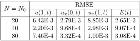
and (3.13), and the RMSE results are shown in Table 1. From this table it can be concluded that the BEM numerical solution is convergent to the corresponding exact values

u(1, t) =et, ux(0, t) = 0, ux(1, t) = 2et, E(t) =et/3, t∈[0,1], (4.3)

as the number of boundary elements increases.

Table 1: The RMSE foru(1, t),ux(0, t),ux(1, t) andE(t) obtained using the BEM for the direct

problem withN =N0 ∈ {20,40,80}, for Example 1.

N =N0 _{u(1, t) u} RMSE

x(0, t) ux(1, t) E(t)

20 6.43E-3 2.79E-3 8.85E-3 2.65E-3

40 2.20E-3 9.68E-4 2.98E-3 9.07E-4

80 7.46E-4 3.32E-4 1.00E-3 3.08E-4

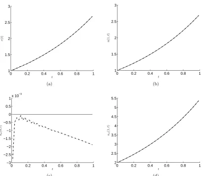
Next, we consider the inverse problem (1.1)–(1.3), (1.5) and (1.6) and we use the BEM with N = N0 = 40 for solving the resulting system of equations (3.14). Figure 1 displays the

analytical and numerical results of r(t), u(1, t), ux(0, t), and ux(1, t) and very good agreement

can be observed.

In practice, the contamination of measured data by unplanned error is unavoidable. Thus we add noise to the input energy dataE(t) in (1.6) in order to test the stability of the solution. The perturbed input data E

¯

ϵ _{is defined as}

E ¯

ϵ _{= E}

¯ +¯ϵ, (4.4)

whereϵ

¯=random(

′_Normal′_{,0, σ, N,1) is a set ofN variables generated randomly by the}

MAT-LAB command from a normal distribution with the zero mean and standard deviationσ given by

σ =p_× max

t∈[0,T]|E(t)|=

ep

3, (4.5)

where p is the percentage of noise. This perturbation means that the known right-hand side vector y

¯ is contaminated with noise, denoted as y¯

ϵ_{. Then, when noise is present, we have to}

solve the following system of linear equations instead of (3.14):

Xr ¯= y_¯

ϵ_{. (4.6)}

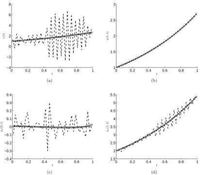
Figure 2 illustrates the analytical and numerical results for p= 1% noise in the input data (4.4) obtained by the straightforward inversion of (4.6), i.e. r

¯=X

−1_y

¯

ϵ_{. From this figure it can}

be seen that the numerical solutions for r(t), ux(0, t) and ux(1, t) shown by the dash-dot line

(_{− · −}) are unstable. However, the result for u(1, t) seems to remain stable.

To overcome this instability, we employ the second-order Tikhonov regularization method which gives

r ¯λ =

(

XtrX+λR₂trR2 )−1

Xtry ¯

0 0.2 0.4 0.6 0.8 1 1

1.5 2 2.5 3

t

r

(

t

)

(a)

0 0.2 0.4 0.6 0.8 1 1

1.5 2 2.5 3

t

u

(1

,

t

)

(b)

0 0.2 0.4 0.6 0.8 1 −3

−2.5 −2 −1.5 −1 −0.5 0 0.5

1x 10

−3

t

ux

(0

,

t

)

(c)

0 0.2 0.4 0.6 0.8 1 2

2.5 3 3.5 4 4.5 5 5.5

t

ux

(1

,

t

)

(d)

Figure 1: The analytical (—–) and numerical results (_{− · −}) of (a)r(t), (b)u(1, t), (c) ux(0, t),

and (d)ux(1, t) for exact data, for Example 1.

whereλ >0 is a regularization parameter to be prescribed andR2 is a second-order differential

regularization matrix, given by [15, 29],

Rtr₂ R2 =

1 (T /N)4



    

1 ₋2 1 0 0 . . .

−2 5 ₋4 1 0 . . .

1 ₋4 6 ₋4 1 0 . .

0 1 ₋4 6 ₋4 1 0 .

. . . .



    

. (4.8)

As it happened previously with some of our investigations [13, 14], we report that the second-order Tikhonov regularization has produced more accurate results than the zeroth- or first-second-order regularization and therefore, only the numerical results obtained using the former regularization are illustrated in this section.

A popular method for choosing the regularization parameter is the generalised cross-validation (GCV) criterion, which is based on minimising the following GCV function, [32]:

GCV(λ) = ∥X

(

Xtr_X+λRtr 2R2

)−1

Xtr_y

¯

ϵ_−y

¯

ϵ_∥2

[trace(I ₋X(Xtr_X+λRtr

2 R2)−1Xtr)]2

. (4.9)

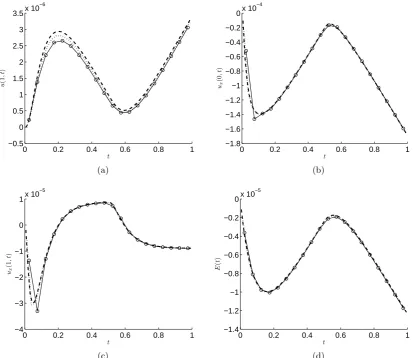
Then the numerical results obtained using (4.7) with this value ofλ, illustrated by circles (_{◦ ◦ ◦}) in Figure 2, show that accurate and stable numerical solutions are achieved.

0 0.2 0.4 0.6 0.8 1 −4

−2 0 2 4 6 8

t

r

(

t

)

(a)

0 0.2 0.4 0.6 0.8 1 1

1.5 2 2.5 3

t

u

(1

,

t

)

(b)

0 0.2 0.4 0.6 0.8 1 −0.4

−0.3 −0.2 −0.1 0 0.1 0.2 0.3 0.4

t

ux

(0

,

t

)

(c)

0 0.2 0.4 0.6 0.8 1 1.5

2 2.5 3 3.5 4 4.5 5 5.5

t

ux

(1

,

t

)

(d)

Figure 2: The analytical (—–) and numerical results of (a) r(t), (b) u(1, t), (c) ux(0, t), and

(d) ux(1, t) obtained using the straightforward inversion (− · −) with no regularization, and

the second-order Tikhonov regularization (_{◦ ◦ ◦}) with the regularization parameter λ=4.3E-6 suggested by the GCV method, forp= 1% noise, for Example 1.

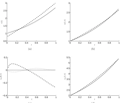
Next, we increase to p = 3% and 5% the percentage of noise with which the data (4.4) is contaminated. Figure 3 presents the analytical and numerical results obtained using the second-order Tikhonov regularization with the regularization parameter suggested by the GCV method, namelyλ=7.4E-6 for p= 3%, and λ=2.7E-5 for p= 5%. From this figure one can observe that stable and accurate results forr(t),u(1, t), ux(0, t) andux(1, t) withp= 3% noise are attained,

0 0.2 0.4 0.6 0.8 1 0.5

1 1.5 2 2.5 3

t

r

(

t

)

(a)

0 0.2 0.4 0.6 0.8 1 1

1.5 2 2.5 3

t

u

(1

,

t

)

(b)

0 0.2 0.4 0.6 0.8 1 −0.4

−0.2 0 0.2

t

ux

(0

,

t

)

(c)

0 0.2 0.4 0.6 0.8 1 2

2.5 3 3.5 4 4.5 5 5.5

t

ux

(1

,

t

)

(d)

Figure 3: The analytical (—–) and numerical results of (a) r(t), (b) u(1, t), (c) ux(0, t), and

(d) ux(1, t) obtained using the second-order Tikhonov regularization with the regularization

parameter suggested by the GCV method, forp= 3% (_{· · ·}) andp= 5% (_{− − −}), for Example 1.

Table 2: The regularization parametersλand the RMSE for r(t), u(1, t), ux(0, t) andux(1, t),

obtained using the BEM withN =N0 = 40 combined with the second-order Tikhonov

regular-ization forp_{∈ {}0,1,3,5_}% noise, for Example 1.

p λ RMSE

r(t) u(1, t) ux(0, t) ux(1, t)

0 (no noise) 0 4.16E-3 2.47E-4 1.20E-3 8.85E-4

1% 0 2.70 1.72E-2 1.12E-1 2.64E-1

1% 4.3E-6 1.73E-2 2.57E-3 8.92E-3 5.47E-3

3% 0 5.21 4.13E-2 3.51E-1 5.02E-1

3% 7.4E-6 3.32E-2 9.73E-3 1.97E-2 2.25E-2

5% 0 4.74 5.51E-2 4.64E-1 4.54E-1

5% 2.7E-5 1.95E-1 4.63E-2 1.29E-1 9.79E-2

4.2 Example 2

Φ4_n0[0,1]. Therefore, in this subsection we aim to construct an example for which the conditions of existence and uniqueness of solution of Theorem 1 are satisfied. We chooseT = 1, φ(x) = 0,

a=d= 1 and b= 0.

In the case a = d = 1, b = 0 the problem (1.8) has the eigenvalues µn = νn2, where νn

are the positive roots of the transcendental equation νsin(ν) = cos(ν). The corresponding eigenfunctions are yn(x) = sin(νnx). The first eigenvalue is given by ν0 = √µ0 = 0.860333.

Then choosing f(x, t) =x3(1₋x)4(β1x+β2) we can determine the constants β1 and β2 such

thatf _∈Φ4

0[0,1] (choosing n0 = 0 for simplicity), as required by the condition (A3) of Theorem

1. This imposes

0 =

∫ 1

0

f(x, t) sin(ν0x)dx= ∫ 1

0

x3(1₋x)4(β1x+β2) sin(ν0x)dx.

After some calculus, choosingβ2 =−1 it follows that β1 ≈2.011. With these values of β1 and

β2 we also satisfy that ∫₀1f(x, t)dx=−0.00037 is non-zero, as required by condition (A3). We

aim to retrieve a non-smooth source function given by

r(t) =

t₋1

2

, t_∈[0, t]. (4.10)

In this case, the analytical solution of the direct problem for the temperature u(x, t) is not available. Thus the energy E(t) is not available either. In such a situation, we simulate the data (1.6) numerically by solving first the direct problem (1.1)–(1.3) and (1.5) withr known and given by (4.10). The numerical solutions for u(1, t), ux(0, t), ux(1, t) and E(t) obtained using

the BEM with N = N0 ∈ {20,40,80} are shown in Figure 4. From this figure it can be seen

that convergent numerical solutions are obtained.

To investigate the inverse problem (1.1)–(1.3), (1.5) and (1.6), we use the numerical results for E(t) in Figure 4(d) obtained using the BEM with N = N0 = 40, as the input data (1.6).

In order to avoid committing an inverse crime we keep N = 40, but we use a different N0,

say N0 = 30, than 40 which was used in the direct problem simulation. Figure 5 shows the

numerical results obtained without regularization, i.e. λ = 0, for p = 0 (exact) and p = 1% (noisy) data. Remark that from Figure 4(d), the standard deviation in (4.5) for Example 2 is given byσ= 1.2_×10−5_{p. From Figure 5 it can be seen that, for exact data, the straightforward}

inversion of (3.14) produces very accurate results. However, when noise is introduced into the measured data (4.4), the numerical retrievals of especially r(t) and ux(1, t) become highly

oscillatory unstable.

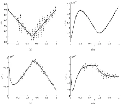
In order to retrieve the stability, as in Example 1, the second-order Tikhonov regularization with the GCV criterion are employed and the numerically obtained results are shown in Figure 6. The numerical results from the direct problem presented in Figures 4(a)–4(c) are used to compare in Figures 6(b)–6(d) the numerical results foru(1, t), ux(0, t), and ux(1, t), respectively, of the

inverse problem. Whereas the numerical solution for r(t) of the inverse problem is compared with the analytical solution (4.10) in Figure 6(a). From Figure 6 it can be seen that stable and accurate numerical solutions are obtained. For completeness, the RMSE errors (4.1) and the GCV values forλare displayed in Table 3.

0 0.2 0.4 0.6 0.8 1 −0.5

0 0.5 1 1.5 2 2.5 3 3.5x 10

−6

t

u

(1

,

t

)

(a)

0 0.2 0.4 0.6 0.8 1 −1.8

−1.6 −1.4 −1.2 −1 −0.8 −0.6 −0.4 −0.2

0x 10

−4

t

ux

(0

,

t

)

(b)

0 0.2 0.4 0.6 0.8 1 −4

−3 −2 −1 0 1x 10

−5

t

ux

(1

,

t

)

(c)

0 0.2 0.4 0.6 0.8 1 −1.4

−1.2 −1 −0.8 −0.6 −0.4 −0.2

0x 10

−5

t

E

(

t

)

(d)

Figure 4: The numerical results of (a)u(1, t), (b)ux(0, t), (c)ux(1, t), and (d)E(t) obtained by

solving the direct problem withN =N0 ∈ {20(◦ ◦ ◦), 40(· · ·), 80(− − −)}, for Example 2.

Finally, although not illustrated, it is reported that for both Examples 1 and 2 we have experienced with other values ofλclose to the optimal ones but there was not much significant difference obtained in comparison with the numerical results of Figures 2, 3 and 6. This con-firms that the GCV criterion performs well in choosing a suitable regularization parameter for obtaining a stable and accurate numerical solution.

5

Conclusions

The inverse problem of finding the time-dependent heat source together with the temperature in the heat equation, under a non-classical dynamic boundary condition and an integral over-determination condition has been investigated. Firstly, the existence, uniqueness, and continuous dependence upon the data of the classical solution of the inverse problem have been established. Next, a numerical method based on the BEM combined with the second-order Tikhonov regu-larization has been proposed together with the use of the GCV criterion for the selection of the regularization parameter. The retrieved numerical results were found to be accurate and stable on both smooth and non-smooth continuous examples.

0 0.2 0.4 0.6 0.8 1 −0.1

0 0.1 0.2 0.3 0.4 0.5 0.6

t

r

(

t

)

(a)

0 0.2 0.4 0.6 0.8 1 0

0.5 1 1.5 2 2.5 3 3.5x 10

−6

t

u

(1

,

t

)

(b)

0 0.2 0.4 0.6 0.8 1 −2

−1.5 −1 −0.5

0x 10

−4

t

ux

(0

,

t

)

(c)

0 0.2 0.4 0.6 0.8 1 −4

−3 −2 −1 0 1 2x 10

−5

t

ux

(1

,

t

)

(d)

Figure 5: The analytical solution (4.10) and the direct problem numerical solution from Figures 4(a)–4(c) (—–) and numerical results of (a)r(t), (b) u(1, t), (c)ux(0, t), and (d) ux(1, t), with

no regularization, for exact data (_{◦ ◦ ◦}) and noisy datap= 1% (_{− · −}), for Example 2.

only remark that unlike certain applications, e.g. some significant mismatch has been reported in [1, 23, 27] between experimental data of electromagnetic waves propagating in a non-attenuating medium and data produced by idealized computational simulations, in inverse heat conduction the mathematical models have been shown to perform much better in industrial applications with actual real measured data, [9].

Acknowledgements

A. Hazanee would like to acknowledge the financial support received from the Ministry of Science and Technology of Thailand, and Prince of Songkla University Thailand, for pursuing her PhD at the University of Leeds. The comments and suggestions made by the referees are gratefully acknowledged.

References

0 0.2 0.4 0.6 0.8 1 0

0.1 0.2 0.3 0.4 0.5 0.6

t

r

(

t

)

(a)

0 0.2 0.4 0.6 0.8 1 0

0.5 1 1.5 2 2.5 3 3.5x 10

−6

t

u

(1

,

t

)

(b)

0 0.2 0.4 0.6 0.8 1 −2

−1.5 −1 −0.5

0x 10

−4

t

ux

(0

,

t

)

(c)

0 0.2 0.4 0.6 0.8 1 −3

−2 −1 0 1

x 10−5

t

ux

(1

,

t

)

(d)

Figure 6: The analytical solution (4.10) and the direct problem numerical solutions from Figures 4(a)–4(c) (—–), and the numerical results of (a) r(t), (b) u(1, t), (c) ux(0, t), and (d) ux(1, t)

obtained using the second-order Tikhonov regularization with the regularization parameters suggested by GCV method, forp_{∈ {}1(_{◦ ◦ ◦}), 3(_{· · ·}), 5(_{− − −})_}% noise, for Example 2.

30_{, 025002 (24 pages).}

[2] Binding, P. A., Brown, P. J., and Seddeghi, K. (1993). Sturm-Liouville problems with eigenparameter dependent boundary conditions. Proceedings of the Edinburgh Mathematical Society,37_{, 57–72.}

[3] Bourgeois, L., Chaulet, N., and Haddar, H. (2011). Stable reconstruction of generalized impedance boundary conditions. Inverse Problems,27_{, 095002 (26 pages).}

[4] Bourgeois, L., Chaulet, N., and Haddar, H. (2012). On simultaneous identification of a scatterer and its generalized impedance boundary conditions. SIAM Journal on Scientific Computing,34_{, 1824–1848.}

[5] Bourgeois, L. and Haddar, H. (2010). Identification of generalized impedance boundary conditions in inverse scattering problems. Inverse Problems and Imaging,4_{, 19–38.}

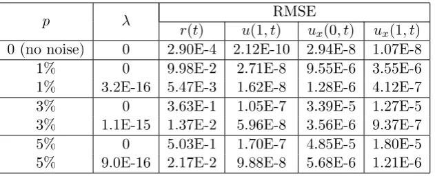
Table 3: The regularization parametersλand the RMSE for r(t), u(1, t), ux(0, t) andux(1, t),

obtained using the BEM with N = 40 and N0 = 30 combined with the second-order Tikhonov

regularization forp_{∈ {}0,1,3,5_}% noise, for Example 2.

p λ RMSE

r(t) u(1, t) ux(0, t) ux(1, t)

0 (no noise) 0 2.90E-4 2.12E-10 2.94E-8 1.07E-8

1% 0 9.98E-2 2.71E-8 9.55E-6 3.55E-6

1% 3.2E-16 5.47E-3 1.62E-8 1.28E-6 4.12E-7

3% 0 3.63E-1 1.05E-7 3.39E-5 1.27E-5

3% 1.1E-15 1.37E-2 5.96E-8 3.56E-6 9.37E-7

5% 0 5.03E-1 1.70E-7 4.85E-5 1.80E-5

5% 9.0E-16 2.17E-2 9.88E-8 5.68E-6 1.21E-6

[7] Cannon, J. R. (1984). The One-dimensional Heat Equation. Addison-Wesley Publishing Company, Menlo Park, California.

[8] Dragomir, S. S. (2002). Some Gronwall Type Inequalities and Applications. RGMIA Mono-graphs, Victoria University, Australia.

[9] Elden, L., Berntsson, F., and Reginska, T. (2000). Wavelet and Fourier methods for solving the sideways heat equation. SIAM Journal on Scientific Computing,21_{, 2187–2205.}

[10] Farcas, A. and Lesnic, D. (2006). The boundary element method for the determination of a heat source dependent on one variable. Journal of Engineering Mathematics,54_{, 375–388.}

[11] Fulton, C. T. (1977). Two-point boundary value problems with eigenvalue parameter con-tained in the boundary conditions. Proceedings of the Royal Society of Edinburgh: Section A Mathematics,77_{, 293–388.}

[12] Hasanov, A. and Pektas, B. (2013). Identification of an unknown time-dependent heat source term from overspecified Dirichlet boundary data by conjugate gradient method. Com-puters and Mathematics with Applications,65_{, 42–57.}

[13] Hazanee, A., Ismailov, M. I., Lesnic, D., and Kerimov, N. B. (2013). An inverse time-dependent source problem for the heat equation. Applied Numerical Mathematics,69_{, 13–33.}

[14] Hazanee, A. and Lesnic, D. (2013). Determination of a time-dependent heat source from nonlocal boundary conditions. Engineering Analysis with Boundary Elements,37_{, 936–956.}

[15] Hazanee, A. and Lesnic, D. (2014). Determination of a time-dependent coefficient in the bioheat equation. International Journal of Mechanical Sciences,88_{, 259–266.}

[16] Ionkin, N. I. (1977). Solution of a boundary-value problem in heat conduction with a non-classical boundary condition. Differential Equations,13_{, 294–304.}

[17] Ismailov, M. I., Kanca, F., and Lesnic, D. (2011). Determination of a time-dependent heat source under nonlocal boundary and integral overdetermination conditions. Applied Mathematics and Computation,218_{, 4138–4146.}

[18] Kapustin, N. Y. and Moiseev, E. I. (1997). Spectral problems with the spectral parameter in the boundary condition. Differential Equations,33_{, 115–119.}

[19] Kerimov, N. B. and Allakhverdiev, T. I. (1993a). On a certain boundary value problem I.

[20] Kerimov, N. B. and Allakhverdiev, T. I. (1993b). On a certain boundary value problem II.

Differential Equations,29_{, 952–960.}

[21] Kerimov, N. B. and Ismailov, M. I. (2013). Direct and inverse problems for the heat equation with a dynamic type boundary condition. IMA Journal of Applied Mathematics, submitted.

[22] Kerimov, N. B. and Mirzoev, V. S. (2003). On the basis properties of one spectral problem with a spectral parameter in a boundary condition. Siberian Mathematical Journal,44_{, 813–}

816.

[23] Kuzhuget, A. V., Beilina, L., Klibanov, M., Sullivan, A., Nguyen, L., and Fiddy, M. A. (2000). Blind experimental data collected in the field and an approximately globally conver-gent inverse algorithm. Inverse Problems,28_{, 095007 (33 pages).}

[24] Langer, R. E. (1932). A problem in diffusion or in the flow of heat for a solid in contact with a fluid. Tohoku Mathematical Journal,35_{, 360–375.}

[25] Lesnic, D., Elliott, L., Ingham, D. B., Knipe, R. J., and Clennell, B. (1996). The identi-fication of hydraulic conductivities of composite rocks. In Jones, G., Fisher, Q., and Knipe, R. J., editors, Faulting, Fault Sealing and Fluid Flow in Hydrocarbon Reservoirs: Abstracts, pages 113–114.

[26] Slodicka, M. (2014). A parabolic inverse source problem with a dynamic boundary condi-tion. Applied Mathematics and Computation, submitted.

[27] Thanh, N. T., Beilina, L., Klibanov, M., and Fiddy, M. A. (2014). Reconstruction of the refractive index from experimental backscattering data using a globally convergent inverse method. SIAM Journal on Scientific Computing,36_{, B273–B293.}

[28] Tichmarsh, E. C. (1962). Eigenfunction Expansions Associated with Second Order Differ-ential Equations I. Oxford University Press, Oxford.

[29] Twomey, S. (1963). On the numerical solution of Fredholm integral equations of the first kind by the inversion of the linear system produced by quadrature. Journal of the Association for Computing Machinery,10_{, 97–101.}

[30] Walter, J. (1973). Regular eigenvalue problems with eigenvalue parameter in the boundary conditions. Mathematische Zeitschrift,133_{, 301–312.}

[31] Xiong, X., Yan, Y., and Wang, J. (2011). A direct numerical method for solving inverse heat source problems. Journal of Physics: Conference Series,290_{, 012017 (10 pages).}

[32] Yan, L., Fu, C. L., and Yang, F. L. (2008). The method of fundamental solutions for the inverse heat source problem. Engineering Analysis with Boundary Elements,32_{, 216–222.}

[33] Yang, L., Dehghan, M., Yua, J. N., and Luoa, G. W. (2011). Inverse problem of time-dependent heat sources numerical reconstruction.Mathematics and Computers in Simulation,