White Rose Research Online URL for this paper:
http://eprints.whiterose.ac.uk/90730/
Version: Accepted Version
Article:
Salomon, S., Avigad, G., Purshouse, R.C. et al. (1 more author) (2015) Gearbox design for
uncertain load requirements using active robust optimization. Engineering Optimization.
ISSN 0305-215X
https://doi.org/10.1080/0305215X.2015.1031659
Reuse
Unless indicated otherwise, fulltext items are protected by copyright with all rights reserved. The copyright exception in section 29 of the Copyright, Designs and Patents Act 1988 allows the making of a single copy solely for the purpose of non-commercial research or private study within the limits of fair dealing. The publisher or other rights-holder may allow further reproduction and re-use of this version - refer to the White Rose Research Online record for this item. Where records identify the publisher as the copyright holder, users can verify any specific terms of use on the publisher’s website.
Takedown
If you consider content in White Rose Research Online to be in breach of UK law, please notify us by
To appear inEngineering Optimization Vol. 00, No. 00, Month 20XX, 1–20
Gearbox Design for Uncertain Load Requirements Using Active
Robust Optimization
Shaul Salomon†∗, Gideon Avigad‡, Robin C. Purshouse†, and Peter J. Fleming† †Department of Automatic Control and Systems Engineering, University of Sheffield, Sheffield, UK
‡Department of Mechanical Engineering,ORT Braude College of Engineering, Karmiel, IL
(Received 00 Month 20XX; final version received 00 Month 20XX)
Design and optimization of gear transmissions have been intensively studied, but surprisingly the robustness of the resulting optimal design to uncertain loads has never been considered. Active Robust (AR) optimization is a methodology to design products that attain robustness to uncertain or changing environmental conditions through adaptation. In this study the AR methodology is utilized to optimize the number of transmissions, as well as their gearing ratios, for an uncertain load demand. The problem is formulated as a bi-objective optimization problem where the objectives are to satisfy the load demand in the most energy efficient manner and to minimize production cost. The results show that this approach can find a set of robust designs, revealing a trade-off between energy efficiency and production cost. This can serve as a useful decision-making tool for the gearbox design process, as well as for other applications.
Keywords:Gearbox design; adaptive design; multi-objective optimization; robust optimization; active robustness.
1. Introduction
One of today’s engineers greatest challenge is the development of energy efficient products to cope with limited resources. In systems that include a gearbox, careful design of this component can enhance the efficiency of the system. A gearbox is an assembly of gears with different ratios that provides speed and torque conversions from a motor to another device. With the use of a gearbox, a single motor can meet a span of load demands, which are combinations of required speed and torque. There is a unique gearing ratio for every given motor that will result in the least energy consumption for a specific load demand. Usually a geared system operates under a range of possible loads. If optimality with respect to energy consumption is targeted, the gearbox should include an infinite number of gears in order to accommodate all loads within this range. Naturally it is not possible to produce such a gearbox, and anyway, a gearbox with too many gears has more drawbacks than advantages (e.g. dimensions, weight, costs). Therefore gearboxes used in real applications are made of a finite number of gears (typically up to six in the auto industry), where each gear covers a different range of the load demands (e.g. high reduction for high torque and low speed, and vice versa). The gearbox’s gearing ratios should allow for the satisfaction of each possible load by one of the gears in a reasonably efficient manner. Therefore, the choice of the gears determine the overall performance of
the gearbox. This choice can be supported by an optimization procedure for minimum energy consumption.
Some previous studies on gearbox optimization can be found in the literature.Guzzella and Amstutz (1999) presented a computer aided engineering tool for modelling and op-timization of a hybrid vehicle. They showed an example of optimizing the transmission ratios for minimum fuel consumption. The model is deterministic, and the ratios are opti-mized for a single, arbitrarily chosen, load cycle.Roos, Johansson, and Wikander (2006) suggested an optimization procedure for selecting a motor and gearhead for mechatronic applications aiming at either peak power, motor torque or energy efficiency. This ap-proach is suitable for a single gear system and not for a gearbox with several gears. The choice of the gearhead was conducted according to the worst case of the expected load scenarios. Swantner and Campbell (2012) developed a framework for gearbox optimiza-tion that searches among different types of gears (helical, conic, worm, etc.), topologies, materials and sizing parameters. The gearbox was optimized for minimum dimensions, considering a set of functional constraints. Other problem setting of single objective gearbox optimization include minimum variation from a given set of transmission ratios (Mogalapalli, Magrab, and Tsai 1992), minimum volume or weight (Yokota, Taguchi, and Gen 1998;Savsani, Rao, and Vakharia 2010), minimum vibration (Inoue, Townsend, and Coy 1992) or minimum center distance between input and output shafts (Li, Symmons, and Cockerham 1996).
Some multi-objective gearbox optimization studies can also be found in the litera-ture. Osyczka (1978) formulated a problem to minimize simultaneously four objective functions: volume of elements, peripheral velocity between gears, width of gearbox, and center distance. Wang (1994) considered center distance, weight, tooth deflection, and gear life as objective functions.Thompson, Gupta, and Shukla(2000) optimized for min-imum volume and surface fatigue life. Kurapati and Azarm (2000) optimized a gearbox for minimum volume and minimum stress in the output shaft. Deb, Pratap, and Moitra (2000) designed a compound gear train to achieve a specific gear ratio. The objectives of the gear train design were minimum error between the obtained gear ratio and the required gear ratio and maximum size of any of the gears. Deb and Jain (2003) have optimized an 18-speed, 5-shafts gearbox for two, three and four objectives. Among the objectives were power, volume, center distance and variation from desired output speed. The same optimization problem was used by Deb (2003) to demonstrate how design principles can be extracted by investigating the relations between design variables of the Pareto optimal solutions in the design space. Li et al.(2008) optimized a two-stage gear reducer for minimum dimensions, minimum contact stress and minimum transmission precision errors.
The optimization involved within all studies above was conducted for given reduction ratios, or at least for a given speed-torque scenario or cycle. However, most applications that include a gearbox (such as vehicles) are subjected to a large span of uncertain load requirements, as a result of a variety of possible environmental conditions. The stochas-tic nature of the required torque and speed must be considered during the design phase. In order to optimize a gearbox for uncertain load requirements, a robust optimization (RO) procedure should be considered. A robust solution is a solution that can maintain good performance over the various scenarios associated with the involved uncertainties. Robustness is usually attained at the price of not achieving peak performance in any spe-cific scenario, and the success of a solution to a robust optimization problem is measured according to a certain criterion such as its mean or worst performance (Paenke, Branke, and Jin 2006). In this study, a gearbox is optimized for minimum energy consumption where the load demand is uncertain. A robust set of transmission ratios is searched for to maximize the system’s efficiency considering the uncertain load domain.
properties that reduce the possible negative influences caused by uncontrolled parame-ters’ variations (e.g. thick insulation may reduce fluctuations of an oven internal temper-ature, caused by changes in the ambient temperature). When this is the case, robustness is passively attained without any action required from the user. A gearbox, however, can-not be optimized for robustness with this approach, since its performance does can-not solely depend on its preliminary design. The performance is also influenced by the manner in which the gearbox is being operated. A gearbox with a good selection of gearing ratios for a span of load scenarios can be very inefficient if it is not being used properly. For best performance, the proper gear in the set has to be selected for each realization of the uncertain load demand. When cruising on the highway, the best efficiency is achieved with the highest gear (say sixth). A driver that uses the fifth gear for this scenario does not operate the gearbox in an optimal manner. Hence, robustness to the uncertain load demand is actively attained by selecting the proper gear for each load scenario. The selection of the optimal gear for each scenario can be made either manually by a skilled user, or with the use of a controller in the case of an automatic transmission.
Theactive robustnessmethodology (AR), recently introduced bySalomon et al.(2014),
provides the required tools to conduct a robust optimization for a gearbox. AR aims at products that attain robustness to a changing or uncertain environment through adap-tation. Such products are termed as adaptive products. The AR methodology assumes that an adaptive product possess some properties that can be modified by its user. These properties allow the product to adapt to environmental changes in order to enhance op-timality. The adaptability of a geared system is provided by the user’s ability to change the gear ratios by altering the engaging wheels. This adaptability is taken into account at the evaluation of a candidate solution; it is evaluated according to its best possible performance for each scenario of the uncertain parameters. For the example above, it is assumed that the driver uses the sixth gear while cruising on the highway and sec-ond gear when carrying a heavy load up the hill. Since enhanced adaptability usually comes with a price (e.g., a gearbox with more gears would be more expensive), the objec-tives of anActive Robust Optimization Problem(AROP) are the solution’s best possible performance, evaluated at different scenarios of the uncertainties involved, and its cost.
The problem formulated in this paper is the optimization of a gearbox for a random variate of torque and speed requirements. Both the number of gears and their charac-teristics are optimized in order to minimize the overall energy consumption and gearbox cost. The solution to the problem is a set of gearboxes with a trade-off between energy efficiency and low cost. The AR optimization approach is demonstrated with a power system of a DC motor and a simple two stage reduction gearbox. The approach can be adopted to other geared systems such as vehicles, motorcycles, wind turbines, industrial and agricultural machinery.
The reminder of the paper is organised as follows: In Section2the required background
on Robust Optimization and Active Robust Optimization is provided. In Section 3 an
2. Background
2.1 Multi-Objective Optimization
Multi-objective optimization problems (MOPs) arise in many real-world applications, where multiple conflicting objectives should be simultaneously optimized. In the absence of prior subjective preference, the solution to such problems is a set of optimal “trade off” solutions rather than a single solution. This set is also called “Pareto optimal set” or “non-dominated set”. A non-dominated solution is a solution where none of the other solutions is better than it with respect to all of the objective functions.
Mathematically, a MOP can be defined as:
min
x∈Xζ(x,p) = [f1(x,p), . . . , fm(x,p)], (1)
wherexis annx-dimensional vector of decision variables in some feasible regionX ⊂Rnx
,
p is an np-dimensional vector of environmental parameters that are independent of the
design variables x and ζ is an m-dimensional performance vector.
The following define the Pareto optimal set, which is the solution to a MOP:
• A vectora= [a1, . . . , an] is said todominate another vectorb= [b1, . . . , bn] (denoted
asa≺b) if and only if ∀i∈1, . . . , n:ai ≤bi and ∃i∈1, . . . , n:ai < bi.
• A solutionx∈ X is said to bePareto optimalinX if and only if¬∃ˆx∈ X :ζ(ˆx,p)≺
ζ(x,p).
• The Pareto optimal set(PS) is the set of all Pareto optimal solutions, i.e.,
P S={x∈ X | ¬∃xˆ ∈ X :ζ(ˆx,p)≺ζ(x,p)}.
• The Pareto optimal front(PF) is the set of objective vectors corresponding to the
solutions in the PS, i.e., P F ={ζ(x,p)|x∈P S}.
2.2 Robust Optimization
Robust performance design tries to ensure that performance requirements are met and constraints are not violated due to system uncertainties and variations. The uncertainties may beepistemic, resulting from missing information about the system, oraleatory, where the system’s variables inherently change within a range of possible values. Fundamentally, robust optimization is concerned with minimizing the effect of such variations without eliminating the source of the uncertainty or variation (Phadke 1989).
The performance vectorζin Equation (1) might possess uncertain values due to several sources of uncertainties, which can be categorised according toBeyer and Sendhoff(2007) as follows:
(1) Changing environmental and operating conditions. In this case, the values of some
uncontrollable parametersp are uncertain. The reasons for uncertainty might be in-complete knowledge concerning these parameters, or expected changes in parameter values during system operation.
(2) Production tolerances and deterioration. These uncertainties occur when the actual
values of design variables differ from their nominal values. The deviation might occur during production (manufacturing tolerances) or during operation (deterioration). Here, thexvariables in Equation (1) are the source of uncertainty.
(3) Uncertainties in the system output. The actual value of the performance vector ζ
might differ from its measured or simulated value, due to measurement noise or model inaccuracies, respectively.
con-straint functions, which define optimality and feasibility, become uncertain too. To assess the uncertain functions, robustness and reliability are considered (Schu¨eller and Jensen 2008). Robustness can be seen as having good performance (i.e. objective function val-ues) regardless of the realisation of the uncertain conditions. Reliability is concerned with remaining feasible despite the uncertainties involved.
This study aims at a robust design for changing operating conditions. The related robust optimization problem can be formulated as:
min
x∈XF(x,P), (2)
wherexis annx-dimensional vector of decision variables in some feasible regionX ⊂Rnx, P is an np-dimensional vector random variate, of uncertain environmental parameters
that are independent of the design variablesx, andF(x,P) is a distribution of objective function values that correspond to the variate of the uncertain parameters P.
In a robust optimization scheme, the random objective function is evaluated according to a robustness criterion, denoted by an indicator φ[F]. Three classes of criteria are presented in the following.
Worst-case optimization, also known as robust optimization in the operational research literature (Bertsimas, Brown, and Caramanis 2011) or minmax optimization (Alicino and Vasile 2014), considers the worst performance of a candidate solution over the entire range of uncertainties. The worst-case indicator for a minimzation problem can be written as:
φw[F(x,P)] := max
p∈PF(x,P). (3)
The robust optimisation problem in Equation (2) then reads:
min
x∈Xmaxp∈PF(x,P). (4)
To address the tendency of this approach to produce over-conservative solutions, Jiang, Wang, and Guan(2012) suggested a method for controlling the conservatism of the search by reducing the size of the uncertainty interval with a tuneable parameter. Branke and Rosenbusch(2008) suggested an evolutionary algorithm for worst-case optimization that simultaneously searches for the robust solution and the worst-case scenario by co-evolving the population of scenarios alongside the candidate solutions.
Aggregation methods use an integral measure that amalgamates the possible values of the uncertain objective function. The most common aggregated indicators are the expected value of the objective function or its variance – see the review by Beyer and Sendhoff (2007). When the distribution of the uncertain parameters can be described by the probability density function ρ(p), the mean value criterion can be computed by:
φm[F(x,P)] :=
Z
p∈P
f(x,p)ρ(p)dp, (5)
then becomes:
φmF x,P:= 1
k
k
X
1=1
f(x,pi), (6)
wherepi is theithsample inP.Kang, Lee, and Lee(2012) have considered the expected
value with a partial mean of costs to solve a process design robust optimization problem. Kumar et al. (2008) have used Bayesian Monte-Carlo sampling to construct a sampled representation for the performance of candidate compressor blades. They considered both the mean value and the variance as a multi-objective optimization problem, and used a multi-objective evolutionary algorithm to search for robust solutions. An alternative formulation is to aggregate the mean and variance into a single objective function (e.g. Lee and Park 2001).
Beyer and Sendhoff (2007) suggested a criterion that uses the probability distribution of the objective function directly as a robustness measure. This is done by setting a performance goal, and maximising the probability for achieving this goal, i.e. for the function value to be better than a desired threshold. Considering a performance threshold
q, a threshold probability indicator can be defined as:
φtp[F(x,p)] := Pr F(x,p)< q. (7)
Reliability-based design aims at minimizing the risk of failure during the product ex-pected lifecycle (Schu¨eller and Jensen 2008). In the context of design optimization, it can be seen as minimizing the risk of violating the problem’s constraints. The criteria mentioned above for robustness can also be used to assess reliability by applying them to the constraint functions. A conservative worst-case approach was used by several au-thors (e.g. Avigad and Coello 2010; Albert et al. 2011). The “six-sigma” methodology (see Brady and Allen 2006) suggests a goal of 3.4 defects per million products, which sets a threshold probability for reliability.
2.3 Active Robustness Optimization Methodology
The AR methodology (Salomon et al. 2014), is a special case of robust optimization, where the product has some adjustable properties that can be modified by the user after the optimized design has been realized. These adjustable variables allow the product to adapt to variations in the uncontrolled parameters, so it can actively suppress their nega-tive effect. The methodology makes a distinction between three types of variables: design variables, denoted asx, adjustable variables, denoted asy and uncontrollable stochastic parameters P. A single realized vector of uncertain parameters from the random variate
P is denoted asp.
In a conventional robust optimization problem, each realization p is associated with a corresponding objective function value f(x,p), and a solution x is associated with a distribution of objective function values that correspond to the variate of the uncertain parameters P. This distribution is denoted as F(x,P). In active robust optimization, for every realization of the uncertain environment, the performance also depends on the value of the adjustable variables y, i.e., f ≡ f(x,y,p). Since the adjustable variables’ values can be selected after p is realized, the solution can improve its performance by adapting its adjustable variables to the new conditions. In order to evaluate the solution’s performance according to the robust optimization methodology, it is conceivable that the
selected. This can be expressed as the optimal configurationy⋆:
y⋆ = argmin
y∈Y(x)
f(x,y,p), (8)
whereY(x) is the solution’s domain of adjustable variables, also termed as the solution’s adaptability.
Considering the entire environmental uncertainty, a one-to-one mapping between the scenarios in Pand the optimal configurations in Y(x) can be defined as:
Y⋆ = argmin
y∈Y(x)
F(x,y,P). (9)
Assuming a solution will always adapt to its optimal configuration, its performance can be described by the following variate:
F(x,P)≡F(x,Y⋆,P). (10)
An Active Robust Opimization Problem(AROP) comes to minimize the performance
indicator φ for the variate F(x,Y⋆,P). It is denoted as φ(x,Y⋆,P). Since enhanced performance usually increases the costs of the product, the aim of an AROP is to find solutions that are both robust and inexpensive. Therefore the AROP is a multi-objective problem that simultaneously optimizes the performance indicator φ and the solution’s cost.
The cost function for the gearbox that is used in this study only depends on the gearbox’s preliminary design, i.e., the number of gears and their specifications. Therefore it is not affected by the uncertain load demand and has a deterministic value. The general definition of an AROP considers a stochastic distribution of the cost function, but in this case it is denoted as c(x).
Following the above, the Active Robust Opimization Problem is formulated:
min
x∈Xζ(x,P) = [φ(x,Y
⋆,P), c(x)], (11)
where Y⋆= argmin
y∈Y(x)
F(x,y,P). (12)
It is a multi-stage problem. In order to compute the objective function φ in Equa-tion (11), the problem in Equation (12) has to be solved for every solution x with the entire environment universe P. In a typical implementation the environmental uncer-tainty Pis sampled using Monte Carlo methods. This sample, P, leads to sample-based representations ofY⋆ andF – denotedY⋆andFrespectively. This leads to an estimated
performance vector ζ.
3. Motor and Gear System
The problem at hand is the optimization of a gearbox for a span of torque-speed scenarios. A DC motor of type Maxon A-max 32 is to convey a torqueτLat speedωL. In order to do
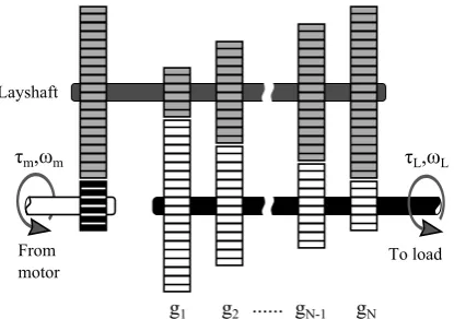
so, it is coupled with a gearbox as shown in Figure 1. The motor’s output shaft (white) rotates at speed ωm and transmits a torque τm. It is firmly connected to a cogwheel
(black) that is constantly coupled to the layshaft. The layshaft consists of a shaft and
Figure 1. A gearbox with N gears. All gears are rotating while at any given moment the power is transmitted through one of them.
are constantly coupled to the layshaft and rotate at different speeds, depending on the gearing ratio. A collar (not shown in the figure) is connected, through splines, to the load shaft and spins with it. It can slide along the shaft to engage either of the gears, by fitting teeth called “dog teeth” into holes on the sides of the gears. In that manner the power is transferred to the load through a certain gear, with the desired reduction ratio. The aim of this study is to optimize the gearbox to achieve good performance over a variety of possible load scenarios. Several objectives might be considered: monetary costs, energy efficiency for different loads and the transient behaviour of the gearbox (e.g. energy consumption during speed transitions and time required to change the system’s speed). A problem formulation that considers all of the aforementioned objectives is very complex and challenging. However, in order to demonstrate the features and concerns of the active robustness approach, at this stage it is sufficient to focus on a more restricted formulation of the gearbox optimization problem. Therefore, only the steady-state behaviour of the gearbox is addressed in this study.
The number of gears in the gearbox, N, and the number of teeth in each ith gear,z
i,
are to be optimized. The objectives considered are minimum energy consumption and minimum manufacturing cost of the gearbox. The system is evaluated at steady-state, i.e., operating at the torque-speed scenarios. The power required for each scenario is considered, while the objective is to find the set of gears that will require the minimum average invested power over all scenarios. For every scenario, the gearbox is evaluated by the the smallest possible value of input power. This value is achieved by transmitting the power through the most suitable gear in the box.
3.1 Model Formulation
In this section, the model for the motor and gearbox system is presented according to Krishnan (2001), and the required performance measures are derived.
The motor armature current can be described by applying Kirchoff’s voltage law over the armature circuit:
V =LI˙+rI+kvωm, (13)
whereV is the input voltage,L is the coil inductance,I is the armature current,ris the armature resistance and kv is the velocity constant. The ordinary differential equation
[image:9.595.195.403.47.193.2]output shaft is:
Jmω˙m =ktI−bmωm−τm, (14)
where Jm is the rotor’s inertia,kt is the torque constant andbm is the motor’s damping
coefficient associated with the mechanical rotation. Since this study only deals with the gearbox’s performance at steady-state, the derivatives of I and ωm are considered as
zero.
There are two speed reductions between the motor and the load. The first is from the motor shaft to the layshaft. This reduction ratio, denoted as n1, is zl/zm, where zm is
the number of teeth in the motor shaft cogwheel and zl is the number of teeth in the
layshaft cogwheel. The second reduction, denoted as n2, is from the layshaft to the load shaft. Each gear on the load shaft rotates at a different speed according to its gearing ration2,i=zg,i/zl,i, wherezg,iis the number of teeth of theithgear’s load shaft cogwheel
and zl,i is the number of teeth of its matching layshaft wheel.n2depends on the selected gear, and it can be one of the values {n2,1, . . . , n2,N}. The total reduction ratio from the
motor to the load is n = n1 ∗n2, and the load speed ω =ωm/n. The motor and load
shafts are coaxial, and the modules for all cogwheels are identical. Therefore, the total number of teeth Ntfor each gearing couple is identical:
Nt=zl+zm =zg,i+zl,i , ∀i∈1, . . . , N. (15)
At steady-state, Equation (14) can be reflected to the load shaft as follows:
0 =nktI− bg+n2bm
ω−τ, (16)
where τ is the load’s torque and bg is the gear’s damping coefficient with respect to the
load’s speed.
If ω from Equation (16) is known, the armature current can be derived:
I = bg+n 2b
m
ω+τ nkt
. (17)
Once the current is known, and after neglecting ˙I, the required voltage can be derived from Equation (13):
V =rI+nkvω. (18)
The invested electrical power is:
s=V I. (19)
It is conceivable that manufacturing costs depend on the number of wheels in the gearbox, their size, and overheads. A function of this type is suggested for this generic problem to demonstrate how the various costs can be quantified:
c=αNβ+γ
N
X
i=1
zl,i2 +z2g,i
+δ, (20)
The second term relates to the cogwheels material costs, which are proportional to the square of the number of teeth in each wheel. The third represents the overheads. In practice, other cost functions could be used.
4. Problem Definition
The gearbox optimization problem, formulated as an AROP, is the search for the number of gearsN and the number of teeth in each gearzg,i that minimize the production costc
and the power input s. According to the AR methodology, introduced in Section2, the variables are sorted into three vectors:
• xis a vector with the variables that define the gearbox, namely the number of gears and their teeth number. These variables can be selected before the gearbox is produced, but cannot be altered by the user during its life cycle. The variables in x are the problem’s design variables.
• yis a vector with the adjustable variables. It includes the variables that can be adjusted by the gearbox’s user: the selected gear i and the supplied voltage V. The decisions how to adjust these variables are made according to the load’s demand, and can be supported by an optimization procedure. For example, a high reduction ratio will be chosen for low speed, and a low ratio for high speeds, while the voltage is adjusted to maintain the desired velocity for the given torque.
• p is a vector with all the environmental parameters that affect performance and are independent of the design variables. Some of the parameters in this problem are con-sidered as deterministic, but some possess uncertain values. The uncertainty forω and
τ is aleatory, since they inherently vary within a range of possible load scenarios. The random variates of ω and τ are denoted as Ω and T, respectively. Some values of the motor parameters are given tolerances by the supplier. The terminal resistance r has a tolerance of 5% and the motor resistance bm has a tolerance of 10%. Additionally,
the gearbox dampingbg can be only estimated, and therefore it is treated as an
epis-temic uncertainty. The random variates ofr,bm andbg are denoted asR,Bm andBg,
respectively. The resulting variate ofp is denoted asP.
A certain load scenario might have more than one feasible y configuration. When the gearbox (represented byx) is evaluated for each scenario, the optimal configuration (the one that requires the least input power) is considered. This configuration is denoted asy⋆, and it consists of the optimal transmission iand input voltageV for the given scenario. The variate of optimal configurations that correspond to the variate Pis termed as Y⋆.
Since the input power varies according to the uncertain parameters (this can be denoted as S(x,Y⋆,P)), a robust optimization criterion is used in order to assess its value. The
mean value is a reasonable candidate for this purpose, as it captures the efficiency of the gearbox when it operates over the entire range of expected load scenarios. It is denoted as π(x,Y⋆,P).
min
x∈Xζ(x,P) ={π(x,Y
⋆,P), c(x)},
Y⋆ = argmin
y∈Y(x)
S(y,P),
subject to : I ≤Inom,
zg,i+zl,i=Nt , ∀i= 1, . . . , N,
where : x= [N, zg,1, . . . , zg,i, . . . , zg,N],
y= [i, V],
P= [Ω,T, R, Bm, Bg, kv, kt, Inom, n1, Nt,
α, β, γ, δ].
(21)
The constraints are evaluated according to Equations (17) and (18), and the objectives according to Equations (19) and (20).Inom, the nominal current, is the highest continuous
current that does not damage the motor. It is significantly smaller than the motor’s stall current.
By operating with maximum input power (i.e. with maximum voltage and current), for each velocityω there is a single transmission ratio nthat would allow the maximum torque, denoted asτmax(ω). This torque can be derived from Equations (16) and (18) by
replacing I with Inom and V withVmax.
τmax(ω) = max
n∈Y nktInom− bg+n
2b
m
ω,
subject to : rInom+nkvω=Vmax,
(22)
where Y ⊂R is the range of possible reduction ratios for this problem. Since a gearbox in the above AROP consists of a finite number of gears, it cannot operate at τmax for most of the velocities. In order to obtain feasible solutions with five gears or less, the domain of possible scenarios in this example is assumed to be in the range of 0≤τ(ω)≤
0.55τmax(ω). The effects of this assumption on the obtained solutions’ robustness are further discussed in Section 5.2.
Some information on the probability of load scenarios is usually known in a typical gearbox design (e.g. drive cycle information in vehicle design). In this generic example this kind of information is not available, and therefore a uniform distribution is assumed. The other uncertainties are treated in a similar manner: A uniform distribution is assumed for
R and Bm, since the tolerance information provided by the manufacturer only specifies
the boundaries for the actual property values, but does not specify their distribution. The epistemic uncertainty regardingbg also results in a uniform distribution ofBg within
an estimated interval.
Monte-Carlo sampling is used to represent the uncertain parameter domain P. A set
P of size k, is constructed by a random sampling of P with an even probability. In this example, Pconsists of k = 1,000 scenarios. The choice of sample size is further investigated in Section 5.2. Figure 2 depicts the domain of load scenarios Ω and T, together with their samples in Pand the curveτmax(ω).
ω[rad sec]
0 50 100 150 200 250 300
τL
[
mN
m
]
0 50 100 150 200 250 300 350 400 450
torque-speed domain sampled scenario
τ
max(ω)
Figure 2. The possible domain of torque-speed scenarios, and a representative set randomly sampled with an even probability.
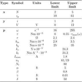
Table 1. Variables and parameters for the AROP in (21)
Type Symbol Units Lower Upper
limit limit
x N 2 5
zg 19 61
y i 1 N
V V 0 12
p ω s−1 16 295
τ Nm·10−3 0 0.55·τ
max(ω)
r Ω 2.1 2.4
bm Nm·s·10−6 2.8 3.5
bg Nm·s·10−6 25 35
kv V·s·10−3 24.3
kt Nm·A−1·10−3 24.3
Inom A 1.8
n1 61/19
Nt 80
α $ 5
β 0.8
γ $ 0.01
δ $ 50
5. Simulation Results
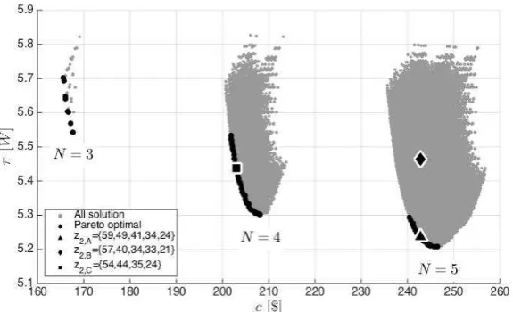
[image:13.595.166.424.61.253.2] [image:13.595.155.440.304.587.2]Figure 3. The objectives values of all feasible solutions to the problem in Equation (21) and Pareto front.
A feasible solution is a gearbox that has at least one gear that does not violate the constraints for each of the scenarios (i.e., I ≤ Inom and V ≤ Vmax). Figure 3 depicts
the objective space of the AROP. There are 194,861 feasible solutions (marked with gray dots), and the 103 non-dominated solutions are marked with black dots. It is noticed that the solutions are grouped into three clusters with a different price range for each number of gears. The three clusters correspond to N ∈ {3,4,5}, where fewer gears are related with a lower cost. None of the solutions with N = 2 is feasible.
5.1 A Comparison Between an Optimal Solution and a Non-Optimal
Solution
For a better understanding of the results obtained by the AR approach, two candi-date solutions are examined: one that belongs to the Pareto optimal front, and another that does not. Consider a scenario where lowest energy consumption is desired for a given budget limitation. For the sake of this example, a budget limit of $243 per unit is arbitrarily chosen. The gearbox with the best performance for that cost is marked in Fig-ure 3 as Solution A. This solution consists of five gears with z2,A = {59,49,41,34,24}
and corresponding transmission ratios nA = {9.02,5.07,3.38,2.37,1.38}. Another
so-lution with the same cost is marked in Figure 3 as Solution B. The gears of this solution are z2,B = {57,40,34,33,21}, and its corresponding transmission ratios are nB={7.96,3.21,2.37,2.25,1.14}.
Figure 4 depicts the set of optimal transmission ratio at every sampled scenario for both solutions. Each transmission is marked in the figure with a different marker. This set is in fact the set Y⋆from Equation (21), that correspond to the sampled set of load
scenarios P, in Figure 2. It is observed that the reduction ratios of Solution A almost form a geometrical series, where each consecutive ratio is divided by 1.6 approximately. The resulting Y⋆(x
A) is such that all gears are optimal for a similar number of load
scenarios. Solution B on the other hand has two gears with very similar ratios. It can be seen in Figure 4(b) that the third and the fourth gears are barely used. These gears do not contribute much to the gearbox’s efficiency, but significantly increase its cost. As can be seen in Figure 3, there are gearboxes with four gears that achieve the same or better efficiency as Solution B.
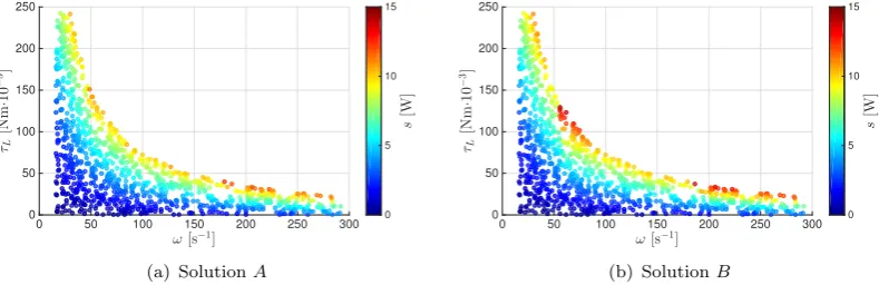
Figure5depicts the lowest power consumption for every sampled scenario,s x,Y⋆,P
ω[s−1]
0 50 100 150 200 250 300
τL [Nm · 10 − 3] 0 50 100 150 200
250 ratio @ gear
9.02 @ 1st 5.07 @ 2nd 3.38 @ 3rd 2.37 @ 4th 1.38 @ 5th
(a) SolutionA
ω[s−1]
0 50 100 150 200 250 300
τL [Nm · 10 − 3] 0 50 100 150 200
250 ratio @ gear
7.96 @ 1st 3.21 @ 2nd 2.37 @ 3rd 2.25 @ 4th 1.14 @ 5th
[image:15.595.104.491.55.186.2](b) SolutionB
Figure 4. Optimal transmission ratio for every sampled scenario. See online version for color display.
ω[s−1]
0 50 100 150 200 250 300
τL [Nm · 10 − 3] 0 50 100 150 200 250 s [W ] 0 5 10 15
(a) SolutionA
ω[s−1]
0 50 100 150 200 250 300
τL [Nm · 10 − 3] 0 50 100 150 200 250 s [W ] 0 5 10 15
(b) SolutionB
Figure 5. Lowest power consumption for every sampled scenario. See online version for color display.
in Figure 4). It can be seen that Solution A uses less energy at many load scenarios compared to Solution B. This is depicted by the darker shades of many of the scenarios in Figure 5(b). In order to assess the robustness, the mean input power π x,Y⋆,P
is used as the robustness criterion for this AROP. It is calculated by averaging the values of all points in Figure5. The results areπ xA,Y⋆,P
= 5.23W andπ xB,Y⋆,P
= 5.47W. Considering both solutions cost the same, this confirms Solution A’s superiority over Solution B. Given a budget limitation of $243, Solution A should be preferred by the decision maker.
5.2 Robustness of the Obtained Solutions
In this section the sensitivity of the AROP’s solution to several factors of the problem formulation is examined. Two aspects are considered with respect to different robustness metrics and parameter settings: i) the optimality of a specific solution, and ii) the differ-ence between two alternative solutions. For this purpose, three tests are performed. The first relates to the robustness of the solutions to epistemic uncertainty, namely the un-known range of load scenarios. The second test relates to the robustness of the solutions to a different robustness metric. The third test examines the sensitivity to the sampling size.
Sensitivity to Epistemic Uncertainty
[image:15.595.102.497.226.354.2]c[$]
120 140 160 180 200 220 240 260
π
[
W
]
3.5 4 4.5 5 5.5 6 6.5 7
N= 2
N= 3 N
= 4 N= 5
a = 70% a = 65% a = 60% a = 55% a = 50% a = 45% a = 40%
z2,A={59,49,41,34,24} z2,B={57,40,34,33,21} z2,C={54,44,35,24}
Figure 6. Pareto frontiers for different upper bounds of the uncertain load domaina·τmax(ω). See online version
for color display.
whereas for a= 70% the only feasible solutions are those with five gears. For percentiles larger than 70% there are no feasible solutions within the search domain.
To examine the effect of the choice of maximum torque percentile on the problem’s solution, the three solutions from Figure 3 are plotted for every percentile in Figure6. SolutionsAandC, who belong to the Pareto set fora= 55%, are also Pareto optimal for all other values ofasmaller than 65%. SolutionBremains dominated by both SolutionsA
andC. When very high performance is required (i.e. maximum torque percentiles of 65% or higher), both Solution Aand Solution C become infeasible.
It can be concluded that the mean value, as a robustness metric, is not sensitive to the maximum torque percentile. On the other hand, the reliability of the solutions, i.e. their probability to remain feasible, is sensitive to the presence of extreme loading scenarios.
Sensitivity to Preferences
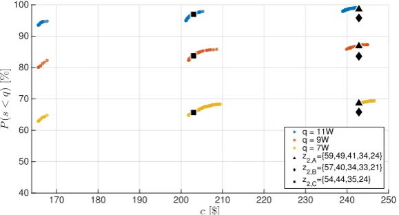
The threshold probability metric is used to examine the sensitivity of the solutions to different performance goals. It is defined for the above AROP as the probability for a solution to consume less energy than a predefined threshold:
φtp= Pr(S < q), (23)
where q is the performance goal. The aim is to maximize φtp.
Figure7depicts the results of the AROP described in Section4, whenφtpis considered as the robustness metric, and the goal performance is set to q = 5W. The same three solutions from Figure3are also shown here. SolutionA, whose mean power consumption is the best for its price, is not optimal any more when the probability of especially poor performance is considered. Solution A manages to satisfy the goal for 98.6% of the sampled scenarios, while another solution with the same price satisfies 99% of the scenarios. It is up to the decision maker to determine whether the difference between 98.6% and 99% is significant or not.
[image:16.595.154.440.58.229.2]Figure 7. The objectives values of all feasible solutions and Pareto front, for maximizing the threshold probability
φtp= Pr(S <11W).
c[$]
170 180 190 200 210 220 230 240 250
P
(
s
<
q
)
[%
]
40 50 60 70 80 90 100
q = 11W q = 9W q = 7W
z2,A={59,49,41,34,24}
z2,B={57,40,34,33,21}
[image:17.595.151.440.57.233.2]z2,C={54,44,35,24}
Figure 8. Pareto frontiers for different thresholdsq. See online version for color display.
Sensitivity to the Sampled Representation of Uncertainties
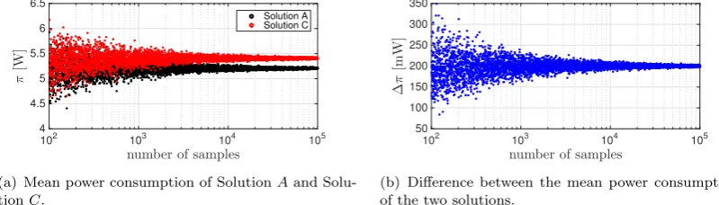
The random variates are represented in this study with a sampled set, using Monte-Carlo methods. The following experiment was conducted in order to verify that 1,000 samples are enough to provide a reliable evaluation of the solutions’ statistics: SolutionsA
and C were evaluated for their mean power consumption over 5,000 different sampled sets with sizes varying from k = 100 to k = 100,000. Figure 9(a) depicts the metric values of the solutions for every sample size. It is evident from the results that a large number of samples is required for the sampling error to converge. For both solution, the standard deviation is 15%, 6%, 2% and 0.5% of the mean value, for sample sizes of
k= 100,k= 1,000,k= 10,000, andk= 100,000, respectively. If an accurate estimate is required for the actual power consumption, a large sample size must be used (i.e. larger than k= 1,000 that was used in this study).
On the other hand, a comparison between two candidate solutions can be based on a much smaller sampled set. Although the values of π x,Y⋆,P
[image:17.595.152.442.292.448.2]number of samples
102 103 104 105
π
[W
]
4 4.5 5 5.5 6 6.5
Solution A Solution C
(a) Mean power consumption of SolutionAand Solu-tionC.
number of samples
102 103 104 105
∆
π
[m
W
]
50 100 150 200 250 300 350
(b) Difference between the mean power consumption of the two solutions.
Figure 9. Convergence of the mean power consumption of two solutions for different number of samples. See online version for color display.
solutions ∆π P
is defined:
∆π P
=π xC,Y⋆,P
−π xA,Y⋆,P
(24)
Figure 9(b) depicts the value of ∆π P
for every evaluated sampled set. It can be seen that ∆π converges to 200mW. For a sampling size of k = 100, the standard deviation of ∆π is 25mW, which is only 12% of the actual difference. This means that it can be argued with confidence that Solution A has better performance than SolutionC, based on a sample size of k= 100.
Based on the results from this experiment, it can be concluded that the solution to the AROP (i.e. the set of Pareto optimal solutions) is not sensitive to the sample size. The Pareto front shown in Figure 3 might be shifted along the π axes for different sampled representations of the uncertainties, but the same (or very similar) solutions would always be identified.
6. Conclusions
This study is the first of its kind to extend gearbox design optimization to consider the realities of uncertain load demand. It demonstrates how the stochastic nature of the uncertain load demand can be fully catered for during the optimization process using an Active Robustness approach. A set of optimal solutions with a trade-off between cost and efficiency was identified, and the advantages of a gearbox from this set over a non-optimal one were shown. The robustness of the obtained Pareto non-optimal solutions to several aspects of the problem formulation was verified.
The approach takes account of – and exploits – user influence on system performance, but presently assumes that the user is able to operate the gearbox in an optimal manner to achieve best performance. Of course, this assumption can only be fully validated if a skilled user or a well tuned controller activates the gearbox. This raises an important issue of how to train this user or controller to achieve best performance, which is identified as a priority for further research.
[image:18.595.94.494.59.173.2]solved off-line, before the product goes to manufacturing, supercomputing facilities are likely to be available, and a reasonable time-scale for solving the problem might be days or even a few weeks.
Adaptability is the solution’s ability to react to changes in its environment by adjust-ing itself to a configuration that improves its performance. In this study the gearbox’s adaptability was evaluated by only considering its performance at each of the sampled load scenarios, i.e., at steady-state. However, the Active Robustness methodology, pre-sented by Salomon et al. (2014), considers adaptability in a wider sense. In addition to its performance at steady-state, the solution’s transient behaviour during adaptation to environmental changes is also considered. For the problem presented in this paper, an environmental change is a change in demand from one load scenario to another. Al-though the optimal configurations can be found for both scenarios, the gearing ratios and input voltages applied while changing between these configurations may have a substan-tial impact on the solution’s performance. This notion was deliberately not considered in the current study in order to focus on basic aspects of the approach. An important extension to this work would be to examine the transient behaviour when evaluating a candidate solution. Additional objectives such as acceleration and energy consumption during adaptation can be examined by doing so. The Optimal Adaptation method ( Sa-lomon et al. 2013) can be used to search for adaptation trajectories that optimize these objectives.
The transient extension to the problem formulation requires extra considerations with respect to computational complexity. The two main reasons for this are: (a) A change between any two scenarios can be made by infinite possible gear sequences and voltage trajectories. This requires a search for the optimal trajectory in order to be consistent with the AR approach. This kind of search is usually computationally expensive. (b)
Each adaptation between two scenarios has to be examined. The number of possible adaptations betweenkscenarios arek(k−1). For the sampled set of 1,000 scenarios used in this study, there will be 999,000 adaptations to examine for each solution, implying a requirement to solve 999,000 optimization problems. As a part of future research, special attention should be given to model simplification and finding reliable ways to reduce the number of evaluated adaptations, e.g. by using efficient algorithms and sampling methods.
This initial study of gearbox optimization is based on a simple DC motor and gearbox. This is advantageous in focusing the presentation on the Active Robustness approach rather than, for example, constraint handling, and enables the objective functions to be calculated analytically. Additional applications for the AR methodology will be demon-strated in future publications, including more complex real-world geared systems.
Acknowledgement
References
Albert, Elvira, Samir Genaim, Miguel G´omez-Zamalloa, EinarBroch Johnsen, Rudolf Schlatte, and S.LizethTapia Tarifa. 2011. “Simulating Concurrent Behaviors with Worst-Case Cost Bounds.” In FM 2011: Formal Methods SE - 27, Vol. 6664 of Lecture Notes in Computer Science edited by Michael Butler and Wolfram Schulte. 353–368. Springer Berlin Heidelberg.
http://dx.doi.org/10.1007/978-3-642-21437-0_27.
Alicino, S, and M Vasile. 2014. “An evolutionary approach to the solution of multi-objective min-max problems in evidence-based robust optimization.” In Evolutionary Computation (CEC), 2014 IEEE Congress on,1179–1186.
Avigad, Gideon, and C. A. Coello. 2010. “Highly Reliable Optimal Solutions to Multi-Objective Problems and Their Evolution by Means of Worst-Case Analysis.”Engineering Optimization 42 (12): 1095–1117. http://www.tandfonline.com/doi/abs/10.1080/03052151003668151. Bertsimas, Dimitris, David B Brown, and Constantine Caramanis. 2011. “Theory and
Applica-tions of Robust Optimization.”SIAM Review 53 (3): 464–501.
Beyer, Hans Georg, and Bernhard Sendhoff. 2007. “Robust Optimization - A Comprehensive Survey.” Computer Methods in Applied Mechanics and Engineering 196 (33-34): 3190–3218.
http://linkinghub.elsevier.com/retrieve/pii/S0045782507001259.
Brady, James E, and Theodore T Allen. 2006. “Six Sigma Literature: A Review and Agenda for Future Research.”Quality and Reliability Engineering International 22 (3): 335–367. http: //dx.doi.org/10.1002/qre.769.
Branke, J¨urgen, and Johanna Rosenbusch. 2008. “New Approaches to Coevolutionary Worst-Case Optimization.” InParallel Problem Solving from Nature ? PPSN X SE - 15,Vol. 5199 of Lecture Notes in Computer Scienceedited by G¨unter Rudolph, Thomas Jansen, Simon Lucas, Carlo Poloni, and Nicola Beume. 144–153. Springer Berlin Heidelberg. http://dx.doi.org/ 10.1007/978-3-540-87700-4_15.
Deb, Kalyanmoy. 2003. “Unveiling innovative design principles by means of multiple conflicting objectives.”Engineering Optimization 35 (5): 445–470. http://www.tandfonline.com/doi/ abs/10.1080/0305215031000151256.
Deb, Kalyanmoy, and Sachin Jain. 2003. “Multi-Speed Gearbox Design Using Multi-Objective Evolutionary Algorithms.”Journal of Mechanical Design 125 (3): 609–619. http://dx.doi. org/10.1115/1.1596242.
Deb, Kalyanmoy, Amrit Pratap, and Subrajyoti Moitra. 2000. “Mechanical Component Design for Multiple Ojectives Using Elitist Non-dominated Sorting GA.” InParallel Problem Solving from Nature PPSN VI SE - 84, Vol. 1917 of Lecture Notes in Computer Science edited by Marc Schoenauer, Kalyanmoy Deb, G¨unther Rudolph, Xin Yao, Evelyne Lutton, JuanJulian Merelo, and Hans-Paul Schwefel. 859–868. Springer Berlin Heidelberg. http://dx.doi.org/ 10.1007/3-540-45356-3_84.
Guzzella, L, and A Amstutz. 1999. “CAE Tools for Quasi-Static Modeling and Optimization of Hybrid Powertrains.”Vehicular Technology, IEEE Transactions on 48 (6): 1762–1769. Inoue, Katsumi, Dennis P Townsend, and John J Coy. 1992. “Optimum Design of a Gearbox for
Low Vibration.”International Power Transmission and Gearing Conference 2: 497–504. Jiang, Ruiwei, Jianhui Wang, and Yongpei Guan. 2012. “Robust Unit Commitment With Wind
Power and Pumped Storage Hydro.”Power Systems, IEEE Transactions on 27 (2): 800–810. Kang, Jin-Su, Tai-Yong Lee, and Dong-Yup Lee. 2012. “Robust optimization for engineering design.”Engineering Optimization44 (2): 175–194. http://dx.doi.org/10.1080/0305215X. 2011.573852.
Krishnan, R. 2001. Electric Motor Drives - Modeling, Analysis, And Control. Prentice Hall. Kumar, Apurva, Prasanth B Nair, Andy J Keane, and Shahrokh Shahpar. 2008. “Robust design
using Bayesian Monte Carlo.”International Journal for Numerical Methods in Engineering73 (11): 1497–1517. http://dx.doi.org/10.1002/nme.2126.
Kurapati, A., and S. Azarm. 2000. “Immune Network Simulation With Multiobjective Ge-netic Algorithms for Multidisciplinary Design Optimization.” Engineering Optimization 33 (2): 245–260. http://www.informaworld.com/openurl?genre=article&doi=10.1080/ 03052150008940919&magic=crossref||D404A21C5BB053405B1A640AFFD44AE3.
de-sign variables.” Computers & Structures 79 (1): 77–86. http://www.sciencedirect.com/ science/article/pii/S0045794900001176.
Li, Rui, Tian Chang, Jianwei Wang, and Xiaopeng Wei. 2008. “Multi-Objective Optimization Design of Gear Reducer Based on Adaptive Genetic Algorithm.” Computer Supported Co-operative Work in Design, 2008. CSCWD 2008. 12th International Conference on 229–233.
http://ieeexplore.ieee.org/lpdocs/epic03/wrapper.htm?arnumber=4536987.
Li, X, G R Symmons, and G Cockerham. 1996. “Optimal Design of Involute Profile Helical Gears.”Mechanism and Machine Theory 31 (6): 717–728. http://www.sciencedirect.com/ science/article/pii/0094114X9500080I.
Maxon. 2014. “Maxon Motor online catalog.” http://www.maxonmotor.com/maxon/view/ catalog/.
Mogalapalli, Srinivas N, Edward B Magrab, and L W Tsai. 1992. A CAD System for the Op-timization of Gear Ratios for Automotive Automatic Transmissions. Tech. rep.. University of Maryland. http://hdl.handle.net/1903/5299.
Osyczka, Andrzej. 1978. “An Approach to Multicriterion Optimization Problems for Engineering Design.”Computer Methods in Applied Mechanics and Engineering 15 (3): 309–333. http: //www.sciencedirect.com/science/article/pii/0045782578900464.
Paenke, I, J Branke, and Yaochu Jin. 2006. “Efficient Search for Robust Solutions by Means of Evolutionary Algorithms and Fitness Approximation.” Evolutionary Computation, IEEE Transactions on 10 (4): 405–420.
Phadke, Madhan Shridhar. 1989. Quality Engineering Using Robust Design. 1st ed. Englewood Cliffs, NJ, USA: Prentice Hall PTR.
Roos, Fredrik, Hans Johansson, and Jan Wikander. 2006. “Optimal Selection of Motor and Gearhead in Mechatronic Applications.” Mechatronics 16 (1): 63–72.
http://www.sciencedirect.com/science/article/pii/S0957415805001108http: //linkinghub.elsevier.com/retrieve/pii/S0957415805001108.
Salomon, Shaul, Gideon Avigad, Peter J. Fleming, and Robin C. Purshouse. 2013. “Optimization of Adaptation - A Multi-Objective Approach for Optimizing Changes to Design Parameters.” In 7th International Conference on Evolutionary Multi-Criterion Optimization, Vol. 7811 of Lecture Notes in Computer Science edited by Robin.C. Purshouse. 21–35. Springer Berlin Heidelberg. http://dx.doi.org/10.1007/978-3-642-37140-0_6.
Salomon, Shaul, Gideon Avigad, Peter J Fleming, and Robin C Purshouse. 2014. “Active Ro-bust Optimization - Enhancing RoRo-bustness to Uncertain Environments.” IEEE Transactions on Cybernetics 44 (11): 2221–2231. http://ieeexplore.ieee.org/stamp/stamp.jsp?tp= &arnumber=6740799&isnumber=6352949.
Savsani, V, R V Rao, and D P Vakharia. 2010. “Optimal Weight Design of a Gear Train Using Particle Swarm Optimization and Simulated Annealing Algorithms.” Mechanism and Machine Theory 45 (3): 531–541. http://www.sciencedirect.com/science/article/pii/ S0094114X09001943.
Schu¨eller, G.I., and H.A. Jensen. 2008. “Computational methods in optimization considering uncertainties ? An overview.” Computer Methods in Applied Mechanics and Engineering 198 (1): 2–13. http://www.sciencedirect.com/science/article/pii/S0045782508002028. Swantner, Albert, and Matthew I. Campbell. 2012. “Topological and parametric optimization of
gear trains.”Engineering Optimization 44 (11): 1351–1368. http://www.tandfonline.com/ doi/abs/10.1080/0305215X.2011.646264.
Thompson, David F, Shubhagm Gupta, and Amit Shukla. 2000. “Tradeoff Analysis in Min-imum Volume Design of Multi-Stage Spur Gear Reduction Units.” Mechanism and Ma-chine Theory 35 (5): 609–627. http://www.sciencedirect.com/science/article/pii/ S0094114X99000361.
Wang, Hsu-Pin Hunglin. 1994. “Optimal Engineering Design of Spur Gear Sets.”Mechanism and Machine Theory 29 (7): 1071–1080. http://www.sciencedirect.com/science/article/ pii/0094114X94900744.