Multiple effects of sediment transport and geomorphic processes within flood events: modelling and understanding

White Rose Research Online URL for this paper:

http://eprints.whiterose.ac.uk/82216/

Version: Accepted Version

Article:

Guan, M, Wright, NG and Sleigh, PA (2015) Multiple effects of sediment transport and

geomorphic processes within flood events: modelling and understanding. International

Journal of Sediment Research, 30 (4). pp. 371-381. ISSN 1001-6279

https://doi.org/10.1016/j.ijsrc.2014.12.001

© 2015, Elsevier. Licensed under the Creative Commons

Attribution-NonCommercial-NoDerivatives 4.0 International

http://creativecommons.org/licenses/by-nc-nd/4.0/

[email protected] https://eprints.whiterose.ac.uk/

Reuse

Unless indicated otherwise, fulltext items are protected by copyright with all rights reserved. The copyright exception in section 29 of the Copyright, Designs and Patents Act 1988 allows the making of a single copy solely for the purpose of non-commercial research or private study within the limits of fair dealing. The publisher or other rights-holder may allow further reproduction and re-use of this version - refer to the White Rose Research Online record for this item. Where records identify the publisher as the copyright holder, users can verify any specific terms of use on the publisher’s website.

Takedown

If you consider content in White Rose Research Online to be in breach of UK law, please notify us by

Multiple effects of sediment transport and geomorphic processes within

flood events: modelling and understanding

Mingfu Guan1*_{, Nigel G. Wright}2_{, P. Andrew Sleigh}3

1

Research Fellow, University of Leeds, Leeds, LS2 9JT, UK. Email: [email protected] 2

Professor, University of Leeds, Leeds, LS2 9JT, UK. Email: [email protected] 3_{Senior Lecturer, University of Leeds, Leeds, LS2 9JT, UK. Email: [email protected]}

ABSTRACT:Flood events can induce considerable sediment transport which in turn influences flow

dynamics. This study investigates the multiple effects of sediment transport in floods through modelling a series of hydraulic scenarios, including small-scale experimental cases and a full-scale glacial

outburst flood. A non-uniform, layer-based morphodynamic model is presented which is composed of a combination of three modules: a hydrodynamic model governed by the two-dimensional shallow water equations involving sediment effects; a sediment transport model controlling the mass conservation of sediment; and a bed deformation model for updating the bed elevation. The model is solved by a

second-order Godunov-type numerical scheme. Through the modelling of the selected sediment-laden flow events, the interactions of flow and sediment transport and geomorphic processes within flood events are elucidated. It is found that the inclusion of sediment transport increases peak flow discharge, water level and water depth in dam-break flows over a flat bed. For a partial dam breach, sediment

material has a blockage effect on the flood dynamics. In comparison with the ‘sudden collapse’ of a dam, a gradual dam breach significantly delays the arrival time of peak flow, and the flow hydrograph is changed similarly. Considerable bed erosion and deposition occur within the rapid outburst flood, which scours the river channel severely. It is noted that the flood propagation is accelerated after the

incorporation of sediment transport, and the water level in most areas of the channel is reduced.

KEY WORDS:sediment transport, morphodynamic model, dam-break, outburst flood

1. INTRODUCTION

Floods are one of the most catastrophic natural hazards for people and infrastructure, including floods resulting from intense rainfall, dam break, and the sudden release of meltwater from ice sheets caused by volcanic activity, etc. (Alho et al., 2005; Carrivick et al., 2010; Carrivick and Rushmer, 2006;

Manville et al., 1999). Such high-magnitude sudden onset floods generally comprise an advancing intense kinematic water wave which can induce considerable erosion and sediment loads, thereby causing rapid geomorphic change. Morphological changes during flood events can in turn have

significant implications on flow dynamics. Therefore, how flow dynamics interact with morphological change is a topic of growing interest in the research community.

Sediment-laden flows involve a complex flow-sediment interaction process. To date, the understanding of flow-sediment transport interactions is limited. A variety of small-scale experiments

such as dam-break flows over a movable bed and breach formation have been conducted in recent studies (Carrivick et al., 2011; Spinewine and Capart, 2013; Zech and Soares-Frazão, 2007). The studies have reported the geomorphic impacts of rapid and transient dam-break flows and the implications of sediment transport on flow dynamics. However, these experiments are only small-scale

and the effects of sediment transport are only considered for a specific event. The insights obtained are useful but inevitably have limitations. In recent decades, efforts have been made to model extreme flood events to demonstrate both flow dynamics and geomorphic processes (Cao et al., 2004; Capart and Young, 1998; Fraccarollo and Capart, 2002; Guan et al., 2014; Li and Duffy, 2011; Li et al., 2014;

Simpson and Castelltort, 2006; Wong et al., 2014; Wu and Wang, 2007; Xia et al., 2010). Existing numerical work mostly focused on modelling of small-scale flow events or analysis of idealised dam-break hydraulics. These studies provide fundamental insights on the complex flow-sediment interactions. However, understanding previously obtained might be limited. The implications of

morphological changes on flow dynamics must be investigated through testing at both small-scale and large-scale with various scenarios. To extend the knowledge on the effects of sediment transport and geomorphic processes within floods, this paper specifically adopts a 2D hydro-morphodynamic model to simulate several types of flow events with and without the inclusion of sediment transport. The

selected flood events include not only a dam-break flow over a movable bed, a small-scale, partial dam breach due to overtopping, but also a large-scale, glacial outburst flood. The layer-based morphodynamic model developed by (Guan et al., 2014) is extended to a non-uniform model, where hiding/exposure effects, and bed slope effects are considered.

This paper is organised as follows: the extension of the layer-based morphodynamic model is implemented in Section 2; in Section 3, the numerical model solution is described; Section 4 presents the results and discussion of the three selected flow events; conclusions are drawn in Section 5.

2. HYDRO-MORPHODYNAMIC MODEL

A bedload dominant sheet flow model has been previously presented and validated by the authors (Guan et al., 2014). This model is extended to model non-uniform sediment transport in this paper. The framework for the layer-based model includes three modules:

 a hydrodynamic model governed by the two-dimensional shallow water equations with sediment effects;

 a bed deformation model to update the bed elevation in response to erosion and deposition. A model can never represent all the features of flow and sediment transport. The major assumptions of the present model include: (1) the model is for bed material load, (2) sediment material is assumed to be non-cohesive, (3) the collision effects between particles are ignored, (4) sediment

mixtures are transported with a same velocity, and (5) within one time step the bed evolution is ignored, but the bed is updated at every time step.

2.1. Hydrodynamic Model

The hydrodynamic model involves the mass and momentum exchange between flow and sediment. The governing equations can be written as:

+ + = 0 (1)

+ +1

2 + = + 2 (2a)

+ + +1

2 = + 2 (2 )

wheret= time;g= gravity acceleration;h= flow depth;zb= bed elevation; =h+zbwater surface;u,v

= average flow velocity in thex andy directions, respectively;p= sediment porosity; C= volumetric concentration in flow depth; s, w= density of sediment and water respectively; = s- w; = density

of sediment-flow mixture;Sfx, Sfy= Manning’snbased frictional slopes velocity in thexandydirections,

respectively; = u/us= flow-to-sediment velocity ratio determined by the equation proposed by

(Greimann et al., 2008);SA,SBare the additional terms related to the velocity ratio .

, =

V 1

+ (3)

= U

U =

U

U 1.1( / ) . _{[ ( / )]}

where V = u for x direction; V = v for y direction. U = 2₊ 2_{, U = + are the total flow}

velocity and the total sediment velocity in the sheet flow layer, U*is the shear velocity; = average dimensionless bed shear stress; c= critical dimensionless bed shear stress.

2.2 Sediment Transport Model

For transport of non-uniform sediment, the mass equation of theith sediment class in a sheet flow layer is given by

where Fi = the proportion of the ith size class; Ci and Li = volumetric concentration, and

non-equilibrium adaptation length of the ith size class, respectively; and = ; =

+ ,qb*i= actual sediment transport rate, total sediment transport capacity for theith size class

respectively. No universal sediment transport equation is available, and each empirical formula has its

own application range. The commonly used equations depending on the bed slopes are selected: the Meyer-Peter & Müller equation (MPM) (Meyer-Peter and Müller, 1948) and Smart and Jäggi equation (SJ) (Smart and Jäggi, 1983). The MPM equation is derived for bed load transport based on the experimental data for bed slope from 0.0004 to 0.02 and dimensionless bed shear stress smaller than

0.25. Therefore, in this study, the approach taken by others (Abderrezzak and Paquier, 2011; Nielsen, 1992; Zech et al., 2008) is followed and the MPM is modified by incorporating a calibrated coefficient. The modified MPM equation is used for bed slopes smaller than 0.03. For steep slopes greater than 0.03, the SJ equation derived by expanding the database of MPM to the steep slopes range up to 0.03-0.20

and high bed shear stress is applied with a limitation of maximumSoat 0.20.

= 8 ,

.

< 0.03 (5)

= 4.2

/

min( , 0.2) . .

, (6)

where = calibrated coefficient;s= s/ w-1= submerged specific gravity of sediment;So= bed slope; i

= dimensionless bed shear stress of ith fraction; ci= critical dimensionless bed shear stress of ith

fraction; n = Manning’s roughness; di is the diameter of the ith class size. The non-equilibrium

adaptation lengthLfor theith class size is calculated as follows.

= +

,

with = min 1 , (7)

where is the ratio of depth-averaged sediment concentration and near-bed sediment concentration

within sheet flow layer;hbis the thickness of the sheet flow layer; f,iis the effective settling velocity of

theith sediment particle size. In high concentration mixtures, the settling velocity of a single particle is reduced due to the presence of other particles. Considering the hindered settling effect in the fluid-sediment mixture, the formulation of Soulsby (1997) is used.

, = 10.36 ) . 1.049 (8)

whered*,i=d50[(s-1)g/v2]1/3is the dimensionless particle parameter, and is the kinematic viscosity of the fluid.

2.3 Bed Deformation Model

= 1

( )

( )

(9)

2.4 Adjustment of Bed Material Composition

The coefficient,Fi, represents the proportion ofith grain-size fraction in total moving sediment. It

varies with time soFiis updated at each time step. The adjustment of bed material composition is an

essential process for bed aggradation and degradation for non-uniform sediment. Among the classified layers, it is the active layer that participates in the exchange with moving sediment. Several models are available to adjust the bed material composition in the literature: the approach presented by (Wu, 2004) is adopted here.

2.5 Hiding/Exposure and Bed Slope Effects

The effects of hiding/exposure and bed slope are reflected in the estimation of the threshold for sediment incipient motion. With consideration of these effects, the critical dimensionless bed shear

stress is calculated by incorporating two coefficients to the regular critical Shields parameter, co.

= (10)

wherek1=(d90/dm)2/3= the coefficient corresponding to the hiding/exposure effect;d90anddmare the 90th

and 50th_{percentile grain size values, respectively;}

k2= the coefficient related to bed slope effect. Based

on the investigation of Smart and Jäggi (1983) k2is determined according to the relation of flow direction and bed slope,Sox,y, as

= cos arctan | , | , | tan V , < 0

cos arctan | _, | 1 + | _, | tan V _, > 0

where is the angle of repose of the sediment grains.

2.6 Unstable Bed Avalanching

If the bed slope of a non-cohesive bed becomes larger than the sediment angle of repose, then bed avalanching will occur to form a new bedform with a slope approximately equal to the angle of repose. As in previous work by the authors (Guan et al., 2014), the update equation is taken as

( , )= , +

( , )= ,

( , )= ,

( , )= ,

( , )= ,

(11)

= ₂ ( )

(tan| | tan )

2 | | >

0 |

where ( ) =

1 > 0

0 = 0

< 0

whereli= length of two cells inidirection;l1=∆x = cell size in thexdirection;l2=∆y = cell size in the

ydirection;l3=l4= .

3. NUMERICAL MODEL

The hydro-morphodynamic model set out in Eqs. (1), (2) and (4) gives a shallow water non-linear

system.

+ + = (12)

= , =

+1

2

1

, = +1

2 1

=

0

+

2

+

2

1 ( )

The model is solved numerically by a well-balanced Godunov-type finite volume method developed by (Guan et al., 2013) and readers are referred to the previous publication for details. The homogenous flux approach was used to address the bed slope source term treatment and wetting/drying

(Guan et al., 2013). As the time scale of bed change is generally much larger than that of flow movement, the flow is calculated based on an assumption that the bed is “fixed” during each time step. At the end of each time step the flow information is used to calculate the bed erosion and deposition and consequent changes in bed elevation. Compared to the shallow water equations, the present model

incorporates an extra governing equation for sediment transport. To consider this in the traditional Harten-Lax-van Leer (HLL) Riemann solver, the sediment flux at the interface of two adjacent cells is solved by inserting a middle contact discontinuity wave,S*; through the assessment ofS*, the sediment flux is determined based on the concentration in the right cell or left cell. Firstly, the first three flux

terms are calculated by the HLL scheme expression as follows:

, , =

whereEL=E(UL),ER=E(UR)are the flux and conservative variable vectors at the left and right side of

each cell interface, respectively.E*is the numerical flux in the star region which is calculated by using the equation proposed by Toro (2001); SL and SR are the wave speeds in the left and right cells,

respectively. To calculate the inter-cell numerical fluxes, a weighted average flux (WAF) total variation

diminishing (TVD) method is employed with a flux limiter function. The TVD-WAF scheme is second-order accurate in space and time. Taking the calculation of flux in thexdirection as an example:

/ ,( , , )=

1

2( + )

1

2 ( ) / / (14)

where _{/ ,( , , )} represents the fluxes at the interface of celliandi+1;Fi= F (Ui),Fi+1= F (Ui+1)are

the flux and conservative variable vectors at the left and right sides of each cell interface; ck is the

Courant number for wavek, ck= tSk/ x;Skis the speed of wave k;N is the number of waves in the solution of the Riemann problem; (r) is the WAF limiter function. Based on the solution of the previous three flux terms, the fourth flux term (sediment flux,Fi+1/2,4) is determined by the relationship of the middle waves,S*, and zero:

/ , =

/ ,

/ , < 0

(15)

where CL and CR are the volumetric sediment concentration in the left and right cells, respectively;

Fi+1/2,1is the first flux component calculated by Eq. (14). The middle wave speedS*is calculated by

= ( ) ( )

( ) ( )

To update the variables in discretized cells, the finite volume method (FVM) is used.

, = , / , / , , / , / ,

where tis the time step. An explicit procedure is implemented applying the restriction of the Courant number,CFL<1.0.

4. RESULTS AND DISCUSSION

4.1. Dam-break Flow over Movable Bed vs. Fixed Bed

A small-scale dam-break flow was simulated with the proposed model to elucidate the effects of sediment transport on flow dynamics. Two scenarios were implemented: dam-break flow over a

movable bed and over a fixed bed. These two scenarios have identical inputs apart from the mobility of the bed.

4.1.1. Experimental setup

Louvain (Fraccarollo and Capart, 2002). For the erodible bed condition, the sediment particles were cylindrical PVC pellets having an equivalent spherical diameter of 3.5 mm, density of 1540 kg/m3_and settling velocity of about 0.18 m/s. The sediment porosity p is taken as 0.47 according to the experimental data. The experiments were performed in a horizontal prismatic flume with a rectangular

cross section of 2.5 m×0.1 m×0.25 m. The dam is located in the middle of the flume. The water level before and after the dam is 0.1 m and 0 m respectively. In this case, bedload is the dominant mode of sediment transport according to the experimental observation.

4.1.2. Effects of sediment transport

For the simulation the one-dimensional version of the 2D model previously presented is used and the computational area is discretised with 200 cells in thexdirection (-1.25 m, 1.25 m). Figure 1 shows the water levels and bed profiles of the measurements and the simulations with a movable bed and a fixed bed at t = 0.505 s and t = 0.7575 s. For dam-break flow over a movable bed, the predictions of the

water levels and the bed profiles agree reasonably well with the measured data, and a hydraulic jump occurs at the location of the gate, which is captured by the model. However, for the dam-break flow over a fixed bed, the water surface is very smooth, and the water depths are notably smaller than those for the simulation with a movable bed. The comparison also reveals that the rapid sediment entrainment

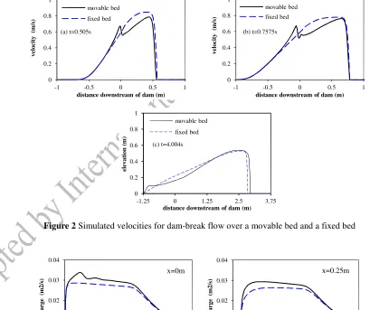
causes the fluid flow to become bulked at the initial stage (e.g., Figure 1a,b). However, the bulking effect becomes weak with the increase of time (Figure 1c,d), because the rheology of the solid phase causes the sediment transport to gradually adapt to the flow. The hydraulic jump around the dam location also vanishes because of the reduction of Froude number. Figure 2 demonstrates the velocity

profiles and it can be seen that the bed scour atx= 0 m causes a hydraulic jump where the flow velocity is increased. Yet the flow velocity at other locations is increased after sediment transport is incorporated. It is also noted that the initial wave front for the movable bed is slightly slower than that over the fixed bed (Figure 2a), but as time increases the wave front with sediment transport is progressively closer to

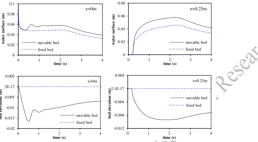
that over the fixed bed (Figure 2b), and then it oversteps the wave front without sediment transport (Figure 2c). This is also manifested by the numerical studies of (Cao et al., 2004; Wu and Wang, 2007). Furthermore, Figure 3 shows the temporal changes of the flow discharge per unit width, the water surface and the bed level for the movable bed and the fixed bed at cross sectionx= 0 m andx= 0.25 m.

Figure 3 indicates that the peak flow for the movable bed and the fixed bed atx= 0 m are 0.0334 m2/s and 0.0293 m2_{/s, respectively, and they are 0.0286 m}2_{/s and 0.0249 m}2_{/s, respectively atx= 0.25 m. The} peak discharge for Scenario 1 with sediment transport is significantly larger than that for Scenario 2 without sediment transport. Similarly, the water surface for the movable bed is also shown to be

Figure 1Measured data and simulated results for dam-break flow over a movable bed and a fixed bed

Figure 2Simulated velocities for dam-break flow over a movable bed and a fixed bed

-0.03 0 0.03 0.06 0.09 0.12

-1 -0.5 0 0.5 1

el evat io n (m )

distance downstream of dam (m)

measured movable bed fixed bed -0.03 0 0.03 0.06 0.09 0.12

-1 -0.5 0 0.5 1

el evat io n (m )

distance downstream of dam (m)

measured movable bed fixed bed -0.03 0 0.03 0.06 0.09 0.12

-1.25 0 1.25 2.5 3.75

el evat io n (m )

distance downstream of dam (m)

movable bed fixed bed -0.03 0 0.03 0.06 0.09 0.12

-1.25 0 1.25 2.5 3.75

el evat io n (m )

distance downstream of dam (m)

movable bed fixed bed 0 0.2 0.4 0.6 0.8 1

-1 -0.5 0 0.5 1

ve lo ci ty (m /s )

distance downstream of dam (m)

movable bed fixed bed 0 0.2 0.4 0.6 0.8 1

-1 -0.5 0 0.5 1

ve lo ci ty (m /s )

distance downstream of dam (m)

movable bed fixed bed 0 0.2 0.4 0.6 0.8 1

-1.25 0 1.25 2.5 3.75

el evat io n (m )

distance downstream of dam (m)

movable bed fixed bed 0 0.01 0.02 0.03 0.04

0 1 2 3 4

d is ch ar ge (m 2/ s) time (s) x=0m movable bed fixed bed 0 0.01 0.02 0.03 0.04

0 1 2 3 4

d is ch ar ge (m 2/ s) time (s) x=0.25m movable bed fixed bed (b) t=0.7575s (a) t=0.505s (d) t=4.004s (c) t=3.003s

(a) t=0.505s (b) t=0.7575s

Figure 3The temporal changes of the simulated flow discharge per unit width, the water surface and the bed level

for dam-break flow over a movable bed and a fixed bed atx= 0 m andx= 0.25 m

4.2. Partial Dam Breach vs Sudden Dam Breach

The flood wave caused by a dam breach is usually a progressive flow-sediment interaction event, not a sudden collapse (Guan et al., 2014; Pickert et al., 2011; Wu et al., 2012). A small-scale experimental event was tested in this section in order to emphasise the blockage effects of sediment

material on flow propagation.

4.2.1 Experimental setup

The experiment conducted by the Université Catholique de Louvain (Spinewine et al., 2004) was used for comparison. The channel flume is 36.2 m long and 3.6 m wide; and a 2.4 m×0.47 m sand dam

was built in the location of 11.8 m in the flume. The upstream and downstream slopes of sand dam are 1:2 and 1:3 respectively. A sand layer of 10 cm is in the downstream, and the bed material is constituted by sand with a median diameter,d50=1.80 mm, specific gravity,s= 2.615, and a loose bed porosity,p= 0.42, after compaction. The upstream reservoir was separated by a gate before which water is stored.

When starting the experiment, the gate was gradually opened so the water filled the second part of the reservoir until the water level was 0.45 m. A small trapezoidal breach was dug on the top middle of the dam to initiate flow overtopping at this point. Subsequently, the breach enlarged with the flow gradually increasing with time. The two blocks besides the sand dike are treated as the part of the sand dam with

the restriction that in the simulation they are not erodible.

4.2.2 Predicted hydrograph

The whole dam and channel are discretised in 2D with x = 0.035 m and y = 0.03 m. The measured data (Spinewine et al., 2004) is used to validate the model. The spatial and temporal evolution

0 0.02 0.04 0.06 0.08 0.1

0 1 2 3 4

w at er su rf ac e (m ) time (s) movable bed fixed bed 0 0.02 0.04 0.06 0.08

0 1 2 3 4

w at er su rf ac e (m ) time (s) movable bed fixed bed -0.02 -0.015 -0.01 -0.005 2E-17 0.005

0 1 2 3 4

b ed el evat io n (m ) time (s) movable bed fixed bed -0.012 -0.008 -0.004 2.1E-17 0.004

0 1 2 3 4

of the entire flood process can be including the outflow hydrograph, evolution of breach size. Manning quantification of flow-induced se

0.019) are used to evaluate the illustrates the comparisons betwe Manning’snchanges the peak va the water level in the reservoir is

model predicts the outflow hydrog good agreement. It was found tha the dam breach as shown in F deposition and wet/dry areas wel

dam and a secondary channel is f

Figure 4Comparisons of the simulate

Figure 5Dam bre

4.2.3 Sediment blockage effects

As previously mentioned, tra whole structure or a constant bre “sudden collapse” hypothesis is sediment material on the outflow

top of dam was also modelled. Th the upper experimental event pre level in the reservoir for ‘sudden

0 15 30 45 60 75

0 1 2

d is ch ar ge (l /s ) tim

be well simulated by the simple and effective mor aph, the peak outflow discharge, the change of water nning’s n has a direct influence on bed shear stres

sediment transport, therefore, three Manning’sn v

he sensitivity in the modelling of the dam breac ween the predicted results and the measured data. It value and the occurrence time of peak outflow disc is also changed. According to the comparisons in Fi

drograph and the temporal change of water level i thatn= 0.018 gave a better prediction of the peak di

Figure 5, the present model reproduces the ch ell; the eroded sediment from the breach primarily

is formed along the centreline.

ulated and measured data: (a) outflow discharge; (b) wate

breach due to flow overtopping at the final equilibrium s

raditionally dam collapse is assumed to be a “sudde breach size. However, such treatments are unrealist is too conservative. In order to demonstrate the ow process, a traditional dam collapse with a consta

he initial breach is assumed as the size at the final previously simulated. Figure 6 shows the outflow dden dam collapse’ and the case with sediment erosion

3 4 5 6

ime (min) measured n=0.017 n=0.018 n=0.019 0 10 20 30 40 50 60

0 1 2 3 4

w at er le ve l (c m ) time (min) measured n=0.017 n=0.018 n=0.019 (a) orphodynamic model, ater level, as well as the ress which decides the values (0.017, 0.018,

ach process. Figure 4 . It can be seen that the ischarge, consequently Figure 4, the proposed

el in the reservoir with k discharge. In terms of characteristic erosion, rily deposits behind the

ater level in the reservoir

stage

udden dam-break” of the listic in reality and the he blockage effects of onstant breach size on the

nal equilibrium stage of ow discharge and water ion and deposition. It is

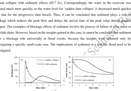
clearly indicated that the existence of sediment blocks the flood propagation significantly, not only in terms of the peak discharge, but also the arrival time. For the ‘sudden collapse’ with a constant breach, the outflow discharge reaches the maximum value (about 212.5 l/s) immediately when the dam-breach occurs, and the peak discharge is significantly over 3 times larger than that with consideration of

gradual collapse with sediment effects (65.7 l/s). Correspondingly, the water in the reservoir was released much more quickly, so the water level for ‘sudden dam collapse’ is decreased much quicker than that for the progressive dam breach. Thus, it can be concluded that sediment plays a role of blockage which reduces the peak flow and delays the arrival time of the peak value during gradual

collapse. The examples of blockage effects of sediment involve the process of failure of river dams or landslide dams. However, based on the insights gained in this case, it cannot be concluded that sediment plays a blockage role universally in flood events, because the insights were obtained only by investigating a specific small-scale case. The implications of sediment in a real-life flood need to be

investigated.

Figure 6Comparison of (a) outflow discharge and (b) water level for the two different conditions of sudden

collapse and gradual collapse with sediment transport

4.3. A Glacial Outburst Flood

4.2.1 Initial model input

A volcano-induced glacial outburst flood occurred unexpectedly at Sólheimajökull, Iceland in July, 1999. This event was well documented and has been physically investigated in detail (Russell et al., 2010). The river channel is located in the south of Iceland and it is about 9 km long and 400-700 m wide.

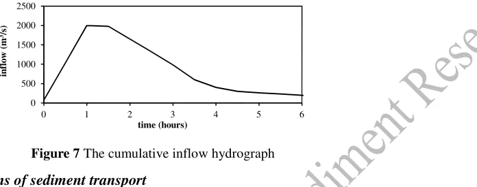
Measurement of pre-flood topography has been made using airborne LiDAR. In this study, the 8 m×8 m resolution of digital elevation model (DEM) data is used as the initial input of bed terrain. The reconstructed flow hydrograph as shown in Figure 7 is used as inflow to the river channel. It can be seen that the inflow is a rapid flash flood event of 6 hours. The base flow is very small in this river channel

before the outburst flood. As the bed elevation at the outlet is about 1-2 m above sea level, and the effects of the seawater on river flood dynamics at the outlet are not significant, it is assumed that the outflow boundary can be set as a free open boundary. Based on the field observations by (Russell et al., 2010), the sediment material is constituted of various grain-size particles from fine granules to coarse

boulders, involving granules (2.8 mm), cobbles (105 mm) and boulders (400 mm) with a density of 0

60 120 180 240

-1 0 1 2 3 4 5 6

d

is

ch

ar

ge

(l

/s

)

time (min)

sudden collapse

with sediment

0 10 20 30 40 50

0 1 2 3 4 5 6

w

at

er

le

ve

l

(c

m

)

time (min)

sudden collapse with sediment

2680 kg/m3. It was assumed that this flood event is mainly dominated by sheet flow load which is conventionally referred to as bed material load transport at high bottom shear stress. To estimate the Manning’s n coefficient, many empirical relationships have been introduced, and in this study, the

Manning’sncoefficient is estimated according to = 0.038 / .

Figure 7The cumulative inflow hydrograph

4.2.2 Multiple implications of sediment transport

In order to ascertain what role sediment transport plays in a large-scale rapid flood event two runs are conducted here: i) clear floodwater modelling without sediment transport; ii) sediment-laden flood modelling with sediment transport. Extensive comparisons between the model outputs from the runs are

performed in terms of both temporal-scale and spatial-scale as follows. For the simulations in this case, the coefficient, =1.0, in the MPM equation was used, and the active layer thickness was set to the median size of bed material following Wu (2004). The values of and the active layer thickness have quantitative impacts on bed erosion and deposition; however, the bed changes and the flood dynamics

are not qualitatively sensitive to the values of the two parameters.

The cross section (x= 332908.86) near the bridge is selected as a typical one as shown in Figure 8(a). The flow hydrographs for the two runs at the typical cross section are shown in Figure 8(b). It clearly indicates that the flow hydrograph is not significantly influenced by the initiation of sediment

transport, as both simulation results have an approximately equivalent value. However, the arrival time of peak discharge for flooding with sediment transport is obviously smaller than that without sediment transport. In other words, the flood propagation is accelerated by sediment transport with approximately 7 minutes acceleration for this flash flood. Moreover, the arrival time of the floodwater front is also

accelerated due to the incorporation of sediment transport. This insight contradicts the understanding obtained from the small-scale flow events previously evaluated. Figure 9 shows the temporal evolution of the water level and the water depth at the gauge (332908.86, 480099.78). It indicates that the water level with sediment transport is smaller than that without sediment transport. However, for the water

depth, the maximum is raised at the peak stage. After about 2.5 hours, the water depth with sediment transport is reduced remarkably. All of these results are attributed to the bed degradation and aggradation caused by the outburst flood. The influence of sediment transport at a specific point cannot represent the effects in the whole river channel. It is necessary to analyse the effects of sediment

transport from the spatial-scale point of view. 0

500 1000 1500 2000 2500

0 1 2 3 4 5 6

in

fl

o

w

(m

3/s

)

Figure 8The temporal

Figure 9The temporal change of the

Figure 10(a) shows the sim incorporation of sediment transpo for both runs differ significantly

smooth contour surface, yet the This is because the high intense ra depressed topography making the surfaces and the water depths for

are reduced because of the cons depths are also decreased in about

Figure 10(a) The contour plot of w

depths and 0 500 1000 1500 2000 2500 0 d is ch ar ge (m 3/s ) 53 54 55 56 57

0 7200 14400 21600

w at er su rf ac e (m ) time (s) with sediment without sediment (a) (b) (a)

ral change of the flow discharge at cross section ofx= 33

the water level, water depth and bed scour at the gauge (3

simulated water depths in the river channel wi nsport at the peak stage, t=2 hours. It is clearly shown

ntly; specifically, the water depth with sediment

he simulated result without sediment transport show e rapid flow scours the protruding bed and re-deposi

the irregular topography smoother. Spatial diffe for both runs are shown in Figure 10(b). It is found

onsideration of sediment transport in 79.9% of the bout 70.7% of the area.

water depths with and without sediment transport; (b) th

nd water surfaces with and without sediment transport

3600 7200 10800 14400 18000 21600

time (s) inflow with sediment without sediment 21600 0 1 2 3 4

0 7200 14400 21600

w at er d ep th (m ) time (s) -1 -0.5 0 0.5 1 1.5 0 7200 b ed sc o u r (m )

= sed- no sed

h=hsed-hno sed

(b)

332908.86

(332908.86, 480099.78)

with and without the n that the water depths nt transport has a very

hows some oscillation. posits the material in the fferences of the water ound that the water levels

the area, and the water

he differences of water

7200 14400 21600

4.2.3 Bed response to rapid flood

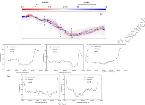
The short-lived outburst flood induces and carries a considerable amount of sediment, causing rapid geomorphic change. The simulated final topography scour is illustrated in Figure 11(a) showing the spatial distribution of the bed erosion and deposition after the flood and five cross sections before and

after the flood. It is found that the erosion and deposition caused by the rapid flash flood mainly occur in the main channel. The erosion and deposition is also found to be more severe in the narrower reach of the river, because the dimensionless bed shear stress is increased in the narrower reach of the river in comparison to that in the wide reach. This induces more sediment into movement and correspondingly,

the sediment load re-deposits within a transport distance. As the inflow discharge is characterized by suddenly increasing to the peak stage and progressively decreasing until 6 hours, the total erosion and deposition volume is closely related to the degree of inflow discharge. It is also noted that the majority of erosion and deposition occurs in approximately 2-3 hours, i.e., the period of peak flow discharge, and

conversely, little scour happens during the falling limb of the hydrograph. The changes of five cross sections due to the rapid flood (cs1-1 to cs5-5) are plotted in Figure 11(b). Intuitively, the cross sections are shown to be smoother compared to the irregular shape before the flood. In order to show the changes of flow conveyance capacity due to bed erosion and deposition, Manning’s equation are used to

estimate the discharge capacity of an open channel following the work in the Fluvial Design Guide (Pepper and Rickard, 2009).

=

/

(16)

where:Qc= discharge capacity (m3/s);A= area of cross section of flow (m2);R=A/P= the hydraulic

radius, (m); P = wetted perimeter of the channel cross section (m); i = hydraulic gradient (usually

approximates to the longitudinal slope of the channel). The term, / , could be considered to be

unchanged before and after the flood. Thus, the changes of the flow conveyance capacity can be approximatelyAandP. Table 1 demonstrates the change ofAR2/3and the net volume of bed changes due to erosion and deposition. It is found that except in cs3-3 the discharge capacity is increased in the other four cross sections along with net erosion. From the full-scale viewpoint, the whole channel bed is

Figure 11(a) The spatial distributio

Table 1 The ch

cross sections

cs1-1 cs2-2 cs3-3 cs4-4 cs5-5 whole channe

5. CONCLUSIONS

In general, floodwater propag with each other. This paper pre sediment transport considering s

effects of sediment transport in simulating both small-scale expe

(b)

tion of geomorphic change during the flood process; (b)

before and after the flood.

changes of hydraulic properties before and after the floo

ons the change of

AR2/3(%)

net volume of

bed changes (m3) explanation

+6.69 140.31 net erosion

+8.22 343.90 net erosion

-7.10 285.45 net deposition

+9.77 727.76 net erosion

+13.90 312.72 net erosion

nel 1.9×105 net erosion

pagates in combination with sediment transport, and presented a 2D layer-based morphodynamic mod ng sheet flow load and different velocities at each

in flood events were extensively analysed and xperimental scenarios and a large-scale glacial outbur

(a)

b) the five cross sections

lood

ion

nd both closely interact odel for non-uniform ch layer. The multiple

nd emphasised through outburst flood. It is noted

that the effects of sediment transport are multiple depending on the real circumstances of flood events. The results clarify the insights on the interactions of flow and sediment transport quantitatively from the viewpoint of numerical modelling. The comparisons and analysis of the modelling results indicate that: (1) For events such as dam-break flows over flat movable beds, peak flow discharge, water surface

elevation and water depth are increased because of the consideration of sediment transport even though movable bed is severely scoured. The velocity of the wave front is initially slowed down by sediment entrainment, yet it gets faster after the solid phase adapts to the flow, which leads to a faster wave front in comparison with dam-break flow over a fixed bed.

(2) For events such as flow over natural dams or river embankments, erosion of sediment material delays the onset of the flood, changing the hydrograph of the flow compared to the assumption of ‘sudden dam collapse’.

(3) During rapid outburst floods over a natural river channel, morphological changes lead to net

erosion. The flow conveyance capacity of the river channel is increased along with an increase of flow area. Also, sediment entrainment increases the mass of the sediment-water mixture. The inclusion of sediment transport and morphological changes has significant impacts on flood dynamics: floodwater propagation is accelerated, water levels are mostly reduced, but

water depths are decreased for the most part in the river channel. In response to the outburst flood, the majority of bed changes occur during the rising limb of the hydrograph, and it is more severe in the narrower reach of the river. The findings from a real-world flood extend and improve the understanding previously gained in the case of small-scale idealised dam-break

flows over a movable bed. It is clear how flood dynamics are influenced is dependent on the flood-induced morphological changes.

Flood inundation cannot just focus solely on the water flow and it is necessary to incorporate the effects of sediment transport. The understanding in this study is obtained based on testing a couple of

small-scale events and a large-scale glacial outburst flood. However, understanding might be further improved by testing multiple types of real-world events, such as floods with only bed erosion or only deposition.

ACKNOWLEDGEMENT

We wish to thank Dr. Jonathan Carrivick from the School of Geography, University of Leeds for providing the data on the glacial outburst flood.

REFERENCE

Abderrezzak, K.E., Paquier, A., 2011. Applicability of sediment transport capacity formulas to dam-break flows over movable beds. Journal of Hydraulic Engineering, 137(2), 209-221.

Jökulsá á Fjöllum, NE Iceland. Quaternary Science Reviews, 24(22), 2319-2334.

Cao, Z., Pender, G., Wallis, S., Carling, P., 2004. Computational dam-break hydraulics over erodible sediment bed. Journal of Hydraulic Engineering, 130(7), 689-703.

Capart, H., Young, D.L., 1998. Formation of a jump by the dam-break wave over a granular bed. Journal of Fluid Mechanics, 372, 165-187.

Carrivick, J.L., Jones, R., Keevil, G., 2011. Experimental insights on geomorphological processes within dam break outburst floods. Journal of Hydrology, 408(1–2), 153-163.

Carrivick, J.L., Manville, V., Graettinger, A., Cronin, S.J., 2010. Coupled fluid dynamics-sediment transport modelling of a Crater Lake break-out lahar: Mt. Ruapehu, New Zealand. Journal of Hydrology, 388(3-4), 399-413.

Carrivick, J.L., Rushmer, E.L., 2006. Understanding high-magnitude outburst floods. Geology Today, 22(2), 60-65.

Fraccarollo, L., Capart, H., 2002. Riemann wave description of erosional dam-break flows. Journal of Fluid Mechanics, 461, 183-228.

Greimann, B., Lai, Y., Huang, J.C., 2008. Two-dimensional total sediment load model equations. Journal of Hydraulic Engineering, 134(8), 1142-1146.

Guan, M., Wright, N., Sleigh, P., 2014. 2D process-based morphodynamic model for flooding by noncohesive dyke breach. Journal of Hydraulic Engineering, 140(7), 04014022.

Guan, M.F., Wright, N.G., Sleigh, P.A., 2013. A robust 2D shallow water model for solving flow over complex topography using homogenous flux method. International Journal for Numerical Methods in Fluids, 73(3), 225-249.

Li, S., Duffy, C.J., 2011. Fully coupled approach to modeling shallow water flow, sediment transport, and bed evolution in rivers. Water Resources Research, 47(3), W03508.

Li, W., van Maren, D.S., Wang, Z.B., de Vriend, H.J., Wu, B., 2014. Peak discharge increase in hyperconcentrated floods. Advances in Water Resources, 67, 65-77.

Manville, V., White, J.D.L., Houghton, B.F., Wilson, C.J.N., 1999. Paleohydrology and sedimentology of a post-1.8 ka breakout flood from intracaldera Lake Taupo, North Island, New Zealand. Geological Society of America Bulletin, 111(10), 1435-1447.

Meyer-Peter, E., Müller, R., 1948. Formulas for bed load transport, Proceedings, 3rd_{IAHR World Congress,}

Stockholm, Sweden, 39-64.

Nielsen, P., 1992. Coastal bottom boundary layers and sediment transport. Advanced Series on Ocean Engineering, 4. World Scientific.

Pepper, A., Rickard, C., 2009. Works in the river channel, availible at http://evidence.environment-agency.gov.uk /FCERM/Libraries/Fluvial_Documents/Fluvial_Design_Guide_-_Chapter_8.sflb.ashx.

Pickert, G., Weitbrecht, V., Bieberstein, A., 2011. Breaching of overtopped river embankments controlled by apparent cohesion. Journal of Hydraulic Research, 49(2), 143-156.

Russell, A.J., Tweed, F.S., Roberts, M.J., Harris, T.D., Gudmundsson, M.T., Knudsen, Ó., Marren, P.M., 2010. An unusual jökulhlaup resulting from subglacial volcanism, Sólheimajökull, Iceland. Quaternary Science Reviews, 29(11–12), 1363-1381.

Simpson, G., Castelltort, S., 2006. Coupled model of surface water flow, sediment transport and morphological evolution. Computers & Geosciences, 32(10), 1600-1614.

Smart, G., Jäggi, M., 1983. Sediment transport on steep slopes. Mitteilung. 64. Versuchsanstalt fu¨ r Wasserbau, Hydrologie und Glaziologie, ETH Zurich, Zurich.

UK.

Spinewine, B., Capart, H., 2013. Intense bed-load due to a sudden dam-break. Journal of Fluid Mechanics, 731, 579-614.

Spinewine, B., Delobbe, A., Elslander, L., Zech, Y., 2004. Experimental investigation of the breach growth process in sand dikes, Proceedings, Second International Conference on Fluvial Hydraulics, Napoli, Italy, 983–991.

Toro, E.F., 2001. Shock-Capturing Methods for Free-Surface Shallow Flows, John Wiley&Sons, LTD, Chichester, UK.

Wong, J.S., Freer, J.E., Bates, P.D., Sear, D.A., Stephens, E.M., 2014. Sensitivity of a hydraulic model to channel erosion uncertainty during extreme flooding. Hydrological Processes.

Wu, W., 2004. Depth-Averaged Two-dimensional numerical modeling of unsteady flow and nonuniform sediment transport in open channels. Journal of Hydraulic Engineering, 130(10), 1013-1024.

Wu, W., Marsooli, R., He, Z., 2012. Depth-averaged two-dimensional model of unsteady flow and sediment transport due to noncohesive embankment break/breaching. Journal of Hydraulic Engineering, 138(6), 503-516.

Wu, W.M., Wang, S.S.Y., 2007. One-dimensional modeling of dam-break flow over movable beds. Journal of Hydraulic Engineering, 133(1), 48-58.

Xia, J., Lin, B., Falconer, R.A., Wang, G., 2010. Modelling dam-break flows over mobile beds using a 2D coupled approach. Advances in Water Resources, 33(2), 171-183.

Zech, Y., Soares-Frazão, S., 2007. Dam-break flow experiments and real-case data. A database from the European IMPACT research. Journal of Hydraulic Research, 45(sup1), 5-7.