Disaggregate path flow estimation in an iterated DTA microsimulation

This is a repository copy of Disaggregate path flow estimation in an iterated DTA microsimulation.

White Rose Research Online URL for this paper: http://eprints.whiterose.ac.uk/85162/

Version: Accepted Version

Article:

Flotterod, G and Liu, R (2014) Disaggregate path flow estimation in an iterated DTA microsimulation. Journal of Intelligent Transportation Systems: Technology, Planning, and Operations, 18 (2). 204 - 214. ISSN 1547-2450

https://doi.org/10.1080/15472450.2013.806854

[email protected] https://eprints.whiterose.ac.uk/

Reuse

Unless indicated otherwise, fulltext items are protected by copyright with all rights reserved. The copyright exception in section 29 of the Copyright, Designs and Patents Act 1988 allows the making of a single copy solely for the purpose of non-commercial research or private study within the limits of fair dealing. The publisher or other rights-holder may allow further reproduction and re-use of this version - refer to the White Rose Research Online record for this item. Where records identify the publisher as the copyright holder, users can verify any specific terms of use on the publisher’s website.

Takedown

If you consider content in White Rose Research Online to be in breach of UK law, please notify us by

Flötteröd, G. and Liu, R (2014) Disaggregate path flow estimation in an iterated DTA microsimulation. Journal of Intelligent Transportation Systems: Technology, Planning and

Operations. Vol 18(2), 204-214. DOI:10.1080/15472450.2013.806854

Disaggregate path flow estimation in an iterated DTA

microsimulation

Gunnar Flötteröd

KTH Royal Institute of Technology

Department of Transport Science

Teknikringen 72, 11428 Stockholm, Sweden

[email protected] (corresponding author)

Ronghui Liu

Institute for Transport Studies

University of Leeds

Leeds LS2 9JT, England,

[email protected]

Abstract

This text describes the first application of a novel path flow and origin/destination (OD)

matrix estimator for iterated dynamic traffic assignment (DTA) microsimulations. The

presented approach, which operates on a trip-based demand representation, is derived from an

agent-based DTA calibration methodology that relies on an activity-based demand model

(Flötteröd et al., 2011a). The objective of this work is to demonstrate the transferability of the

The calibration (i) operates at the same disaggregate level as the microsimulation and (ii) has

drastic computational advantages over conventional OD matrix estimators in that the demand

adjustments are conducted within the iterative loop of the DTA microsimulation, which

results in a running time of the calibration that is in the same order of magnitude as a plain

simulation. We describe an application of this methodology to the trip-based DRACULA

microsimulation and present an illustrative example that clarifies its capabilities.

1 Introduction

This section introduces a novel path flow and origin/destination (OD) matrix estimator

for iterated dynamic traffic assignment (DTA) microsimulations. The first part of this

introduction describes the basic concepts of these simulations and reviews some of the

existing implementations. The second part revisits existing OD matrix and path flow

estimators. Based on this review, the new approach is then motivated.

Iterated DTA microsimulations are characterized by the following features. They are

microscopic in that both travelers and vehicles are modeled at the disaggregate level. They are

iterative in that the simulation runs typically according to the logic outlined in Algorithm 1,

where a demand simulator and a supply simulator are alternately executed until a state of

mutual consistency is reached. Finally, they are usually stochastic in that at least the simulated

travel behavior is non-deterministic, whereas the traffic flow model may be either

deterministic or stochastic. The foundations of the iterated simulation approach have been laid

by Cascetta (1989) and Cascetta and Cantarella (1991), and their application to increasingly

complex model systems is still the topic of ongoing research (Nagel et al., 1998; Nagel and

Algorithm 1 leaves open which behavioral dimensions are represented by the demand

simulation (e.g., route choice, departure time choice, destination choice, mode choice, ect),

and, indeed, the iterative approach can in principle cope with any of these dimensions (Nagel

and Flötteröd, 2012). However, only few existing DTA microsimulations go beyond route

choice adjustments; amongst them are DynaMIT (Ben-Akiva et al., 1998; DynaMIT, accessed

2011), METROPOLIS (De Palma and Marchal, 2002), and DRACULA (Liu, 2005;

DRACULA, accessed 2011) which also adjusts departure time choice for independent trips,

and MATSim (Nagel et al., accessed 2011; Nagel and Flötteröd, 2012; Raney and Nagel,

2006) which in its current implementation adjusts route, departure time, and mode choice for

complete trip chains and is continuously being extended towards further demand dimensions

(Horni et al., 2008). Far more common are iterated microsimulations that constrain

themselves to the equilibration of route choice (and a strictly trip-based demand

representation). Amongst those are AIMSUN (TSS Transport Simulation Systems, 2006,

accessed 2011), DYNAMEQ (INRO, accessed 2011), and PARAMICS (Quadstone Paramics

Ltd., accessed 2011).

The usual representation of a trip-based demand is a (possibly time-dependent) OD

matrix that describes the number of trips from every origin zone to every destination zone in a Algorithm 1 Iterated DTA microsimulation

1. Initialization. Give every traveler an initial perception of the conditions in the

network.

2. Iterations. Repeat the following until stationary conditions are reached.

a. Demand simulation. Travelers select new mobility plans based on what

they have observed during previous iterations.

b. Supply simulation. The mobility plans of all travelers are simultaneously

traffic network. The traditional OD matrix estimation problem is to estimate an OD matrix

from traffic counts on network links and supplementary prior information. In lightly

congested conditions, link flows are linear combinations of path flows, yielding a

mathematically convenient setting, in which OD matrix estimation techniques such as entropy

maximization and information minimization (van Zuylen and Willumsen, 1980), Bayesian

estimation (Maher, 1983), generalized least squares (Bell, 1991; Bierlaire and Toint, 1995;

Cascetta, 1984), and maximum likelihood estimation (Spiess, 1987) have been applied. These

methods can be carried over at least approximately to congested networks (Maher et al., 2001;

Yang, 1995; Yang et al., 1992; Bierlaire and Crittin, 2006; Cascetta and Posterino, 2001). The

further addition of a time dimension, yielding various dynamic OD estimators, is also possible

(Cascetta et al., 1993; Ashok, 1996; Bierlaire, 2002; Sherali and Park, 2001; Zhou, 2004).

All of the above-mentioned demand estimators adjust OD matrices subject to a given

route choice model that is embedded in the traffic assignment procedure. Since route choice

modeling is an intricate task (Frejinger, 2008), modeling errors are likely to introduce biases

in the estimated OD matrices. This problem can be avoided through the use of path flow

estimators (PFEs). The first PFE, introduced by Bell (1995) and Bell et al. (1997), estimates

static path flows from link volume measurements based on a multinomial logit stochastic user

equilibrium (SUE) modeling assumption. Further developments along these lines allow for

multiple user classes and simplified traffic flow dynamics (Bell et al., 1996) as well as for the

incorporation of a deterministic user equilibrium (UE) modeling assumption (Sherali et al.,

2003, 1994; Nie and Lee, 2002; Nie et al., 2005). Summing up the path flows between an OD

pair yields its OD flow, which means that PFEs also estimate OD flows.

The new path flow and OD matrix estimator described in this work operates on a

trip-based demand representation, but it is derived from an agent-based DTA calibration

approach is mathematically developed in Flötteröd et al. (2011a), and its applicability for

large, real scenarios is demonstrated in Flötteröd et al. (2011b). The objective of this work is

to demonstrate the transferability of the agent-based approach to the more widely used OD

matrix-based demand representation. This complements previous presentations, where this

possibility is stated but not made concrete. Here, it is shown in terms of an operational

example how the new approach can be deployed for the estimation of OD matrices and path

flows in a microsimulation context. The used calibration software is freely available on the

Internet (Flötteröd, accessed 2011).

Transferring the originally agent-based approach to the OD/path flow domain also carries

over its advantages to this domain. The new approach goes beyond existing methods in that it

• estimates the trip-making of individually simulated travelers without any aggregation;

• is compatible with almost arbitrary demand and supply simulators; and

• has a computational complexity that is in the order of a plain simulation.

The reduction of an activity-based approach into the trip-based approach described in this

article is possible because a trip constitutes a subset of a trip chain, and a trip chain constitutes

the mobility-related side of an all-day travel and activity plan. Since the activity-based

calibration approach adjusts all-day travel plans to traffic counts, it is also applicable to the

basic case of travel plans consisting only of a single trip. The essential difference to all other

PFEs presented in the literature is that the presented approach does not aggregate

travelers/trip-makers into continuous flows but treats them as integer entities, consistently

with the individual representation of trip-makers in a microscopic DTA simulation.

This work is of particular relevance for Intelligent Transportation Systems (ITS).

Agent-based simulations of activity-based models may be computationally too heavy to be

deployed in real-time contexts, and hence the corresponding calibration methodology was so

Flötteröd (2008)). OD matrices and paths may be more suited for short-term and real-time

demand estimation, such that an operation transferral of the activity-based methodology to

these datastructures, as presented in this article, is likely to contribute to the real-time

monitoring of traffic conditions in ITS applications.

The remainder of this article is organized as follows. Section 2 introduces the two

software systems deployed in this study: the DRACULA microsimulation and the Cadyts

calibration tool, which implements the proposed methodology. A case study that clarifies the

workings of the new approach is given and discussed in Section 3. Finally, the article is

concluded in Section 4, and ongoing and future research work is described.

2 Framework and system components

The work presented in this article involves two software systems: the DRACULA

microsimulation and the Cadyts calibration tool. This section describes these systems and

their interactions. DRACULA is outlined in Subsection 2.1, and Cadyts is introduced in

Subsection 2.2. The interaction of both systems is described in Subsection 2.3.

2.1 DRACULA

–

a microscopic simulation DTA model

DRACULA (“Dynamic Route Assignment Combining User Learning and

microsimulAtion”) is a simulation tool to investigate the dynamics of demand and supply

interactions in road networks. The emphasis is on the integrated microsimulation of individual

trip-makers’ decisions, travel experiences, and learning. DRACULA complies with the

simulation structure given in Algorithm 1.

The system explicitly models individuals’ day-to-day route and departure time choices,

and how their past experience and knowledge of the network influence their future choices.

lane-changing rules. The system evolves continuously from one day to the next until a

pre-defined number of days or a broadly balanced state between the demand and supply is

reached. Simulation results can be obtained throughout the evolution and on not just the

means but also variances and probability distributions both within-day and between days. The

full details of the DRACULA suite of models and their applications have been reported

elsewhere (e.g., Hollander and Liu, 2008; Liu et al., 2006; Liu and Tate, 2004; Panis et al.,

2006) and will therefore not be detailed herein.

For the purposes of this article, DRACULA’s sophisticated supply simulator is coupled

with a simple, externally implemented multinomial logit (MNL) route choice model

(Ben-Akiva and Lerman, 1985), and departure time choice is neglected (in that fixed

departure times are assumed). The limitations of MNL route choice models, in particular with

respect to route overlap, are well understood and can to some extent be corrected for without

abstaining from the MNL’s convenient functional form (Ben-Akiva and Bierlaire, 2003;

Cascetta et al., 1996). However, the synthetic study presented in this article is sufficiently

served by a plain MNL model.

Formally, denote a single trip-maker by n and its choice set of available routes by C . _n

The probability P i that n chooses route n( ) iCn follows a multinomial logit model









exp ( )

( )

exp ( )

n n n n j C V i P i V j    



where V i is the systematic utility of alternative _n( ) i as perceived by n , and  is a scale

parameter. Letting 0 results in a choice model that is insensitive to utility and hence

predicts a uniform choice distribution, whereas for   only the alternative of maximum systematic utility is selected with positive probability. In all experiments, V i is set to the n( )

negative travel time one would have experienced on the considered route in the previous

for long-term driver memories with different weights on different days) are not exploited in

this study. Further investigations with more complex modeling assumptions are left as a topic

for future research.

The dynamics of the traffic assignment problem are comprised in this notation as follows:

• A time-dependent assignment problem requires to model path choice probabilities per

time slice. In such a setting, the model (1) is applied per time slice, and the utility

evaluated in this model is also computed time-dependently.

• Further choice dimensions can be incorporated in this notation by re-defining the

elements in the choice sets as tuples of choices. For example, adding departure time

would turn the elements of C into (route, departure time) tuples. _n

The simplicity of the used notation reflects the flexibility of the calibration approach. As

long as there are trip-makers, (possibly time-dependent) utilities of alternatives, probabilistic

choice models, and (possibly time-dependent) traffic counts, the presented approach is

applicable.

Variability in the total demand levels is enabled by giving every replanning trip-maker an

additional empty route that represents the alternative of not making a trip. Assuming a total

number of N trip makers for a given OD pair (and departure time interval) and assuming

that on average a fraction of f(0,1) trip makers actually travels per day gives the no-travel

route a choice probability of 1 f and requires to scale down the choice probabilities of all

other routes by f . This turns the daily demand for the given OD pair into a binomial random

variable with mean fN and variance Nf(1 f). Although the stay-at-home alternative has

(again for simplicity) a fixed probability to be chosen, it can be formally accounted for within

(1) by solving exp[ (stay-at-home)] 1 exp[ (stay-at-home)] exp[ ( )]

n

n

n n

j C V

f

V V j



 



 

1 1 1

(stay-at-home) ln ln exp[ ( )]

n

n n

j C

f

V V j

f 

  

 

  

 _{ } _{ }

  



where the logsum term is computed only over the true route choice alternatives. Whenever the

following text speaks of route choice according to (1), this therefore comprises the additional

no-trip alternative.

2.2 Cadyts

–

Calibration of dynamic traffic simulations

Cadyts (“Calibration of dynamic traffic simulations”; Flötteröd, 2009; accessed 2011) is a

continuously developed software toolbox that allows to estimate activity based travel demand

models from traffic counts and vehicle re-identification data. Cadyts has been originally

developed for the calibration of agent-based DTA simulations, which do not use OD matrices.

In this subsection, a more specific perspective is adopted on a trip-based demand

representation with route choice and dropping a trip being the only choice dimensions.

For the sake of clarity, a somewhat simplified calibration setting is described in the

following, which results in a particularly interpretable formulation of the estimation: (i) the

network is assumed to be uncongested, (ii) the demand simulator is assumed to deploy an

MNL route choice model, (iii) the traffic count sensors are assumed to have univariate normal

error distributions, and (iv) the objective is to estimate the output (choice distribution) of the

demand model, not its parameters. See Flötteröd et al. (2011b) for a straightforward

derivation of these assumptions from the general approach; some explanation given in that

reference are summarized in this subsection.

Denote by y the traffic count obtained on link a in time interval _ak k, by _ak2 the respective sensor’s error variance, and by A the set of all sensor-equipped links. The

simulated counterpart of a measurement y_ak is denoted by q_ak . This quantity is

straightforwardly obtained from DRACULA by counting the number of simulated vehicles

in a Bayesian framework, where, essentially, the prior route choice distribution P i of (1) is _n( )

combined with the measurements’ likelihood function into a posterior route choice

distribution P i_n( |{y_{ak a A k}}_{ ,} ) given the sensor data. Under the above assumptions, the

following approximation of the posterior distribution can be obtained:

2 , ; ~

,

2 , ; ~ exp ( )

( | { } )

exp ( )

n

ak ak n _{a A k ak i}

ak n ak a A k

ak ak n

j C a A k ak j

ak

y q

V i

P i y

y q V j          _               







where ak~i indicates that the network travel times are such that following route i, for a

given departure time, implies crossing the sensor on link a during simulation time step k.

Equation (3) is obtained from a consistent mathematical derivation (Flötteröd et al., 2011a),

but it also has a clear intuitive meaning.

The prior route choice probabilities are changed only through additive modifications of

the utilities. That is, the only affected elements of the behavioral model are the

alternative-specific constants (ASCs). This is plausible: the objective in the given setting is to

adjust the choices and not the choice model coefficients, and an ASC captures all effects on a

choice that are not reflected by the attributes of the alternatives (Ben-Akiva and Lerman,

1985).

Regarding the nature of the ASC modifications, consider a single addend (y_akq_ak) /_ak2

in the utility correction. If more vehicles are counted in reality than are simulated (yak qak),

the addend is positive and the utility of routes that cross the sensor on link a in time interval

k is increased. Hence, simulated drivers are encouraged to select routes that contribute to the

simulated count, which results in a lower deviation between reality and simulation. If, on the

other hand, the simulation generates a flow that is higher than the real count (y_akq_ak), the

contribute to q . The scaling of the utility corrections by _ak 2

1/_ak ensures that more reliable

sensors take greater effect than unreliable ones. In summary, the calibration works like a

controller that steers the simulated drivers towards a reasonable fulfillment of the sensor data.

That is, the estimator (3) calibrates simulated behavior, but it does not calibrate the underlying

choice model parameters, such as f or  in (2) This is exactly the type of problem also

tackled by an OD or path flow estimator, which does not explain why travelers select

particular routes, destinations or departure times, but only estimates this behavior as such.

Like in the OD matrix estimation problem, the amount of information that can be

extracted from (possibly time-dependent) traffic counts is limited, and supplementary

information is needed in order to state a well-posed estimation problem. The present

formulation solves this problem differently from traditional approaches in that the DTA

simulator itself constitutes the prior information. Even in the extreme case of observing no

traffic counts at all, the additive utility corrections in (3) become zero and the calibration falls

back to a plain simulation. That is, the approach functions with arbitrarily small amounts of

sensor data. However, it also needs to be acknowledged that using a limited amount of data

also reveals only a limited amount of information, and hence one is just as dependent on, e.g.,

carefully selected sensor locations as in the traditional OD matrix estimation problem.

In the traditional OD matrix estimation problem, an over-fitting to the sensor data is

avoided by carefully selecting the weights assigned to the sensor data and to the prior

information, e.g., in terms of inverse covariance matrices (Cascetta, 1984). The estimator

described here also incorporates such a balancing mechanism, where the “weighting

parameters” are the sensor data’s standard deviation  in (3), the scale parameter  in (1), and the traveling probability f in (2): The larger , the lower the utility correction in (3). The larger  , the less the choice model (1) is spread out across alternatives, reflecting

closer f is to one, the less attractive becomes the stay-at-home alternative in (2), meaning

that the analyst is increasingly confident about the total demand level.

Cadyts can cope with more general settings than what is presented here. For example, the

experiments described in Section 3 rely on some additional features of the calibration that

enable its application in congested conditions (Flötteröd and Bierlaire, 2009).

2.3 Integration of DRACULA and Cadyts

This section describes how DRACULA and Cadyts are linked together. The next section

then deploys the technology described here for a series of experiments.

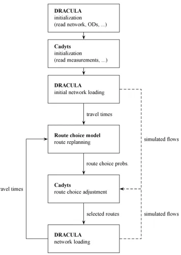
The communication between DRACULA and Cadyts is based on exchanging data

through files. The flow chart of Figure Error! Reference source not found. outlines the

interactions between the two systems. The program logic is implemented in a Python script

Figure 1: Interactions between DRACULA and Cadyts. The program flow is along the solid

After an initialization of both systems, DRACULA is executed once with an arbitrarily

selected route for each traveler. Hereafter, the iterations start. Given the most recent travel

times, the route choice model is evaluated for every single traveler, and the resulting prior

route choice probabilities are stored (recall that this includes the option of not making a trip).

This corresponds to an evaluation of (1). Cadyts then internally adjusts the route choice

probabilities according to (3), samples one route per trip-maker from the resulting posterior

distribution, and saves this route as the chosen alternative. DRACULA then loads all chosen

routes on the network. The resulting travel times are fed back to the route choice model, and

the iterations start anew.

Cadyts operates at the fully disaggregate level in that it deals with individual travelers

(trip makers) without associated OD pairs. The demand representation in DRACULA is based

on OD matrices (possibly separated by time slice and/or user class). In order to interact these

two approaches, DRACULA samples a population of trip-makers from the OD matrices in its

initialization step. Every trip-maker in this population is then maintained as a uniquely

identified entity throughout all following process steps, and its association to one particular

OD pair is also stored. This allows to re-aggregate estimated path flows and OD matrices

from the individually adjusted route choice behavior.

3 Experiments

We investigate the interactions of the Cadyts calibration with the DRACULA simulation

in a synthetic scenario. The purpose of these experiments is to clarify the functioning and the

capabilities of the approach. Experiments with real networks are the subject of future

research. The computational feasibility of the calibration methodology for large-scale

scenarios is demonstrated in Flötteröd et al. (2011b), where, however, a multi-agent

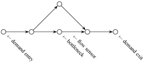
The experiments are run in the network shown in Figure 2. Demand enters the network at

the leftmost node, turns either left or goes straight at the diverge, and leaves the network at the

rightmost node. A traffic light is located in the center of the straight route, serving as a

bottleneck that generates congestion-dependent travel times. The link capacities and

geometrical layouts are chosen such that the traffic light constitutes the only bottleneck in the

system, and that free-flow travel is possible everywhere else. The two routes differ by 23

seconds under free-flow conditions (taking into account an average delay due to the signal)

and by 1 km in length. One may think of a straight route going through a city-center and of a

longer by-pass route. The difference in free-flow travel times corresponds to approximately

17 % of the free-flow travel time on the straight route.

Figure 2: Test network

In this experiment, a population of 3000 drivers is considered. The stay-at-home probability

1 f is set to 1/3 in (2), which means that on average 2000 travelers decide to make a trip,

with a standard deviation of approximately 26 travelers. The scale parameter  of the utility

function (negative travel time) in the logit choice model (1) is set to 0.01. Time is given in

seconds. This results in the following overall form of the utility function:

 













if is a route ( )

100 ln 1/ 2 100 exp 0.01 exp 0.01 if is stay-at-home

i n

t i

V i

t t i

 

  _{   }

where the second row results form an insertion of the concrete parameter values for  and

f into (2). Considering both routes and the stay-at-home option, the choice set is hence

three-dimensional. The length of the analysis period is one hour, an the demand is distributed

uniformly over this time interval.

All calibration experiments follow the logic outlined in Figure 1. Plain simulations are

conducted by taking Cadyts out of the loop, which is the same as running the calibration with

an empty measurement file, i.e., with A{} in (3). All simulations and calibrations are run

for 100 iterations, which appears sufficient to reach stationary conditions by visual inspection

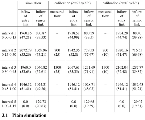
Table 1: Test results. Time intervals are written as “hours:minutes”, all other values are

vehicles per hour (veh/h).

simulation calibration ( =25 veh/h) calibration ( =10 veh/h)

inflow of entry link inflow of sensor link measured flow inflow of entry link inflow of sensor link measured flow inflow of entry link inflow of sensor link interval 1 0:00-0:15 1960.16 (47.21) 880.87 (39.53) – 1938.51 (44.99) 880.39 (39.5) – 1934.28 (44.74) 880.0 (39.88) interval 2 0:15-0:30 2072.79 (53.26) 1069.96 (53.21) 700 (25) 1942.35 (52.8) 779.53 (57.67) 700 (10) 1920.16 (51.47) 716.55 (66.68) interval 3 0:30-0:45 1960.0 (53.63) 1046.82 (52.61) 1300 (25) 2067.61 (55.35) 1231.69 (71.91) 1300 (10) 2102.04 (52.48) 1287.77 (89.32) interval 4 0:45-1:00 1946.12 (51.41) 1024.31 (49.26) – 1946.12 (51.41) 1028.71 (48.03) – 1946.12 (51.41) 1032.63 (51.21) interval 5 1:00-1:15 0.0 (0.0) 129.73 (20.63) – 0.0 (0.0) 129.65 (19.39) – 0.0 (0.0) 129.02 (19.31)

3.1 Plain simulation

A plain simulation in this setting results in the demand levels and simulated traffic counts

indicated in the first wide column (“simulation”) of Table 1. Every field of this table displays

two values: a mean value and a standard deviation (in brackets). All statistics are obtained

from the last 50 iterations of the respective runs.

The first simulation column displays the network entry flows. Their mean values are

consistent with the demand profile. Their standard deviations are higher than the 26 veh/h one

would expect from the binomial demand distribution, which is most likely a result of the link

after one hour, which means that no demand is held back at the network entry because of

congestion effects.

The second simulation column displays the simulated flows at the measurement location.

Roughly half of the total network entries take the straight route (and hence pass the sensor

location). Because it takes some time to reach the sensor link from the network entry, vehicles

enter the sensor link even after one hour. This effect is compounded by the traffic light right

upstream of the sensor link, which generates an additional delay for vehicles that take the

straight route.

Figures Figure 3 and Figure 4 show the evolution of the network and sensor link inflows

for two representative 15-min time interval over the iterations of the simulation. Since the

initial route assignment is a 50/50 split, the system stabilizes almost immediately around a

stationary distribution. The ongoing variability in the curves is due to (i) demand level

fluctuations, (ii) route choice variations, and (iii) stochastic traffic flow dynamics.

Figure 4: Sensor link inflows [veh/h] over iterations of plain simulation

3.2 Calibration

The same one-hour peak period as before is considered, where the traffic counts (which

are arbitrarily constructed only in order to demonstrate the workings of the approach) are

given in four 15 min time intervals. We investigate the exploitation of this sensor data to the

adjustment of both the route choice and the total demand levels across all time slices. (Note

that the estimation takes place jointly for all time slices.) In summary, the calibrated

simulation adjusts to the measurements according to Algorithm 2 (which constitutes a

The second and third main column of Table 1 show the results of two calibration

experiments. In both experiments, the same measurement data is used: a measured flow that is

roughly 300 veh/h lower than the plain simulation in the second time interval, and a measured

flow that is roughly 300 veh/h higher than the plain simulation result in the third time interval.

Through this, we investigate the ability of the calibration to both increase and decrease

demand and path flow levels. No measurements are assumed to be available in the first and

fourth time interval in order to underline that the method functions with arbitrarily few

measurements. The two experiments differ in the standard deviation of the hypothetical sensor

data, which is 25 veh/h in the first calibration experiment (second main column) and 10 veh/h

in the second one (third main column).

In a nutshell, the calibration yields the effect one would expect from the sensor data: it

modifies both the demand levels and the route choice in a way that improves the measurement

reproduction, with the fit improving as the variance of the sensor data is reduced. This is

plausible in that the calibration is designed to generate a statistically consistent combination

of the prior information contained in the model system and the additional information

contained in the sensor data.

Algorithm 2 Iterated DTA microsimulation

1. Initialization. Give every traveler an initial perception of the conditions in the

network.

2. Iterations. Repeat the following until stationary conditions are reached.

a. Calibrated demand simulation. Trip-makers select new trips (or decide to

stay at home) based on Error! Reference source not found., using utilities

as defined in Error! Reference source not found..

Supplementary to Table 1, Figures Figure 5 and Figure 6 give the evolution of the

calibrated network entry and sensor link entry flows over the iterations. Based on these

figures and Table 1, three further observations can be made.

Figure 5: Network entries [veh/h] over iterations of calibration experiment 2 ( =10 veh/h)

Figure 6: Sensor link inflows [veh/h] over iterations of calibration experiment 2 ( =10 veh/h)

First, the adjustment of the demand levels is not as prominent as that of the route flows.

This is due to the behavioral distribution generated by the simulation system (without any

the relative variability in the route flows is higher than the variability in the demand levels.

Arguing in Bayesian terms (from which the calibration is indeed derived), this leaves greater

freedom for adjustments of the prior route choice distribution than for adjustments of the prior

demand level distribution, and hence the route flows are affected more strongly than the total

demand levels by the sensor data.

Second, the variability in the sensor link entry flows increases as the fit to the

measurements is increased. This is so because the measurements are selected to represent

out-of-equilibrium conditions (they differ substantially from the flows resulting from a plain

simulation): as the system is moved out of equilibrium, its sensitivity to the

bottleneck-induced delay on the straight route increases, hence the reaction of the route choice

model becomes stronger, and variability increases. This means that, although the calibration

only compares mean simulated and measured flows, it implicitly also adjusts the system

variability in a plausible way.

Third, the calibrated simulation attains quite rapidly a stationary state. Noting that the

behavioral adjustment process implemented by the calibration is embedded within the

iterative loop of the simulation, this indicates a vast computational advantage over usual

approaches where the iterative simulation is embedded within an outer adjustment loop of the

OD matrix. (The path flow estimator by Bell also is a one-step estimator, but it is yet to be

transferred to a microsimulation setting.) In the presented approach, no outer loop is present,

and the complexity of a calibration is in the order of a plain simulation: The computational

overhead of the calibration is limited to (i) calculating one utility addend per traffic count and

(ii) adding these numbers to the utilities of the alternatives each trip maker faces, cf. (3). The

memory complexity of the calibration is limited to storing these utility addends. Other

calibration is limited to a few percent of the total running time (Flötteröd et al., 2011a,

2011b).

Clearly, these results are conditional on the information obtainable with a single sensor.

Given that two only loosely couple path flows are to be estimated, one would expect a

supplementary sensor either on the detour link or at the network entry to provide more precise

estimates. In general, any sensor location strategy applicable to standard OD matrix

estimators can be deployed here as well.

4 Summary and outlook

This paper describes the first application of a novel OD matrix and path flow estimator

for iterated DTA microsimulations. The presented approach is derived from an agent-based

DTA calibration methodology that relies on an activity-based demand model. This work

explains how to apply the calibration in the trip-based domain and presents illustrative

examples that clarify its capabilities.

Summarizing, the following findings can be extracted from these experiments:

• the calibration interacts meaningfully with the simulation in that it improves the

measurement fit in the proper direction;

• the calibration accounts for the uncertainty assigned to the sensor data;

• the calibration accounts for the uncertainty in the prior system states (demand levels, route

choice) in that it adjusts such aspects more strongly that are represented a priori through a

wider distribution in the uncalibrated simulation;

• although the calibration directly evaluates only the mean deviation between simulated and

measured flows, the resulting shift of the system’s working point can come along with a

• the computational complexity of the calibration is in the order of a plain simulation.

Intelligent transportation systems are crucially dependent on efficient traffic monitoring

techniques. The proposed path flow estimator contributes to this field. Our ongoing work

focuses on the testing of the methodology for larger DRACULA networks that are based on

real scenarios. Future work will comprise various extensions of the Cadyts methodology,

including the incorporation of richer sensor data (vehicle re-identifications, smartphone data)

and the joint calibration of further demand and supply parameters along with the demand

estimation presented in this article.

References

Ashok, K. (1996). Estimation and Prediction of Time-Dependent Origin-Destination Flows,

PhD thesis, Massachusetts Institute of Technology.

Bell, M. (1991). The estimation of origin-destination matrices by constrained generalised least

squares, Transportation Research Part B 25(1): 13–22.

Bell, M. (1995). Stochastic user equilibrium assignment in networks with queues,

Transportation Research Part B 29(2): 125–137.

Bell, M.., Lam, W., Iida, Y. (1996). A time-dependent multi-class path flow estimator, in

Lesort (1996), pp. 173–193.

Bell, M., Shield, C., Busch, F., Kruse, G. (1997). A stochastic user equilibrium path flow

estimator, Transportation Research Part C 5(3/4): 197–210.

Ben-Akiva, M., Bierlaire, M. (2003). Discrete choice models with applications to departure

time and route choice, in R. Hall (ed.), Handbook of Transportation Science, 2nd edition,

Ben-Akiva, M., Bierlaire, M., Koutsopoulos, H., Mishalani, R. (1998). DynaMIT: a

simulation-based system for traffic prediction, Proceedings of the DACCORD Short

Term Forecasting Workshop, Delft, The Netherlands.

Ben-Akiva, M., Lerman, S. (1985). Discrete Choice Analysis, MIT Press series in

transportation studies, The MIT Press.

Bierlaire, M. (2002). The total demand scale: a new measure of quality for static and dynamic

origin-destination trip tables, Transportation Research Part B 36(9): 837–850.

Bierlaire, M., Crittin, F. (2006). Solving noisy large scale fixed point problems and systems of

nonlinear equations, Transportation Science 40(1): 44–63.

Bierlaire, M., Toint, P. (1995). MEUSE: an origin-destination estimator that exploits

structure, Transportation Research Part B 29(1): 47–60.

Cascetta, E. (1984). Estimation of trip matrices from traffic counts and survey data: a

generalised least squares estimator, Transportation Research Part B 18(4/5): 289–299.

Cascetta, E. (1989). A stochastic process approach to the analysis of temporal dynamics in

transportation networks, Transportation Research Part B 23(1): 1–17.

Cascetta, E., Cantarella, G. (1991). A day-to-day and within-day dynamic stochastic

assignment model, Transportation Research Part A 25(5): 277–291.

Cascetta, E., Inaudi, D., Marquis, G. (1993). Dynamic estimators of origin-destination

matrices using traffic counts, Transportation Science 27(4): 363–373.

Cascetta, E., Nuzzolo, A., Russo, F., Vitetta, A. (1996). A modified logit route choice model

overcoming path overlapping problems. Specification and some calibration results for

interurban networks., in Lesort (1996), pp. 697–711.

Cascetta, E., Posterino, N. (2001). Fixed point approaches to the estimation of o/d matrices

De Palma, A., Marchal, F. (2002). Real cases applications of the fully dynamic

METROPOLIS tool-box: an advocacy for large-scale mesoscopic transportation systems,

Networks and Spatial Economics 2: 347–369.

DRACULA (accessed 2011). DRACULA web site,

http://www.its.leeds.ac.uk/software/dracula/index.html.

DynaMIT (accessed 2011). DynaMIT web site, http://web.mit.edu/its/dynamit.html.

Flötteröd, G. (2008). Traffic State Estimation with Multi-Agent Simulations, PhD thesis,

Berlin Institute of Technology, Berlin, Germany.

Flötteröd, G. (2009). Cadyts – a free calibration tool for dynamic traffic simulations,

Proceedings of the 9th Swiss Transport Research Conference, Monte Verita/Ascona,

Switzerland.

Flötteröd, G. (accessed 2011). Cadyts web site, http://transp-or.epfl.ch/cadyts.

Flötteröd, G., Bierlaire, M. (2009). Improved estimation of travel demand from traffic counts

by a new linearization of the network loading map, Proceedings of the European

Transport Conference, Noordwijkerhout, The Netherlands.

Flötteröd, G., Bierlaire, M., Nagel, K. (2011a). Bayesian demand calibration for dynamic

traffic simulations, Transportation Science 45(4): 541–561.

Flötteröd, G., Chen, Y., Nagel, K. (2011b). Behavioral calibration and analysis of a

large-scale travel microsimulation, Networks and Spatial Economics.

Frejinger, E. 2008. Route Choice Analysis: Data, Models, Algorithms and Applications, PhD

thesis, École Polytechnique Fédérale de Lausanne.

Hollander, Y., Liu, R. (2008). The principles of calibrating traffic microsimulation models,

Transportation 35(3): 347–362.

Horni, A., Scott, D., Balmer, M., Axhausen, K. (2008). Location choice modeling for

geography, Technical Report 527, Institute for Transport Planning and Systems, Swiss

Federal Institute of Technology Zurich.

INRO (accessed 2011). Dynameq web site, http://www.inro.ca/en/products/dynameq/.

Lesort, J.-B. (ed.) (1996). Proceedings of the 13th International Symposium on

Transportation and Traffic Theory, Pergamon, Lyon, France.

Liu, R. (2005). The DRACULA dynamic traffic network microsimulation model, in

R. Kitamura M. Kuwahara (eds), Simulation Approaches in Transportation Analysis:

Recent Advances and Challenges, Springer, pp. 23–56.

Liu, R., Tate, J. (2004). Network effects of intelligent speed adaptation systems,

Transportation 31(3): 297–325.

Liu, R., van Vliet, D., Watling, D. (2006). Microsimulation models incorporating both

demand and supply dynamics, Transportation Research Part A 40: 125–150.

Maher, M. (1983). Inferences on trip matrices from observations on link volumes: a Bayesian

statistical approach, Transportation Research Part B 17(6): 435–447.

Maher, M., Zhang, X., Van Vliet, D. (2001). A bi-level programming approach for trip matrix

estimation and traffic control problems with stochastic user equilibrium link flows,

Transportation Research Part B 35(1): 23–40.

Nagel, K., Flötteröd, G. (2012). Agent-based traffic assignment: going from trips to

behavioral travelers, in C. Bhat, R. Pendyala (eds), Travel Behaviour Research in an

Evolving World, Emerald Group Publishing, Bingley, United Kingdom, chapter 12, pp

261–293.

Nagel, K., Rickert, M., Simon, P., Pieck, M. (1998). The dynamics of iterated transportation

simulations, Proceedings of the 3rd Triennial Symposium on Transportation Analysis,

San Juan, Puerto Rico.

Nie, Y., Lee, D.-H. (2002). An uncoupled method for the equilibrium-based linear path flow

estimator for origin-destination trip matrices, Transportation Research Record

1783: 72–79.

Nie, Y., Zhang, H., Recker, W. (2005). Inferring origin-destination trip matrices with a

decoupled GLS path flow estimator, Transportation Research Part B 39(6): 497–518.

Panis, L., Broekx, S., Liu, R. (2006). Modelling instantaneous traffic emission and the

influence of traffic speed limits, Science of the Total Environment 371: 270–285.

Quadstone Paramics Ltd. (accessed 2011). Paramics web site,

http://www.paramics-online.com.

Raney, B., Nagel, K. (2006). An improved framework for large-scale multi-agent simulations

of travel behavior, in P. Rietveld, B. Jourquin K. Westin (eds), Towards better

performing European Transportation Systems, Routledge, pp. 305–347.

Sherali, H., Narayan, A., Sivanandan, R. (2003). Estimation of origin-destination trip-tables

based on a partial set of traffic link volumes, Transportation Research Part B

37(9): 815–836.

Sherali, H., Park, T. (2001). Estimation of dynamic origin-destination trip tables for a general

network, Transportation Research Part B 35(3): 217–235.

Sherali, H., Sivanandan, R., Hobeika, A. (1994). A linear programming approach for

synthesizing origin-destination trip tables from link traffic volumes, Transportation

Research Part B 28(3): 213–233.

Spiess, H. (1987). A maximum likelihood model for estimating origin-destination models,

Transportation Research Part B 21(5): 395–412.

TSS Transport Simulation Systems (2006). AIMSUN 5.1 Microsimulator User’s Manual

TSS Transport Simulation Systems (accessed 2011). AIMSUN web site,

http://www.aimsun.com.

van Zuylen, H., Willumsen, L. G. (1980). The most likely trip matrix estimated from traffic

counts, Transportation Research Part B 14(3): 281–293.

Yang, H. (1995). Heuristic algorithms for the bilevel origin/destination matrix estimation

problem, Transportation Research Part B 29(4): 231–242.

Yang, H., Sasaki, T., Iida, Y. (1992). Estimation of origin-destination matrices from link

traffic counts on congested networks, Transportation Research Part B 26(6): 417–434.

Zhou, X. (2004). Dynamic Origin-Destination Demand Estimation and Prediction for

Off-Line and On-Line Dynamic Traffic Assignment Operation, PhD thesis, University of