Performance evaluation of artificial neural network-based shaping algorithm for planetary pinpoint guidance

AAS 15-356

PERFORMANCE EVALUATION OF ARTIFICIAL NEURAL

NETWORK-BASED SHAPING ALGORITHM FOR PLANETARY

PINPOINT GUIDANCE

Jules Simo∗_{and Roberto Furfaro}†_{and Joel Mueting} ‡

Computational intelligence techniques have been used in a wide range of applica-tion areas. This paper proposes a new learning algorithm that dynamically shapes the landing trajectories, based on potential function methods, in order to provide computationally efficient on-board guidance and control. Extreme Learning Ma-chine (ELM) devises a Single Layer Forward Network (SLFN) to learn the rela-tionship between the current spacecraft position and the optimal velocity field. The SLFN design is tested and validated on a set of data comprising data points belong-ing to the trainbelong-ing set on which the network has not been trained. Furthermore, the proposed efficient algorithm is tested in typical simulation scenarios which include a set of Monte Carlo simulation to evaluate the guidance performances.

INTRODUCTION

The science return of past robotic missions (e.g. Viking 1 and 2, Mars Pathfinder, Mars Explo-ration Rovers, Phoenix Lander) have been severely limited by the landing accuracy provided by the Entry, Descent, and Landing (EDL) system.1, 2 Thus, future unconstrained, science-driven, robotic and human missions to Mars and other planetary bodies will require a high degree of landing ac-curacy. Over the past decade, the Mars pinpoint landing problem, i.e. the ability to guide one or more landers to a specified point on the Martian surface with accuracy less than 100 m, has been steadily gaining importance.3, 4 Indeed, the sustained robotic exploration experienced by the red planet, as well as the continued interest in conceiving and studying missions that may one day de-liver humans to Mars contributed to generate the need for more precise dede-livery of cargo on to the planets surface.1 Generating guidance algorithms for Mars landing has been the focus of many sci-entists and engineers.5, 6, 7, 8, 9, 10 _{Current practice for Mars and Lunar landing employs a guidance} approach where the reference trajectory is generated on-board. The trajectory is computed as a time-dependent polynomial whose coefficients are determined by solving a Two-Point Boundary Value Problem (TPBVP). Although the method is originally devised to compute the reference trajectory used by the Lunar Exploration Module,11, 12it is currently employed to generate a feasible reference trajectory comprising the three segments of the MSL powered descent phase. A fifth-order polyno-mial in time satisfies the boundary conditions for each of the three position components (downrange, crossrange and altitude). The required coefficients can be determined analytically as a function of the pre-determined time-to-go. In recent years several authors have tried determine reference trajec-tories (and guidance commands) that are fuel-optimal, i.e. minimum-fuel trajectrajec-tories that satisfy the ∗

Academic Visitor, Department of Mechanical and Aerospace Engineering, University of Strathclyde, Glasgow, G1 1XJ, United Kingdom.

†

Assistant Professor, Department of Systems and Industrial Engineering, University of Arizona, 1127 E. James E. Roger Way, Tucson, Arizona, 85721, USA.

‡

desired boundary conditions and possibly additional constraints. For such cases, analytical solutions are possible only for the energy-optimal landing problem with unconstrained thrust.9 To the best of our knowledge, closed-form, analytical solutions for the full three-dimensional, minimum-fuel, soft landing problem with state and thrust constraints are not available. Thus, such trajectories can be found only numerically using either direct or indirect methods.13, 14, 15, 16, 17 However, solutions based on direct methods are generally obtained by converting the infinite-dimensional optimal con-trol problem into a finite constrained Non-Linear Programming (NLP) problem.18, 19, 20, 21, 22, 23, 24 More recently, Acikmese et al.25 devised a convex optimization approach where the minimum-fuel soft landing problem is cast as a Second Order Cone Programming (SOCP).26, 27 The authors showed that the appropriate choice of a slack variable can convexify the problem.28 Therefore, the resulting optimal problem can be solved in polynomial time using interior-point method al-gorithms.29, 30 In the following and for a prescribed accuracy, convergence is guaranteed to the global minimum within a finite number of iterations. In addition, the method is attractive for pos-sible future on-board implementation. Moreover, the method has been extended to find solutions where optimal trajectories to the target do not exist, i.e. the guidance algorithm finds trajectories that are safe and closest to the desired target.31 This paper develops a novel guidance approach based on a combination of trajectory shaping and neural network methodologies to devise an al-gorithm capable of generating an acceleration command that guides the spacecraft to the desired location on the planets surface with zero velocity (soft landing). In a previous study, McInnes32 developed a trajectory shaping approach for terminal lunar descent. The basic idea was to investi-gate potential function methods,33to generate families of trajectories that are globally convergent to the target landing location. The method relies on Lyapunovs theorem for determining the stability of non-linear systems, hinges on the definition of a scalar function which satisfies the properties typically exhibited by a Lyapunov function. Under such conditions the landing target is attractive and a descent path following the potential function gradient ensure convergence and safe landing. Both velocity field and desired acceleration can be computed analytically. However, the feedback trajectories derived via the potential methods are generally not fuel-efficient. The idea behind the proposed guidance scheme is to approximate the potential field and more importantly its gradient by using machine learning algorithm to learn the relationship between position and desired veloc-ity. A fuel-efficient vector field that is attractive to the target point, can be numerically computed using optimal control theory. The numerical data points can be employed to train a neural network which is therefore employed to within a linear guidance scheme to determine the desired velocity as function of the position. Among the possible plethora neural networks candidate for the work, we selected a class of networks called Extreme Learning Machines (ELM).34, 35, 36, 37 Advantages of using such techniques will be illustrated in the upcoming sections.

In this paper, the neural-based trajectory shaping guidance performance will be implemented and evaluated in a full3−Denvironment. Thus, the extension is fairly straightforward. For example one will use the2−DSLFN38as reference and generate an axial-symmetric conical optimal vector field, by rotating the current2−Dfield around the vertical(z−axis). The proposed efficient algorithm is also tested in typical simulation scenarios which include a set of Monte Carlo simulation to evaluate the guidance performances.

PROBLEM STATEMENT

target point on the surface with zero velocity.

EQUATIONS OF MOTION

The equations of motion of a spacecraft moving in the gravitational field of a planetary body can be described using Newtons law. Assuming a mass variant system and a flat planetary surface, the equations of motion is given by

˙

r = v, (1)

˙

v = −g(r)+ T mL

+aP, (2)

˙

mL = −

||T||

Ispg0

, (3)

wherer= [x, y, z]T andv = [vx, vy, vz]T are the position and velocity of the lander with respect to a coordinate system with origin on the planets surface,g(r)is the gravity vector,Tis the thrust vector,mLis the mass of the spacecraft,Ispis the specific impulse of the landers propulsion system,

g0 is the reference gravity, and aP is a vector that accounts for unmodeled forces (e.g. thrust

misalignment, effect of higher order gravitational harmonics, atmospheric drag, etc.). The equations of motion can be explicitly written in their scalar form as

˙

x = vx, (4)

˙

y = vy, (5)

˙

z = vz, (6)

˙

vx = −gx(r) +

T

mL

x

+apx, (7)

˙

vy = −gy(r) +

T

mL

y

+apy, (8)

˙

vz = −gz(r) +

T

mL

z

+apz. (9)

The mathematical model described in Eqs. (1-9) is employed to simulate the spacecraft descent dynamics by the proposed guidance law. In order to ensure a successful soft landing, the lander will stay above the planetary surface all the time during the powered descent phase.

GUIDANCE ALGORITHM DEVELOPMENT

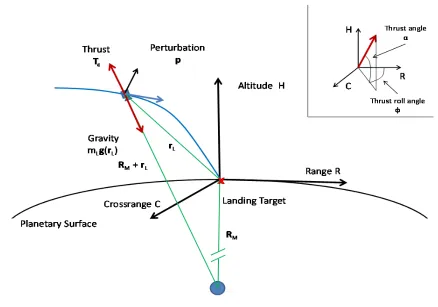
Figure 1 Guidance reference frame and free-body force diagram for a planetary lander during the powered descent to the designated target.

Potential functions methods are rooted in the Lyapunov stability theory for non-linear systems. Such methods are applied by defining a scalar potential function that may represent the topography of the landing location. To ensure the definition of a class of descent paths that globally converges to the selected target location, one must develop a class of guidance algorithms that ensure that the derivative of the potential function (gradient) along the trajectory is always negative. Following the standard Lyapunov definition of a potential function, and definingr as the current spacecraft position andrdthe desired position on the planets surface, we have

φ(rd) = 0

φ(r>0, ∀r6=rd

˙

φ(r<0, ∀r6=rd (10)

φ(r)→0, as ||r|| → ∞

According to the second Lyapunovs theorem, it can be shown that the desired pointrdis globally attractive and all trajectories converge toward it. On this basis, McInnes32used the potential function method to generate families of descent path toward the lunar surface as follows:

• The direction of the velocity vector, which in turn define the trajectory path, is shaped using a potential function containing geometric information about the terrain surrounding the landing location. As a result, one can find an acceleration command that forces the vehicle to follow the negative of the gradient potential, which ensure global convergence to the desired location.

For a given potential functionφ(r)that satisfies Eq.(10), one can define a velocity field as follows

v=−v(h) ∇φ(r)

||∇φ(r)||, (11) where v(h) is a pre-defined velocity-altitude profile (velocity magnitude shape). If the potential function has an analytical expression, one can easily find the acceleration command required to follow the prescribed path as defined by the potential function and the initial conditions. Indeed, the acceleration command is found as follows

ac = Λv−g (12)

˙

v = Λv, Λ=

∂v

∂r

3×3

, (13)

whereΛis the3×3matrix of partial derivatives of the velocity components andgis the gravity vector. Whereas this method has been previously studied, here we propose and evolution of the potential function-based methodology by a) numerically approximating the gradient of the potential function that yield a set of shaped path that are fuel-efficient and enforce specific trajectory con-straints and b) define a guidance algorithm that tracks the optimal velocity field as function of the position.

EXTREME LEARNING MACHINES

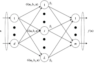
Computational intelligence techniques have been successfully used in learning functional rela-tionships that are only described by a limited about of data points. Most of such techniques (e.g. Neural Networks (NN), Support Vector Machines (SVM)) are faced with many challenges includ-ing, slow learning speed, poor computational scalability as well as requirement of ad-hoc human intervention. Extreme Learning Machines have been recently established as an emergent technol-ogy that may overcome some of the abovementioned challenges providing better generalization, faster learning speed and minimum human intervention. ELMs work with the ‘generalized‘ Single Layer Forward Networks (see Figure 2). SLFN are computationally designed to have a single hid-den layer (which can be either Radial Basis Function (RBF) or other activation functions) couple to a linear output layer. The key point is that the hidden neurons need not to be tuned and their weights (training parameters) can be sampled from a random distribution. Theoretical studies39show that feed-forward networks with minimum output weights tend to achieve better generalization. EML tend to reach a) the minimum training error and b) the smallest norm of output weights with conse-quent improved generalization. Importantly, since the hidden nodes can be selected and fixed, the output weights can be determined via least-square methodologies.

Figure 2 Typical architecture of a Single Layer Forward Network (SLFN) which is the most fundamental EML.

fL(x) = L X

i=1

β_igi(x) = L X

i=1

β_iG(ai, bi,x) (14)

withx∈_Rd_,β

i∈Rm.

For additive nodes with activation functiong

G(ai, bi,x) =g(aix+bi) (15)

withai∈Rm, bi∈R.

For RBF nodes with activation functiong

G(ai, bi,x) =g(bi||x−ai|| with ai ∈Rm, bi ∈R+. (16)

Consider a training set comprisingN distinct samples, [xi,ti] ∈ Rd×Rm.The mathematical model describing SLFNs can be cast as follows

L X

i=1

βiG(ai, bi,x) =tj, f or j∈1,· · ·, N. (17)

Compactly, we have

where the hidden layer output matrixH is formally written as

H=



 

h(x1) .. . h(xN)

  =   

G(a1, b1,x1) . . . G(aL, bL,xL) ..

.

G(a1, b1,xN) . . . G(aL, bL,xN) 

 

N×L

, with β=   

βT₁ .. . βT_L



 

L×m

,

T =



 

TT₁ .. . TT_N



 

N×m

.

Huang et al.36theoretically showed that SLFNs with randomly generated additive or RFB nodes can universally approximate any desired (target) function over a compact subset ofX ∈_Rd_{. Such} results can be generalized to any piecewise continuous activation function in the hidden node. The following theorem holds true:

Theorem 1 Given any non-constant piecewise continuous functiong:R→R, ifspan{G(a, b,x) :

(a, b) ∈ _Rd_×

R} is dense in L2, any continuous target function f and any function sequence {gL(x) = G(aL, bL,x)} randomly generated based on any continuous sampling distribution,

limL→∞||f −fL||holds with probability one if the output weightsβi are determined by ordinary

least square to minimize||f(x)−PL

i=1βigi(x)||.

The basic ELM can be constructed as follows. After selecting a sufficiently high number of hidden nodes (ELM architecture), the parameters(ai, bi)are randomly generated and remain fixed. Training occurs by simply finding a least-square solutionβof the systemHβ=T, i.e. findβˆsuch that

||Hβˆ −T||=minβ||Hβ−T||. (19)

FUEL-EFFICIENT VELOCITY FIELD COMPUTATION USING EXTREME LEARNING MACHINES

However, an explicit, closed-form representation of eitherφ(r,rd)and/orv(r,rd)is not generally available. However, if sufficient samples representing the functional relationship between poten-tial function and position, as well as velocity and position, are available, one can employ machine learning techniques to numerically approximate the desired function. Over the past two decades, Neural Networks (NN) have emerged as powerful computational devise capable of approximate any piecewise continuous function to the desired degrees. Biologically inspired, NNs are comprised of computational units called neurons that have the ability to learn the relationship between any desired function (assuming that certain conditions are satisfied) from inputs-output example. Here the goal is employ a class of neural networks called Extreme Learning Machines (ELM)35, 36to approximate the fuel-efficient velocity field.

NETWORK DESIGN AND TRAINING SET GENERATION USING PSEUDO-SPECTRAL METHODS

At the core of the proposed methodology is the ability to approximate a fuel-optimal velocity field that is representative of the gradient of a potential function. We employ ELM theory and we design and train a SLFN capable of approximating v(r,rd). The development goes through the following stages: 1) training set generation, 2) SLFN architecture design, 3) Training phase and 4) testing and validation phase.

The minimum-fuel problem for planetary landing can be defined as follows: Find the thrust program that minimizes the following cost function (negative of the lander final mass; equivalent to minimizing the amount of propellant during descent)

maxtF,T(.)mL(tF) =mintF,T(.) Z tF

0

||T||dt, (20)

subject to

¨

rL = −gL+ T

mL

, (21)

d

dtmL = −

||T||

Ispg0

, (22)

and the following boundary conditions

0< Tmin <||T||< Tmax (23)

rL(0) =rL0, vL(0) =r˙L(0) =vL0 (24) rL(tF) =rLF, vL(tF) =r˙L(tF) =vLF (25)

mL(0) =mLwet (26)

(a) (b)

Figure 3. (a) Samples of fuel-efficient trajectoties; (b) Samples of fuel-efficient velocity vectors.

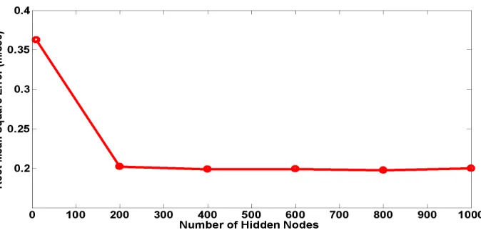
Figure 4. Root Mean Square Error (RMSE) as function of SLFN number of hidden nodes.

PARAMETER DESIGN

Samples from an optimal (continuous) vector field are generated by numerically computing a set of fuel-efficient trajectories via proper application of the optimal control theory. A set of 2−D

(vertical plane)38 fuel-optimal trajectories have been computed that are initiated at an altitude of

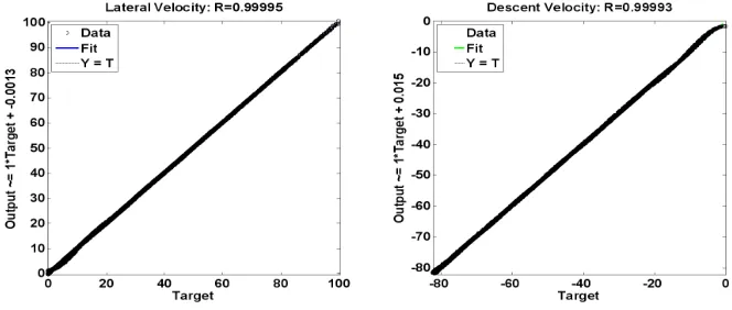
Figure 5 Test and validation regression plots: (a) Regression on lateral velocity; (b) Regression on descent velocity.

traning set is comprised ofN = 201×161 = 32361training samples. Figure 3 shows trajectories and velocity sampled from the training set.

ELM DESIGN: TRAINING AND TEST

The network is comprised of an input layer (three nodes describing the current position) and hid-den layer (number of nodes defined by the designer) and an output layer (three nodes that output the component of the optimal position). For a set ofLhidden nodes and the above specified training set, the following steps are taken to design the SLFN capable of approximating thevOP T =v(r,rd)

• randomly generate the parameters describing the hidden nodes(ai, bi) f or i= 1,· · · , L

• Compute the hidden layer output matrixH

• Compute the output weight vectorβby solvingH+β=T

The matrixH+=HT(HHT)−1H+orH+=(HTH)−1HT ifHHT is singular) is called the Moore-Penrose generalized inverse matrix. In computing the weights β, a positive value 1_λ was added to the diagonal ofHTH to improve the stability. Importantly, the linear weights and the ELM output function are computed as follows

β = HT

1

λ+HH

T

−1

T, (27)

vOP T(r,rd) = h(r)β=h(r)HT

1

λ+HH

T

−1

T. (28)

One critical aspect of the ELM implementation is the selection of the the hidden number of nodes which is a typical network design parameter. The matrix has dimensionN×LwhereN = 16180

systematically increasing the number of neurons and recording the training performances. Figure 4 shows the root square mean error as function of the number of hidden layers. As the number of hidden nodes is increased, the root mean square error stabilizes. A value ofL = 600 nodes has been selected as optimal architecture.

The SLFN design is tested and validated on a set of data comprising data points belonging to the training set on which the network has not been trained. Fifty percent of the overall training set is devoted to test and validation. Indeed, after proper training, the SLFN is run on test and validation input points and the output response predicted. A complete regression analysis is then illustrated in Figure 5. The later shows that the designed network has generalized well, i.e. has learned the vOP T =v(r,rd)functional relationship on points not included in the training set.

(a) (b)

(c) (d)

(a) (b)

(c)

Figure 7. 3-D Monte Carlo trajectories and landing ellipses.

EVALUATION OF GUIDANCE ALGORITHM PERFORMANCE

Two-Dimensional Results

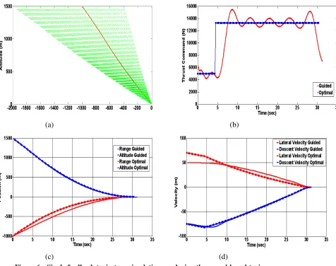
been compared with a newly generated numerical optimal solution generated via GPOPS that starts with the same initial conditions as the guided trajectory. Performance are comparable although it is worth noting that the neural-based trajectory shaping algorithm has not been designed to track the GPOPS-generated optimal fueld solution, but tracks the velocity field as approximated by the ELM. The open-loop, fuel efficient numerical solution achieve the desired target position with exactly zero velocity. The guided trajectory will generate guidance residual errors and it is not expect to have the same accuray of the open-loop ideal case. The magnitude of the thrust command oscillate as function of time as shown in Figure 6. This is due to the LQR design that has been chosen for the specific implementation. Importantly, in the last 10 seconds of the powered descent, the thrust command is reduced, which is probably the major cause of residual guidance errors. As noted it is not expected the guidance algorithm track exactly open-loop optimal trajectories. Indeed, as the lander moves across the vector field, the position associated to the guided trajectory trigger ELM outputs that approximate optimal velocity vectors associated to different fueld-optimal trajectories.

(a) (b)

(c)

Three-Dimensional Results

In this section, the neural-based trajectory shaping guidance performance is implemented and evaluated in a full3−Denvironment. is fairly straightforward. The2−DSLFN38has been used as reference and generate an axial-symmetric conical optimal vector field, by rotating the current

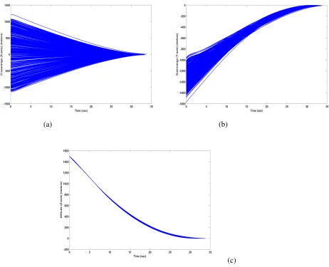
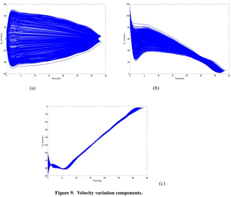
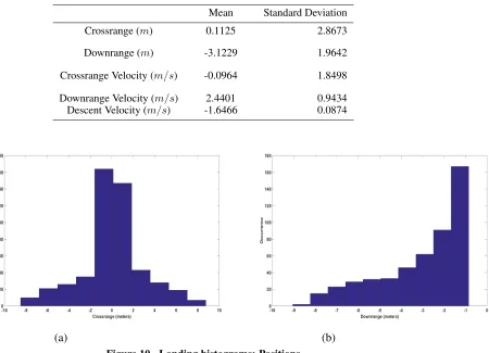
2−Dfield around the vertical(z−axis). To evaluate further the guidance algorithm performance, a set of 1000 Monte Carlo simulations have been implemented as shown in Figure 7. A set of randomly generated initial conditions have been generated by randomly perturbing the samples of initial conditions taken from the training set. Initial altitude and downrange are perturbed by a gaussian noise with zero mean and 10 meters standard deviation (1σ) (see Figure 8). Initial lateral and descent velocities are perturbed by a gaussian noise with zero mean and 2 m/sec standard deviation (1σ) as shown in Figure 9. Table 1 reports the landing statistics for the Monte Carlo Simulations. Figures 10, 11 show the landing histograms for the 1000 Monte Carlo simulations. The guidance algorithm is shown to perform well.

(a) (b)

(c)

Table 1. Landing Statistics for the Monte Carlo Simulations.

Mean Standard Deviation

Crossrange (m) 0.1125 2.8673

Downrange (m) -3.1229 1.9642

Crossrange Velocity (m/s) -0.0964 1.8498

Downrange Velocity (m/s) 2.4401 0.9434 Descent Velocity (m/s) -1.6466 0.0874

(a) (b)

(a) (b)

(c)

CONCLUSIONS

In this paper, the neural-based trajectory shaping guidance performance has been implemented and evaluated in a full3−Denvironment. The proposed efficient algorithm is also tested in typ-ical simulation scenarios which include a set of Monte Carlo simulation to evaluate the guidance performances. An approach to feedback guidance for planetary landing that may represent the next evolution of path shaping algorithms has also been illustrated. Conventional path shaping algo-rithms, as investigated for lunar descent and landing, have been based on the idea of defining a potential function that exhibits the typical properties of a Lyapunov function. In previous studies, potential functions have been selected to be analytical (e.g. quadratic function or any of its linear combination). Despite the convenience (e.g. vector field and acceleration command can be com-puted analytically), the families of trajectories generated in this fashion in generally non-optimal. The next evolution of trajectory shaping employs modern machine learning techniques to approxi-mate a potential function as function of position that generates trajectories that are attractive to the target and fuel efficient. Apparently, what is really needed is an algorithm that computes the optimal velocity field as function of the spacecraft actual position. Fuel efficient trajectories and velocities cannot be computed analytically, but numerical computation is required by using methods borrowed from optimal control theory (e.g. pseudo-spectral methods). ELM can be designed and trained on the output of open-loop, fuel-efficient trajectories generated via GPOPS. Such trajectories are shown to be convergent to the target and can be easily generated off-line. EML have shown to be fast and accurate in learning the desired functional relationship between the spacecraft position and the op-timal velocity field. For real-time implementation, the guidance algorithm evaluate current position and velocity, compute via ELM the actual desired velocity and employs a LQR to track the velocity field. Guidance simulations have demonstrated the ability of the guidance algorithm to drive the lander toward the desired position exhibiting low residual errors in both terminal downrange, lateral velocity and impact velocity.

REFERENCES

[1] R. D. Braun and R. M. Manning, “Mars Exploration Entry, Descent, and Landing Challenges,”Journal of Spacecraft and Rockets, Vol. 44, No. 2, March-April 2007, pp. 310–323.

[2] B. Steinfeldt, M. Grant, D. Matz, and R. Braun, “Guidance, Navigation, and Control Technology System Trades for Mars Pinpoint Landing,”Atmospheric Flight Mechanics Conference and Exhibit, Honolulu, HI, August 18-21 2008. Paper AIAA 2008-6216.

[3] A. A. Wolf, J. Tooley, S. Ploen, M. Ivanov, B. Acikmese, and K. Gromov, “Performance Trades for Mars Pinpoint Landing,”IEEE Aerospace Conference Proceedings, March 2006. Paper IEEE-1661. [4] A. A. Wolf, Sklyanskly, J. Tooley, and B. Rush, “Mars Pinpoint Landing Systems Trades,”In AIAA/AAS

Astrodynamics Specialist Conference, Mackinac Island, Michigan, August 19-23 2007. Paper AAS 07-310.

[5] K.-Y. Tu, M. S. Munir, K. D. Mease, and D. S. Bayard, “Drag-Based Predictive Tracking Guidance for Mars Precision Landing,”Journal of Guidance, Control and Dynamics, Vol. 23, No. 4, July-August 2000, pp. 620–628.

[6] U. Topcu, J. Casoliva, and K. D. Mease, “Fuel Efficient Powered Descent Guidance for Mars Landing,”

In AIAA Guidance, Navigation, and Control Conference and Exhibit, San Francisco, California, August 15 - 18, 2005. AIAA 2005-6286.

[7] R. R. Sostaric and J. R. Rea, “Powered Descent Guidance Methods for the Moon and Mars,”In AIAA Guidance, Navigation, and Control Conference and Exhibit, San Francisco, California, August 15 - 18, 2005. AIAA 2005-6287.

[8] F. Najson and K. D. Mease, “Computationally Inexpensive Guidance Algorithm for Fuel-Efficient Terminal Descent,” Journal of Guidance, Control and Dynamics, Vol. 29, No. 4, July-August 2006, pp. 955–964.

[10] G. Singh, A. M. SanMartin, and E. C. Wong, “Guidance and Control Design for Powered Descent and Landing on Mars,”In Aerospace Conference IEEE, Big Sky, Montana, March 3 - 10, 2007.

[11] A. R. Klumpp, “A Manually Retargeted Automatic Landing System for the Lunar Module (LM),” Jour-nal of Spacecraft and Rockets, Vol. 5, No. 2, February 1968, pp. 129–138.

[12] A. R. Klumpp, “Apollo Lunar Descent Guidance,”Automatica, Vol. 10, No. 2, March 1974, pp. 133– 146.

[13] J. Betts, “Survey of Numerical Methods for Trajectory Optimization,”Journal of Guidance, Control and Dynamics, Vol. 21, No. 2, March-April 1998, pp. 193–207.

[14] F. Fahroo and M. Ross, “Direct Trajectory Optimization by a Chebyshev Pseudospectral Method,” Jour-nal of Guidance, Control and Dynamics, Vol. 25, No. 1, January-February 2002, pp. 160–166.

[15] O. von Stryk and R. Bulirsch, “Direct and Indirect Methods for Trajectory Optimization,” Annals of Operations Research, Vol. 37, 1992, pp. 357–373.

[16] D. A. Benson, G. T. Huntington, T. P. Thorvaldsen, and A. V. Rao, “Direct Trajectory Optimization and Costate Estimation via an Orthogonal Collocation Method,” Journal of Guidance, Control and Dynamics, Vol. 29, No. 6, November-December 2006, pp. 1435–1440.

[17] A. V. Rao, D. A. Benson, C. Darby, M. A. Patterson, C. Francolin, and e. a. I. Sanders, “Algorithm 902: GPOPS, a MATLAB Software for solving Multiple Phase Optimal Control Problems using the Gauss Pseudospectral Method,”ACM Transactions on Mathematical Software, Vol. 37, No. 2, 2010, pp. 22:1–22:39.

[18] D. G. Hull, “Conversion of Optimal Control Problems into Parameter Optimization Problems,”Journal of Guidance, Control and Dynamics, Vol. 20, No. 1, January-February 1997, pp. 57–60.

[19] D. Kraft, “On Converting Optimal Control Problems into Nonlinear Programming Problems,”In Com-putational Mathematical ProgrammingF15of NATO ASI Series,K. Schittkowsky Ed., Springer, 1985, pp. 261–280.

[20] J. Vlassenbroeck and R. V. Dooren, “A Chebyshev Technique for Solving Nonlinear Optimal Control Problems,”IEEE Transactions on Automatic Control, Vol. 33, No. 4, April 1988, pp. 333–340. [21] O. von Stryk, “Numerical Solution of Optimal Control Problems by Direct Collocation,” In

Opti-mal Control - Calculus of Variation - OptiOpti-mal Control Theory and Numerical Methods,R. Bulirsch, A. Miele, J. Stoer and K. H. Well Eds., International Series of Numerical Mathematics, Vol. 111, Birkh¨auser, 1993, pp. 129–143.

[22] E. D. Dickmanns and K. H. Well, “Approximate Solution of Optimal Control Problems using Third Order Hermite Polynomial Functions,”Lecture Notes in Computer Science, Vol. 27, 1975, pp. 158– 166.

[23] P. J. Enright and B. A. Conway, “Discrete Approximations to Optimal Trajectories using Direct Tran-scription and Nonlinear Programming,”Journal of Guidance, Control and Dynamics, Vol. 15, No. 4, July-August 1992, pp. 994–1002.

[24] C. R. Hargraves and S. W. Paris, “Direct Trajectory Optimization using Nonlinear Programming and Collocation,”Journal of Guidance, Control and Dynamics, Vol. 10, No. 4, 1987, pp. 338–342.

[25] B. Ac¸ikmes¸e and S. R. Ploen, “Convex Programming Approach to Powered Descent Guidance for Mars Landing,”Journal of Guidance, Control and Dynamics, Vol. 30, No. 5, September-October 2007, pp. 1353–1366.

[26] J. F. Sturm, “Using SeDuMi 1.02, a MATLAB Toolbox for Optimization over Symmetric Cones,” Op-timization Methods and Software, Vol. 11, No. 1, 1999, pp. 625–653.

[27] J. F. Sturm, “Implementation of Interior Point Methods for Mixed Semidefinite and Second Order Cone Optimization Problems,”Optimization Methods and Software, Vol. 17, No. 6, 2002, pp. 1105–1154. [28] B. Ac¸ikmes¸e and L. Blackmore, “Lossless Convexification of a Class of Optimal Control Problems with

Non-Convex Control Constraints,”Automatica, Vol. 47, No. 2, February 2011, pp. 341–347.

[29] Y. Nesterov and A. Nemirovsky, “Interior-Point Polynomial Methods in Convex Programming,”SIAM, Philadelphia, PA, 1994.

[30] P. E. Gill, W. Murray, and M. A. Saunders, “SNOPT: An SQP Algorithm for Large Scale Constrained Optimization,”Technical Report NA 96-2, University of California, San Diego, CA, USA, 1996. [31] L. Blackmore, B. Ac¸ikmes¸e, and D. P. Scharf, “Minimum-Landing-Error Powered-Descent Guidance

for Mars Landing using Convex Optimization,”Journal of Guidance, Control and Dynamics, Vol. 33, No. 4, July-August 2010, pp. 1161–1171.

[32] C. R. McInnes, “Path Shaping Guidance for Terminal Lunar Descent,”Acta Astronautica, Vol. 36, No. 7, 1995, pp. 366–377.

[34] H. Guang-Bin, D. H. Wang, and Y. Lan, “Extreme Learning Machines: A Survey,”International Journal of Machine Learning and Cybernetics, Vol. 2, 2011, pp. 107–122.

[35] H. Guang-Bin, Q.-Y. Zhu, and C.-K. Siew, “Extreme Learning Machines: Theory and Applications,”

Neurocomputing, Vol. 70, 2006, pp. 489–501.

[36] H. Guang-Bin, L. Chen, and C.-K. Siew, “Universal Approximation using Incremental Constructive Feedforward Networks with Random Hidden Nodes,”IEEE Transactions on Neural Networks, Vol. 17, No. 4, July 2006, pp. 879–892.

[37] H. Guang-Bin and Z. Qin-Yu, “Real-Time Learning Capability of Neural Networks,”IEEE Transactions on Neural Networks, Vol. 17, No. 4, July 2006, pp. 863–878.

[38] R. Furfaro, J. Simo, B. Gaudet, and D. R. Wibben, “Neural-based Trajectory Shaping Approach for Ter-minal Planetary Pinpoint Guidance,”In AAS/AIAA Astrodynamics Specialist Conference, Hilton Head, South Carolina, August 11 - 15, 2013. AAS 13-875.