Franz, Sebastian and Kopteva, Natalia (2012) Greenʼs function estimates
for a singularly perturbed convection–diffusion problem. Journal of
Differential Equations, 252 (2). pp. 1521-1545. ISSN 0022-0396 ,
http://dx.doi.org/10.1016/j.jde.2011.07.033
This version is available at https://strathprints.strath.ac.uk/44835/
Strathprints is designed to allow users to access the research output of the University of Strathclyde. Unless otherwise explicitly stated on the manuscript, Copyright © and Moral Rights for the papers on this site are retained by the individual authors and/or other copyright owners. Please check the manuscript for details of any other licences that may have been applied. You may not engage in further distribution of the material for any profitmaking activities or any commercial gain. You may freely distribute both the url (https://strathprints.strath.ac.uk/) and the content of this paper for research or private study, educational, or not-for-profit purposes without prior permission or charge.
Any correspondence concerning this service should be sent to the Strathprints administrator:
Green’s function estimates for a singularly perturbed
convection-diffusion problem
∗
Sebastian Franz
†Natalia Kopteva
‡Abstract
We consider a singularly perturbed convection-diffusion problem posed in the unit square with a horizontal convective direction. Its solutions exhibit parabolic and exponential boundary layers. Sharp estimates of the Green’s function and its first- and second-order derivatives are derived in the L1 norm. The dependence of
these estimates on the small diffusion parameter is shown explicitly. The obtained estimates will be used in a forthcoming numerical analysis of the considered problem.
AMS subject classification (2000): 35J08, 35J25, 65N15
Key words: Green’s function, singular perturbations, convection-diffusion
1
Introduction
In this paper we investigate the Green’s function for the following problem posed in the unit-square domain Ω = (0,1)2:
Lxyu(x, y) :=−ε(uxx+uyy)−(a(x, y)u)x+b(x, y)u=f(x, y) for (x, y)∈Ω, (1.1a)
u(x, y) = 0 for (x, y)∈∂Ω. (1.1b)
Hereεis a small positive parameter, while the coefficients a andb are sufficiently smooth (e.g., a, b∈C∞( ¯Ω)). We also assume, for some positive constant α, that
a(x, y)≥α >0, b(x, y)−ax(x, y)≥0 for all (x, y)∈Ω¯. (1.2)
Under these assumptions, (1.1a) is a singularly perturbed elliptic equation, frequently referred to as a convection-dominated convection-diffusion equation. This equation serves as a model for Navier-Stokes equations at large Reynolds numbers or (in the linearised case) of Oseen equations and provides an excellent paradigm for numerical techniques in the computational fluid dynamics [19].
∗This work has been supported by Science Foundation Ireland under the Research Frontiers
Pro-gramme 2008; Grant 08/RFP/MTH1536
†Institut f¨ur Numerische Mathematik, Technische Universit¨at Dresden, 01062 Dresden, Germany
e-mail: [email protected]
‡Department of Mathematics and Statistics, University of Limerick, Limerick, Ireland
The asymptotic analysis for problems of type (1.1) is very intricate and illustrates the complexity of their solutions [11, Section IV.1], [12]. We also refer the reader to [20, Chapter IV], [19, Chapter III.1] and [13, 14] for pointwise estimates of solution derivatives. In short, solutions of problem (1.1) typically exhibit parabolic boundary layers along the characteristic boundaries y= 0 and y = 1, and an exponential boundary layer along the outflow boundaryx= 0. Furthermore, if a discontinuous Dirichlet boundary condition is imposed at the inflow boundary x = 1, then solutions also exhibit characteristic interior layers. Note that because of the complexity of the solutions, the analysis techniques [13, 14] work only for a constant-coefficient version of (1.1a). Note also that the complex solution structure is reflected in the corresponding Green’s function, which is the subject of this paper.
Our interest in considering the Green’s function of problem (1.1) and estimating its derivatives is motivated by the numerical analysis of this computationally challenging problem. More specifically, we shall use the obtained estimates in the forthcoming paper [7] to derive robust a posteriori error bounds for computed solutions of this problem using finite-difference methods. (This approach is related to recent articles [15, 4], which address the numerical solution of singularly perturbed equations of reaction-diffusion type.) In a more general numerical-analysis context, we note that sharp estimates for continuous Green’s functions (or their generalised versions) frequently play a crucial role in a priori and a posteriori error analyses [6, 10, 18].
We shall estimate the derivatives of the Green’s function in the L1 norm (as they will
be used to estimate the error in the computed solution in the dual L∞ norm [7]). Our
estimates will be uniform in the small perturbation parameter ε in the sense that any dependence on ε will be shown explicitly. Note also that our estimates will be sharp (in the sense of Theorem 2.6) up to an ε-independent constant multiplier.
As any Green’s function estimate implies a certain a priori estimate for the original problem, we also refer the reader to D¨orfler [5], who, for a similar problem, gives extensive a priori solution estimates that involve the right-hand side in various positive norms such as Lp and Wm,p with m≥ 0. In comparison, a priori solution estimates that follow from our results, involve negative norms of the right-hand side (see Corollary 2.3 and also Remark 2.4), so they are different in nature.
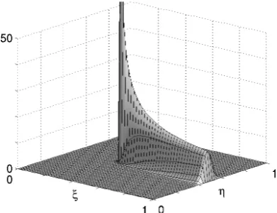
Our analysis in this paper resembles those in [15, Section 3], [4, Section 3] in that, roughly speaking, we freeze the coefficients and estimate the corresponding explicit Green’s function for a constant-coefficient equation, and then we investigate the difference between the original and the frozen-coefficient Green’s functions. This procedure is often called the parametrix method. The two cited papers deal with equations of reaction-diffusion type, for which the Green’s function in the unbounded domain is (almost) radially symmetric and exponentially decaying away from the singular point. By contrast, the Green’s func-tion for the convecfunc-tion-diffusion problem (1.1) exhibits a much more complexanisotropic structure (see Fig. 1). This is reflected in a much more intricate analysis compared to [15, 4], in particular, for the variable-coefficient case.
Figure 1: Typical anisotropic behaviour of the Green’s function for problem (1.1): a= 1,
b= 0, (x, y) = (1 3,
1
2) and ε = 10
−3.
Theorem 2.6. In Section 3, we obtain the fundamental solution for a constant-coefficient version of (1.1a) in the domain Ω =R2; this fundamental solution is bounded in Section 4. Next, in Section 5, using the method of images with an inclusion of cut-off functions, we define and estimate certain approximations of the constant-coefficient Green’s functions in the domains Ω = (0,1)×Rand Ω = (0,1)2. The difference between the frozen-coefficient
approximations of Section 5 and the original variable-coefficient Green’s function is esti-mated in Section 6; this completes the proof of Theorem 2.2. In the final Section 7 we discuss generalisation of our results to more than two dimensions.
Notation. Throughout the paper, C denotes a generic positive constant that may take different values in different formulas, but isindependent of the singular perturbation parameter ε. A subscripted C (e.g., C1) denotes a positive constant that takes a fixed
value, and is also independent of ε. Notation such as v = O(w) means |v| ≤ Cw for some C. The standard Sobolev spaces Wm,p(Ω′) and L
p(Ω′) on any measurable subset Ω′ ⊂ R2 are used for p ≥ 1 and m = 1,2. The L
p(Ω′) norm is denoted by k·kp;Ω′ while
the Wm,p(Ω′) norm is denoted by k·k
m,p;Ω′. Sometimes the domain of interest will be an
open ball B(x′, y′;ρ) := {(x, y) ∈ R2 : (x−x′)2 + (y−y′)2 < ρ2} centred at (x′, y′) of
2
Definition of the Green’s function. Main result
Let G = G(x, y;ξ, η) be the Green’s function associated with problem (1.1). For each fixed (x, y)∈Ω, it satisfies
L∗
ξηG(x, y;ξ, η) = −ε(Gξξ+Gηη) +a(ξ, η)Gξ+b(ξ, η)G=δ(x−ξ)δ(y−η), (ξ, η)∈Ω,
G(x, y;ξ, η) = 0, (ξ, η)∈∂Ω.
(2.1) HereL∗
ξη is the adjoint differential operator toLxy, whileδ(·) is the one-dimensional Dirac
δ-distribution, so the product δ(x−ξ)δ(y−η) is equivalent to the two-dimensional δ -distribution centred at (ξ, η) = (x, y); see [9, Example 3.29], [21, Section 5.5]. The unique solutionu of (1.1) has the representation
u(x, y) =
Z Z
Ω
G(x, y;ξ, η)f(ξ, η)dξ dη, (2.2)
(provided that f is sufficiently regular so that (2.2) is well-defined). Note that, for each fixed (ξ, η)∈Ω, the Green’s function Galso satisfies
LxyG(x, y;ξ, η) = −ε(Gxx+Gyy)−(a(x, y)G)x+b(x, y)G=δ(x−ξ)δ(y−η),(x, y)∈Ω,
G(x, y;ξ, η) = 0, (x, y)∈∂Ω.
(2.3) Therefore, the unique solution v of the adjoint problem
L∗xyv(x, y) = −ε(vxx+vyy) +a(x, y)vx+b(x, y)v =f(x, y) for (x, y)∈Ω,
v(x, y) = 0 for (x, y)∈∂Ω.
is given by
v(ξ, η) =
Z Z
Ω
G(x, y;ξ, η)f(x, y)dx dy. (2.4)
We first give a preliminary result for G.
Lemma 2.1. Under assumptions (1.2), the Green’s function G associated with problem (1.1) satisfies
Z 1
0 |
G(x, y;ξ, η)|dη≤C, kG(x, y;·)k1 ;Ω ≤C for (x, y)∈Ω, (2.5)
where C is some positive ε-independent constant.
Proof. The first estimate of (2.5) is given in the proof of [5, Theorem 2.10] (see also [19, Theorem III.1.22] and [3] for similar results). The second desired estimate follows.
Theorem 2.2. Let ε∈(0,1]. The Green’s function G associated with (1.1),(1.2) on the unit square Ω = (0,1)2 satisfies, for all (x, y)∈Ω, the following bounds
k∂ξG(x, y;·)k1 ;Ω ≤C(1 +|lnε|), (2.6a)
k∂ηG(x, y;·)k1 ;Ω+k∂yG(x, y;·)k1 ;Ω ≤Cε−1/2. (2.6b)
Furthermore, for any ball B(x′, y′;ρ) of radius ρ centred at any (x′, y′)∈Ω¯, we have
kG(x, y;·)k1,1 ;B(x′,y′;ρ)≤Cε−1ρ, (2.6c)
while for the ball B(x, y;ρ) of radius ρ centred at (x, y) we have
k∂ξ2G(x, y;·)k1 ;Ω\B(x,y;ρ) ≤Cε−1ln(2 +ε/ρ), (2.6d)
k∂η2G(x, y;·)k1 ;Ω\B(x,y;ρ) ≤Cε−1(ln(2 +ε/ρ) +|lnε|). (2.6e)
Here C is some positive ε-independent constant.
The rest of the paper is devoted to the proof of this theorem, which is completed in Section 6.
In view of the solution representation (2.2), the bounds (2.6a), (2.6b) immediately imply the following a priori solution estimates for our original problem.
Corollary 2.3. Let f(x, y) = ∂xF1(x, y) +∂yF2(x, y) with F1, F2 ∈ L∞(Ω). Then there
exists a unique solution u∈L∞(Ω) of problem (1.1), (1.2), for which we have the bound
kuk∞;Ω ≤C
(1 +|lnε|)kF1k∞;Ω+ε−1/2kF2k∞;Ω
. (2.7)
Proof. Represent u using (2.2). Then integrate by parts and use (2.6a) and (2.6b).
Remark 2.4. Let us associate the components∂xF1 and∂yF2 off with the one-dimensional
parts −ε∂2
x −∂xa(x, y) and −ε∂y2+b(x, y), respectively, of the operator Lxy. Then, bar the weak logarithmic factor |lnε|, the bound (2.7) clearly resembles the corresponding one-dimensional a priori solution estimates. Indeed, for the one-dimensional equations −εu′′
1(x)− (a1(x)u1(x))′ = f1(x) and −εu′′2(x) + b2(x)u2(x) = f2(x) (where a1, b2 ≥
C > 0) subject to u1,2(0) = u1,2(1) = 0, one has ku1k∞;(0,1) ≤ Ckf1k−1,∞;(0,1), and
ku2k∞;(0,1) ≤Cε−1/2kf2k−1,∞;(0,1), wherek · k−1,∞;(0,1) is the norm in the negative Sobolev
space W−1,∞(0,1) (see, e.g., [17, Theorem 3.25]).
Remark 2.5. In the proof of Corollary 2.3, the existence of a solutionu∈L∞(Ω)of
prob-lem (1.1),(1.2)follows from the observation that the solution representation formula (2.2) yields a bounded function. Note that the existence of a bounded solution of this problem, under the additional mild assumption b(x, y)− 12∂xa(x, y) ≥ 0, can be shown by an ap-plication of [16, Chapter 3, Theorems 5.2 and 13.1]. In particular, the second cited theorem states that if there exists a solution u ∈ W2,1(Ω), then it is bounded in Ω¯ by
Note that the upper estimates of Theorem 2.2 are sharp in the following sense. Theorem 2.6([8]). Letε∈(0, c0] for some sufficiently small positivec0. Set a(x, y) :=α
and b(x, y) := 0 in (1.1). Then the Green’s function G associated with this problem on the unit square Ω = (0,1)2 satisfies, for all (x, y)∈[1
4, 3 4]
2, the following lower bounds:
k∂ξG(x, y;·)k1;Ω ≥c|lnε|, (2.8a)
k∂ηG(x, y;·)k1;Ω ≥c ε−1/2. (2.8b)
Furthermore, for any ball B(x, y;ρ) of radius ρ≤ 18, we have
kG(x, y;·)k1,1;Ω∩B(x,y;ρ) ≥
(
c ρ/ε, if ρ≤2ε,
c(ρ/ε)1/2, otherwise, (2.8c)
k∂ξ2G(x, y;·)k1;Ω\B(x,y;ρ) ≥c ε−1ln(2 +ε/ρ), if ρ≤c1ε, (2.8d)
k∂η2G(x, y;·)k1;Ω\B(x,y;ρ) ≥c ε−1(ln(2 +ε/ρ) +|lnε|), if ρ≤ 18. (2.8e)
Here c and c1 are ε-independent positive constants.
This result can be anticipated from an inspection of the bounds for an explicit funda-mental solution in a constant-coefficient case; see Section 4.
3
Fundamental solution in a constant-coefficient case
In this section we shall explicitly solve simplifications of the two problems (2.1) and (2.3) that we have for G. To get these simplifications, we employ the parametrix method and so freeze the coefficients in these problems by replacing a(ξ, η) by a(x, y) in (2.1), and replacing a(x, y) bya(ξ, η) in (2.3), and also setting b:= 0; the frozen-coefficient versions of the operators L∗
ξη and Lxy will be denoted by ¯L∗ξη and ˜Lxy, respectively. Furthermore, we extend the resulting equations to R2 and denote their solutions by ¯g and ˜g. Thus we get
¯
L∗ξη¯g(x, y;ξ, η) =−ε(¯gξξ+ ¯gηη) +a(x, y) ¯gξ =δ(x−ξ)δ(y−η) for (ξ, η)∈R2, (3.1) ˜
Lxyg˜(x, y;ξ, η) =−ε(˜gxx+ ˜gyy)−a(ξ, η) ˜gx =δ(x−ξ)δ(y−η) for (x, y)∈R2. (3.2)
As the variables (x, y) appear as parameters in equation (3.1) and (ξ, η) appear as pa-rameters in equation (3.2), we effectively have two equations with constant coefficients. A calculation (see Remark 3.1 below for details) yields explicit representations of their solutions by
¯
g(x, y;ξ, η) =g(x, y;ξ, η;q)
q=1 2a(x,y)
, ˜g(x, y;ξ, η) = g(x, y;ξ, η;q)
q=1 2a(ξ,η)
. (3.3)
Here the function g is defined, using the modified Bessel function of the second kind of order zero K0(·), by
g =g(x, y;ξ, η;q) := 1 2πεe
qξˆ[x]K
0(qrˆ[x]), (3.4a)
ˆ
ξ[x]:= (ξ−x)/ε, ηˆ:= (η−y)/ε, ˆr[x] :=
q
ˆ
ξ2
We use a subindex in ˆξ[x] and ˆr[x] to highlight their dependence on x as in many places
x will take different values; but when there is no ambiguity, we shall sometimes simply write ˆξ and ˆr.
Remark 3.1. The representation (3.4) is given in [19, (III.1.16)]. For completeness, we sketch a proof of (3.3),(3.4) for g¯. Set q = 12a(x, y) and g¯=V(ξ, η)eqξ/ε in (3.1). Now a calculation shows that
−ε2(Vξξ+Vηη) +q2V =ε e−qξ/εδ(x−ξ)δ(y−η).
Here in the right-hand side, one has e−qξ/εδ(x−ξ) =e−qx/εδ(x−ξ). As the fundamental solution for the operator −ε2(∂2
ξ +∂η2) +q2 is 2πε12K0(qr/ε) [22, Chapter VII], so V =
ε e−qx/ε 1
2πε2K0(qr/ε), and the desired representation (3.3),(3.4)for¯g immediately follows.
Remark 3.2. Note that the solution g¯ of (3.1) is not the fundamental solution for the operator L¯∗
ξη. Indeed, denoting the latter by Γ = Γ(x, y;ξ, η;s, t), one has the equation ¯
L∗
ξηΓ =δ(s−ξ)δ(t−η), in which (x, y)appear as parameters. So imitating the calculation in Remark 3.1, one gets Γ(x, y;ξ, η;s, t) = g(s, t;ξ, η;q)
q=12a(x,y) (compare with (3.3)).
Similarly, the solution g˜of (3.2) is not the fundamental solution for the operator L˜xy.
The function g and its derivatives involve the modified Bessel functions of the second kind of order zeroK0(·) and of order oneK1(·). With the notationK0,1 := max{K0, K1},
we quote some useful properties of the modified Bessel functions [1]:
K0,1(s)≤Cs−1e−s/2 ∀s >0, K0,1(s)≤Cs−1/2e−s ∀s≥C >0, (3.5a)
K0(z) =K1(z)
1− 1
2z +O(z
−2)
. (3.5b)
4
Bounds for the fundamental solution
g
(
x, y
;
ξ, η
;
q
)
Throughout this section we assume that Ω = (0,1)×R, but all results remain valid for Ω = (0,1)2. Here we derive a number of useful bounds for the fundamental solution g
of (3.4) and its derivatives that will be used in Section 5. As sometimes q = 1
2a(x, y) or
q= 12a(ξ, η) (as in (3.3)), we shall also use the full-derivative notation
Dη :=∂η +12∂ηa(ξ, η)·∂q, Dy :=∂y +12∂ya(x, y)·∂q. (4.1)
Lemma 4.1. Let (x, y) ∈ [−1,1]×R and 0 < 12α ≤ q ≤ C. Then for the function
g =g(x, y;ξ, η;q) of (3.4) we have the following bounds
kg(x, y;·;q)k1 ;Ω ≤C, (4.2a)
k∂ξg(x, y;·;q)k1 ;Ω ≤C(1 +|lnε|), (4.2b)
ε1/2k∂ηg(x, y;·;q)k1 ;Ω+k∂qg(x, y;·;q)k1 ;Ω ≤C, (4.2c)
k(εrˆ[x]∂ξg)(x, y;·;q)k1 ;Ω ≤C, (4.2d)
and for any ball B(x′, y′;ρ) of radius ρ centred at any (x′, y′)∈[0,1]×R, we have
kg(x, y;·;q)k1,1 ;B(x′,y′;ρ) ≤Cε−1ρ, (4.2f)
while for the ball B(x, y;ρ) of radius ρ centred at (x, y), we have
k∂ξ2g(x, y;·;q)k1 ;Ω\B(x,y;ρ) ≤Cε−1ln(2 +ε/ρ), (4.2g)
k∂η2g(x, y;·;q)k1 ;Ω\B(x,y;ρ) ≤Cε−1(ln(2 +ε/ρ) +|lnε|). (4.2h)
Furthermore, one has the bound
k∂xg(x, y;·;q)k1 ;Ω ≤C(1 +|lnε|), (4.3a)
and, with the full-derivative notation (4.1), the bounds
kDηg(x, y;·;q)k1 ;Ω+kDyg(x, y;·;q)k1 ;Ω ≤Cε−1/2, (4.3b)
k(εrˆ[x]Dη∂xg)(x, y;·;q)k1 ;Ω+k(εrˆ[x]Dy∂ξg)(x, y;·;q)k1 ;Ω ≤Cε−1/2. (4.3c)
Proof. First, note that ∂xg = −∂ξg and ∂yg = −∂ηg, so (4.3a) follows from (4.2b), (4.3b) follows from (4.1), (4.2c), while (4.3c) follows from (4.1), (4.2e). Thus it suffices to establish the bounds (4.2).
Throughout the proof, x and y are fixed so we employ the notation ˆξ := ˆξ[x] and
ˆ
r:= ˆr[x]. A calculation shows that the first-order derivatives ofg(x, y;ξ, η;q) are given by
∂ξg = 2πεq2 eq
ˆ
ξhK
0(qˆr)−
ˆ
ξ
ˆ
rK1(qrˆ)
i
, (4.4a)
∂ηg =−2πεq2 e
qξˆhηˆ ˆ
rK1(qrˆ)
i
, (4.4b)
∂qg = 2πε1 reˆ q
ˆ
ξhξˆ ˆ
rK0(qrˆ)−K1(qrˆ)
i
. (4.4c)
Here we usedK′
0 =−K1, [1], and then ∂ξrˆ=ε−1ξ/ˆ rˆand∂ηrˆ=ε−1η/ˆ rˆ. In a similar man-ner, but additionally using K′
1(s) = −K0(s)−K1(s)/s [1], and also∂ξ(ˆη/rˆ) =−ε−1ξˆη/ˆ rˆ3 and ∂η(ˆη/rˆ) = ε−1ξˆ2/rˆ3, one gets the second-order derivatives
∂ξη2 g = 2πεq3 e
qξˆ ηˆ ˆ
r2
h
qrˆξˆ ˆ
rK0(qrˆ)−K1(qrˆ)
+ 2ξˆ ˆ
rK1(qrˆ)
i
, (4.5a)
∂ξq2 g = 2πεq2 eq
ˆ
ξrˆ−1hξˆˆr
{2K0(qrˆ) + q1ˆrK1(qrˆ)} −( ˆξ2 + ˆr2)K1(qrˆ)
i
+q−1∂ξg, (4.5b)
∂η2g = 2πεq3 eq
ˆ
ξhqηˆ2 ˆ
r2K0(qrˆ) +
ˆ
η2−ξˆ2
ˆ
r3 K1(qrˆ)
i
. (4.5c)
Finally, combining ∂2
ξg =−∂ξ2g+
2q
ε ∂ξg with (4.4a) and (4.5c) yields
∂ξ2g = 2πεq3 eq
ˆ
ξhqK
0(qrˆ) +
ˆ
ξ2
ˆ
r2K0(qˆr)−2
ˆ
ξ
ˆ
rK1(qrˆ)
+ξˆ
2−ηˆ2
ˆ
r3 K1(qrˆ)
i
Now we proceed to estimating the above derivatives of g. Note that dξ dη =ε2dξ dˆ ηˆ,
where ( ˆξ,ηˆ)∈Ω :=ˆ ε−1(−x,1−x)×
R⊂(−∞,2/ε)×R. Consider the domains
ˆ Ω1 :=
ˆ
ξ <1 + 14|ηˆ| , Ωˆ2 :=
max{1,14|ηˆ|}<ξ <ˆ 2/ε .
As ˆΩ ⊂Ωˆ1∪Ωˆ2 for any x ∈[−1,1], it is convenient to consider integrals over these two
subdomains separately.
(i) Consider ( ˆξ,ηˆ)∈Ωˆ1. Then ˆξ ≤1 +14rˆso, with the notationK0,1 := max{K0, K1},
one gets
ε2
(1 + ˆr)(ε−1|g|+|∂ξg|+|∂ηg|+|∂qg|+|∂ξq2 g|) +εrˆ|∂ξη2 g|
≤Ceqξˆ(1 + ˆr+ ˆr2)K0,1(qˆr)
≤Crˆ−1e−qr/ˆ 8, (4.6)
where we combined eqξˆ≤eq(1+ˆr/4) with 1 + ˆr+ ˆr2 ≤ Ceqˆr/8 (which follows from q ≥ 1 2α)
and K0,1(qrˆ)≤C(qˆr)−1e−qˆr/2 (see (3.5a)). This immediately yields
Z Z
ˆ Ω1
(1 + ˆr)(ε−1|g|+|∂ξg|+|∂ηg|+|∂qg|+|∂ξq2 g|) +εrˆ|∂ξη2 g|
ε2dξ dˆ ηˆ
≤C
Z ∞
0
e−qˆr/8drˆ
≤C. (4.7)
Similarly,
ε2
|∂ξ2g|+|∂η2g|
≤Cε−1eqξˆ(1 + ˆr−1)K0,1(qˆr)≤Cε−1rˆ−2e−qr/ˆ 8,
so
Z Z
ˆ
Ω1\B(0,0;ˆρ)
|∂2
ξg|+|∂η2g|
ε2dξ dˆ ηˆ
≤Cε−1
Z ∞
ˆ
ρ ˆ
r−1e−qr/ˆ 8drˆ≤Cε−1ln(2 + ˆρ−1). (4.8)
Furthermore, for an arbitrary ball ˆBρˆ of radius ˆρ in the coordinates ( ˆξ,ηˆ), we get
Z Z
ˆ Ω1∩Bˆρˆ
|∂ξg|+|∂ηg|+|g|
ε2dξ dˆ ηˆ
≤C
Z ρˆ
0
e−qr/ˆ 8drˆ≤Cmin{ρ,ˆ 1}. (4.9)
(ii) Next consider ( ˆξ,ηˆ) ∈ Ωˆ2. In this subdomain, it is convenient to rewrite the
integrals in terms of ( ˆξ, t), where
t := ˆξ−1/2ηˆ so ξˆ−1/2dηˆ=dt, rˆ−ξˆ= ηˆ
2
ˆ
r+ ˆξ ≤t
2. (4.10)
Note that qrˆ≥q ≥ 12αin ˆΩ2, soK0,1(qˆr)≤C(qrˆ)−1/2e−qˆr by the second bound in (3.5a).
We also note that ˆξ ≤ rˆ ≤ √17 ˆξ in ˆΩ2 so ˆr−ξˆ= ˆη2/(ˆr+ ˆξ) ≥ c0ηˆ2/ξˆ= c0t2, where
c0 := (1 +
√
17)−1. Consequentlye−q(ˆr−ξˆ) ≤e−qc0t2, so
eqξˆK0,1(qrˆ)≤CQ for ( ˆξ,ηˆ)∈Ωˆ2, where Q:= ˆξ−1/2e−qc0t
2
and
Z
R
(1 +|t|+t2+|t|3+t4)Q dηˆ≤C
Z
R
(1 +|t|+t2+|t|3+t4)e−qc0t2dt ≤C. (4.12)
We now claim that for g and its derivatives in ˆΩ2 one has
ε2|g| ≤C ε Q, (4.13a)
ε2|∂ηg| ≤Cξ−1/2|t|Q, (4.13b)
ε2|∂η2g| ≤C ε−1ξˆ−1[t2+ 1]Q. (4.13c)
Here (4.13a) is straightforward, and (4.13b) immediately follows from (4.4b) as |ηˆ|/ˆr ≤ |ηˆ|/ξˆ=ξ−1/2|t|. The next bound (4.13c) is obtained from (4.5c) using ˆη2/rˆ2 ≤ξ−1t2 and
|ηˆ2−ξˆ2|/ˆr3 ≤rˆ−1 ≤ξˆ−1.
Furthermore, we claim that in ˆΩ2 one also has
ε2(εrˆ|∂ξg|+|∂qg|) ≤ C ε[t2+ 1]Q, (4.13d)
ε2|∂ξg| ≤ Cξˆ−1[t2+ 1]Q, (4.13e)
ε2(εrˆ|∂ξη2 g|) ≤ Cξˆ−1/2|t|[t2+ 1]Q, (4.13f)
ε2(εrˆ|∂ξq2 g|) ≤ C ε[t4+ 1]Q+q−1ε2(εrˆ|∂ξg|), (4.13g)
ε2|∂ξ2g| ≤ C ε−1ξˆ−2[t4+ 1]Q. (4.13h)
To get (4.13d), we combine (4.4a) and (4.4c) with the observation that
|Kν(qrˆ)− ˆ
ξ
ˆ
rKµ(qrˆ)|=
1−
ˆ
ξ
ˆ
r +O(ˆr
−1)
K1(qˆr) for ˆr ≥1, (4.14a)
≤Crˆ−1[t2+ 1]K1(qrˆ) for ˆξ ≥1, (4.14b)
where ν, µ = 0,1. Note that (4.14a) and (4.14b) are easily verified using (3.5b) and ˆ
r−ξˆ≤ t2 from (4.10), respectively. The bound (4.13e) follows from the bound for ∂
ξg in (4.13d) as ˆr−1 ≤ξˆ−1. We now proceed to (4.13f), which is obtained from (4.5a) again
using |ηˆ|/ˆr ≤ ξ−1/2|t| and then (4.14b) and ˆξ/ˆr ≤ 1. Next, one gets (4.13g) from (4.5b)
using {2K0(qrˆ) + q1ˆrK1(qrˆ)}= 2K1(qrˆ)[1 +O(ˆr−2)] (which follows from (3.5b)) and then
(ˆr−ξˆ)2 ≤t4. The final bound (4.13h) is derived in a similar manner by employing (3.5b)
to rewrite the term in square-brackets of (4.5d) as
q 1−ξrˆˆ2
−3ˆ2ˆηr23+O(ˆr−2)
K1(qˆr).Thus
all the bounds (4.13) are now established.
Combining the obtained estimates (4.13) with (4.12) yields
Z Z
ˆ Ω2
|g|+ε1/2|∂ηg|+εˆr|∂ξg|+|∂qg|+ε1/2εˆr|∂ξη2 g|+εrˆ|∂ξq2 g|+ε|∂ξ2g|
ε2dξ dˆ ηˆ
≤C
Z 2/ε
1
Similarly, combining (4.13c), (4.13e) with (4.12) yields
Z Z
ˆ Ω2
|∂ξg|+ε|∂η2g|
ε2dξ dˆ ηˆ
≤C
Z 2/ε
1
ˆ
ξ−1dξˆ≤C(1 +|lnε|). (4.16)
Furthermore, by (4.13b), (4.13e), for an arbitrary ball ˆBρˆ of radius ˆρ in the coordinates
( ˆξ,ηˆ), we get
Z Z
ˆ Ω2∩Bˆρˆ
|∂ξg|+|∂ηg|+|g|
ε2dξ dˆ ηˆ
≤C
Z 1+ˆρ
1
[ ˆξ−1+ ˆξ−1/2+ε]dξˆ≤Cρ.ˆ (4.17)
To complete the proof, we now recall that ˆΩ⊂Ωˆ1∪Ωˆ2and combine estimates (4.7) and
(4.8) (that involve integration over ˆΩ1) with (4.15) and (4.16), which yields the desired
bounds (4.2a)–(4.2e) and (4.2g), (4.2h). To get the latter two bounds we also used the observation that the ball B(x, y;ρ) in the coordinates (ξ, η) becomes the ball B(0,0; ˆρ) of radius ˆρ =ε−1ρ in the coordinates ( ˆξ,ηˆ). The remaining assertion (4.2f) is obtained by
combining (4.9) with (4.17) and noting that an arbitrary ball B(x′, y′;ρ) of radius ρ in
the coordinates (ξ, η) becomes a ball ˆBρˆ of radius ˆρ=ε−1ρ in the coordinates ( ˆξ,ηˆ).
Remark 4.2. The first bound (4.2a) of Lemma 4.1 can be also obtained by noting that
Ig(ξ) :=
R
Rg dη satisfies the differential equation [−ε∂
2
ξ + 2q∂ξ]Ig =δ(x−ξ) (this follows from an equation of type (3.1) for g) and the conditions Ig(−∞) = 0 and Ig(x) = (2q)−1. From this, one can easily deduce that R1
0 Ig(ξ)≤C, which yields (4.2a) in view of g >0.
Our next result shows that forx≥1, one gets stronger bounds forgand its derivatives. These bounds involve the weight function
λ :=e2q(x−1)/ε (4.18)
and show that, althoughλis exponentially large inε, this is compensated by the smallness of g and its derivatives.
Lemma 4.3. Let (x, y) ∈ [1,3]× R and 0 < 12α ≤ q ≤ C. Then for the function
g =g(x, y;ξ, η;q) of (3.4) and the weight λ of (4.18), one has the following bounds
k([1 +εˆr[x]]λg)(x, y;·;q)k1 ;Ω ≤Cε, (4.19a)
k(λ ∂ξg)(x, y;·;q)k1 ;Ω+k(λ ∂qg)(x, y;·;q)k1 ;Ω ≤C, (4.19b)
k([1 +ε1/2ˆr[x]]λ ∂ηg)(x, y;·;q)k1 ;Ω+ε1/2k(εˆr[x]λ ∂ξη2 g)(x, y;·;q)k1 ;Ω ≤C, (4.19c)
krˆ[x]∂q(λ g)(x, y;·;q)k1 ;Ω+kεˆr[x]∂q(λ ∂ξg)(x, y;·;q)k1 ;Ω ≤C, (4.19d)
and for any ball B(x′, y′;ρ) of radius ρ centred at any (x′, y′)∈[0,1]×R, one has
k(λ g)(x, y;·;q)k1,1 ;B(x′,y′;ρ)≤Cε−1ρ, (4.19e)
while for the ball B(x, y;ρ) of radius ρ centred at (x, y), one has
Furthermore, with the differential operators (4.1), we have
k∂x(λg)(x, y;·;q)k1 ;Ω+kDy(λg)(x, y;·;q)k1 ;Ω+kDη(λg)(x, y;·;q)k1 ;Ω ≤C, (4.20a)
kεrˆ[x]Dy(λ ∂ξg)(x, y;·;q)k1 ;Ω+kεrˆ[x]Dη∂x(λg)(x, y;·;q)k1 ;Ω ≤Cε−1/2. (4.20b)
Proof. Throughout the proof we use the notationA=A(x) := (x−1)/ε≥0. Then (4.18) becomes λ=e2qA. We partially imitate the proof of Lemma 4.1. Again dξ dη =ε2dξ dˆ ηˆ,
but now ( ˆξ,ηˆ)∈Ω =ˆ ε−1(−x,1−x)×R⊂(−3/ε,−A)×R. So ˆξ <−A≤0 immediately
yields
λ eqξˆ=e2q(A−|ξˆ|)eq|ξˆ|≤eq|ξˆ|. (4.21)
Consider the domains
ˆ Ω′1 :=
|ξˆ|<1 + 14|ηˆ|, ξ <ˆ −A , Ωˆ′2 :=
|ξˆ|>max{1,14|ηˆ|}, −3/ε <ξ <ˆ −A .
As ˆΩ⊂Ωˆ′
1∪Ωˆ′2 for anyx∈[1,3], we estimate integrals over these two domains separately.
(i) Let ( ˆξ,ηˆ)∈Ωˆ′
1. Then|ξˆ| ≤1 +14ˆrso, by (4.21), one has λ e
qξˆ≤eq(1+ˆr/4). The first
line in (4.6) remains valid, but now we combine it with
λ eqξˆ(1 + ˆr+ ˆr2)K0,1(qrˆ)≤Crˆ−1e−qˆr/8 (4.22)
(which is obtained similarly to the second line in (4.6)). This leads to a version of (4.7) that involves the weight λ:
Z Z
ˆ Ω′
1
λ
(1 + ˆr)(ε−1|g|+|∂ξg|+|∂ηg|+|∂qg|+|∂ξq2 g|) +εrˆ|∂ξη2 g|
ε2dξ dˆ ηˆ
≤C. (4.23)
In a similar manner, we obtain versions of estimates (4.8) and (4.9), that also involve the weight λ:
Z Z
ˆ Ω′
1\B(0,0;ˆρ)
λ|∂η2g| ε2dξ dˆ ηˆ
≤Cε−1
Z ∞
ˆ
ρ ˆ
r−1e−qr/ˆ 8drˆ≤Cε−1ln(2 + ˆρ−1), (4.24)
Z Z
ˆ Ω′
1∩Bˆρˆ
λ
|∂ξg|+|∂ηg|+|g|
ε2dξ dˆ ηˆ
≤C
Z ρˆ
0
e−qˆr/8drˆ≤Cmin{ρ,ˆ 1}, (4.25)
where ˆBρˆ is an arbitrary ball of radius ˆρ in the coordinates ( ˆξ,ηˆ). Furthermore, (4.23)
combined with |∂q(λ g)| ≤λ(2A|g|+|∂qg|) and|∂q(λ ∂ξg)| ≤λ(2A|∂ξg|+|∂ξq2 g|) and then with A≤2/ε yields
Z Z
ˆ Ω′
1
ˆ
r
|∂q(λ g)|+ε|∂q(λ ∂ξg)|
ε2dξ dˆ ηˆ
≤C. (4.26)
(ii) Now consider ( ˆξ,ηˆ) ∈ Ωˆ′
2. In this subdomain (similarly to ˆΩ2 in the proof of
Lemma 4.1) one has |ξˆ| ≤ rˆ ≤ √17|ξˆ| and c0t2 ≤ ˆr− |ξˆ| ≤ t2, where t := |ξˆ|−1/2ηˆ
(compare with (4.10)). We also introduce a new barrier Q such that
eqξˆK0,1(qrˆ)≤CQ for ( ˆξ,ηˆ)∈Ωˆ′2, where Q:=λ−1e2q(A−| ˆ
ξ|)
(compare with (4.11)). Note that the inequality in (4.27) is obtained similarly to the one in (4.11), as (4.21) implies eqξˆK
0,1(qrˆ) =λ−1e2q(A−|ξˆ|){eq|ξˆ|K0,1(qrˆ)}.
With the new definition (4.27) of Q, the bounds (4.13a)–(4.13c) remain valid in ˆΩ′
2
only with ˆξ replaced by |ξˆ|. Note that the bounds (4.13d)–(4.13g) are not valid in ˆΩ′
2, (as
they were obtained using ˆr−ξˆ≤ t2, which is not the case for ˆξ < 0). Instead, we claim that in ˆΩ′
2 one has
ε2|∂ξg| ≤ C Q, (4.28a)
ε2|∂qg| ≤ C ε|ξˆ|Q, (4.28b)
ε2(εrˆ|∂ξηg|) ≤ C|ξˆ|1/2|t|Q, (4.28c)
ε2(|∂q(λ g)|+ε|∂q(λ ∂ξg)|) ≤ C ε λ[(|ξˆ| −A) +t2+ 1]Q. (4.28d)
Here (4.28a) immediately follows from (4.4a) as |ξˆ|/rˆ≤1. The bound (4.28b) is obtained from (4.4c) in a similar way, also using ˆr ≤ √17|ξˆ|. The next bound (4.28c), is deduced from (4.5a) using η=|ξˆ|1/2t and again |ξˆ|/rˆ≤1, and also ˆr+ 1 ≤2ˆr.
To establish (4.28d), note that∂q(λ g) =λ[2A g+∂qg] and∂q(λ ∂ξg) = λ[2A ∂ξg+∂ξq2 g]. Using (3.5b), (4.14a) and {2K0(qrˆ) + q1ˆrK1(qrˆ)} = 2K1(qˆr)[1 +O(ˆr−2)] (which follows
from (3.5b)), one can rewrite the definition of g and relations (4.4c), (4.4a), (4.5b) as
g = 1 2πεe
qξˆh1 +
O(ˆr−1)iK1(qrˆ),
∂qg = 21πεeq
ˆ
ξh
−(ˆr+|ξˆ|) +O(1)iK1(qrˆ),
∂ξg = 2πεq2 eq
ˆ
ξ rˆ−1h(ˆr+
|ξˆ|) +O(1)iK1(qrˆ),
∂ξq2 g = 2πεq2 e
qξˆrˆ−1h
−(ˆr+|ξˆ|)2 +O(1)iK1(qrˆ) +q−1∂ξg.
Next note that
S := (ˆr+|ξˆ|)−2A = 2(|ξˆ| −A) + (ˆr− |ξˆ|)≤2(|ξˆ| −A) +t2.
Consequently, a calculation shows that
λ−1∂q(λ g) = 21πεeq
ˆ
ξh
−S+ ˆr−1O(A+ ˆr)iK1(qrˆ),
λ−1∂q(λ ∂ξg) = 2πεq2 e
qξˆh
−Srˆ−1(ˆr+|ξˆ|) + ˆr−1O(A+ 1)iK1(qrˆ) +q−1∂ξg.
In view of ˆr−1(A+ ˆr+ 1) ≤ C and ˆr−1(ˆr+|ξˆ|) ≤ 2, and also (4.28a), the final bound
(4.28d) in (4.28) follows.
Next, note that (4.12) is valid with Q replaced by the multiplier{eq|ξˆ|K
0,1(qˆr)} from
the current definition (4.27) of Q. Combining this observation with the bounds (4.13a)– (4.13c) and (4.28a)–(4.28c), and also with ˆr≤√17|ξˆ|, yields
Z Z
ˆ Ω′
2
λ
(ε−1+ ˆr)|g|+|∂ξg|+ (1 +ε1/2rˆ)|∂ηg|+|∂qg|+ε1/2(εrˆ|∂ξη2 g|) +ε|∂η2g|
ε2dξ dˆ ηˆ
≤C
Z −max{A,1}
−3/ε
1 +ε|ξˆ|+|ξˆ|−1/2+ (ε|ξˆ|)1/2+|ξˆ|−1
Similarly, from (4.28d) combined with ˆrε≤√17|ξˆ|ε≤3√17, one gets
Z Z
ˆ Ω′
2
ˆ
r
|∂q(λ g)|+ε|∂q(λ ∂ξg)|
ε2dξ dˆ ηˆ
≤C
Z −max{A,1}
−3/ε
(|ξˆ| −A) + 1
e2q(A−|ξˆ|)dξˆ≤C.
(4.30) Furthermore, by (4.13b), (4.28a), for an arbitrary ball ˆBρˆ of radius ˆρ in the coordinates
( ˆξ,ηˆ), we get
Z Z
ˆ Ω′
2∩Bˆρˆ
λ
|∂ξg|+|∂ηg|+|g|
ε2dξ dˆ ηˆ
≤C
Z −max{A,1}
−max{A,1}−ρˆ
1 +|ξˆ|−1/2
e2q(A−|ξˆ|)dξˆ≤Cρ.ˆ
(4.31) To complete the proof of (4.19), we now recall that ˆΩ⊂Ωˆ′
1∪Ωˆ′2 and combine estimates
(4.23), (4.24), (4.26) (that involve integration over ˆΩ′
1) with (4.29), (4.30), which yields the
desired bounds (4.19a)–(4.19d) and the bound for∂2
ηg in (4.19f). To get the latter bound we also used the observation that the ball B(x, y;ρ) in the coordinates (ξ, η) becomes the ball B(0,0; ˆρ) of radius ˆρ =ε−1ρ in the coordinates ( ˆξ,ηˆ). The bound for ∂2
ξg in (4.19f) follows as ∂2
ξg = −∂η2g +
2q
ε ∂ξg for (ξ, η) 6= (x, y). The remaining assertion (4.19e) is obtained by combining (4.25) with (4.31) and noting that an arbitrary ballB(x′, y′;ρ) of
radiusρ in the coordinates (ξ, η) becomes a ball ˆBρˆof radius ˆρ =ε−1ρ in the coordinates
( ˆξ,ηˆ). Thus we have established all the bounds (4.19).
We now proceed to the proof of the bounds (4.20). Note that ∂xg = −∂ξg and
∂yg = −∂ηg. Combining these with (4.19b) and the bound for kλ ∂ηgk1 ;Ω in (4.19c),
yields kλ ∂xgk1 ;Ω +kλ Dygk1 ;Ω +kλ Dηgk1 ;Ω ≤ C. Now, combining ∂xλ = 2qε−1λ and
∂qλ = 2Aλ ≤ 4ε−1λ with (4.19a), yields kg ∂xλk1 ;Ω +kg Dyλk1 ;Ω +kg Dηλk1 ;Ω ≤ C.
Consequently, we get (4.20a).
To estimate εrˆ[x]Dy(λ ∂ξg), note that it involves εrˆ[x]∂y(λ ∂ξg) = −εrˆ[x]λ ∂ξη2 g (as λ is independent of y and ∂yg = −∂ηg), for which we have a bound in (4.19c), and also
εrˆ[x]∂q(λ ∂ξg), for which we have a bound in (4.19d). The desired bound forεrˆ[x]Dy(λ ∂ξg) in (4.20b) follows.
For the second bound in (4.20b), a calculation yieldsεrˆ[x]Dη∂x(λg) =εrˆ[x]Dη(λ ∂xg)+ 2ˆr[x]Dη(qλ g). The first term is estimated similarly to εrˆ[x]Dy(λ ∂ξg) in (4.20b). The remaining term ˆr[x]Dη(qλ g) involves ˆr[x]∂η(qλ g) = qrˆ[x]λ ∂ηg, for which we have a bound in (4.19c), and also ˆr[x]∂q(qλ g) = qrˆ[x]∂q(λ g) + ˆr[x]λ g, for which we have bounds in
(4.19d) and (4.19a). Consequently we get the second bound in (4.20b).
Lemma 4.4. Under the conditions of Lemma 4.3, for some positive constant c1 one has
kλg(x, y;·)k2,1 ;[0,1
3]×R+kDy(λg)(x, y;·)k1,1 ;[0, 1
3]×R≤Ce
−c1α/ε. (4.32)
Proof. We imitate the proof of Lemma 4.3, only now ξ < 13 or ˆξ < (31 −x)/ε ≤ −23/ε. Thus instead of the subdomains ˆΩ′
1 and ˆΩ′2 we now consider ˆΩ′′1 and ˆΩ′′2 defined by ˆΩ′′k := ˆ
Ω′
k∩ {ξ <ˆ −(x− 13)/ε}. Thus in ˆΩ
′′
1 (4.22) remains valid with q≥ 12α, but now ˆr > 2 3/ε.
Therefore, when we integrate over ˆΩ′′1 (instead of ˆΩ′1), the integrals of type (4.23), (4.24)
become bounded byCe−c1α/ε for any fixed c
ˆ Ω′′
2 (instead of ˆΩ′2), note that A− |ξˆ| ≤ −23/ε so the quantity e2q(A−| ˆ
ξ|) in the definition
(4.27) ofQ is now bounded bye−23α/ε. Consequently, the integrals of type (4.29) over ˆΩ′′
2
also become bounded by Ce−c1α/ε.
Remark 4.5. All the estimates of Lemmas 4.1, 4.3 and 4.4 remain valid if one sets
q := 12a(x, y) or q := 12a(ξ, η) in g, λ, and their derivatives (after the differentiation is performed).
5
Approximations
G
¯
and
G
˜
for Green’s function
G
We shall use two related cut-off functions ω0 and ω1 defined by
ω0(t)∈C2(0,1), ω0(t) = 1 fort ≤ 23, ω0(t) = 0 for t≥ 56; ω1(t) :=ω0(1−t), (5.1)
so ωk(k) = 1, ωk(1−k) = 0 and d m
dtmωk(0) = dm
dtmωk(1) = 0 fork = 0,1 and m= 1,2. Recall that solutions ¯g and ˜g of the frozen-coefficient equations (3.1) and (3.2) in the domainR2 are explicitly given by (3.3), (3.4). Now consider these two equations in some domain Ω ⊂R2 subject to homogeneous Dirichlet boundary conditions on∂Ω. For such problems, one can employ ¯g and ˜g to construct solution approximations using the method of images with an inclusion of the above cut-off functions. First we construct such solution approximations, denoted by ¯G and ˜G, for the domain Ω = (0,1)×R (in Section 5.1), then for our domain of interest Ω = (0,1)2 (in Section 5.2).
Note that although ¯Gand ˜Gare constructed as solution approximations for the frozen-coefficient equations, we shall see in Section 6 that they, in fact, provide approximations to the Green’s function G for our original variable-coefficient problem.
5.1
Approximations
G
¯
and
G
˜
for the domain
Ω = (0
,
1)
×
R
As outlined earlier in this Section 5, for the domain Ω = (0,1)×R, we define ¯Gand ˜Gby
¯
G(x, y;ξ, η) := ¯G
q=12a(x,y), G˜(x, y;ξ, η) := ˜G
q=12a(ξ,η), (5.2)
¯
G(x, y;ξ, η;q) := 1 2πεe
qξˆ[x]
n
K0(qrˆ[x])−K0(qrˆ[−x])
−
K0(qrˆ[2−x])−K0(qrˆ[2+x])
ω1(ξ)
o
,(5.3a)
˜
G(x, y;ξ, η;q) :=2πε1 eqξˆ[x]
n
K0(qrˆ[x])−K0(qrˆ[2−x])
−
K0(qrˆ[−x])−K0(qrˆ[2+x])
ω0(x)
o
.(5.3b)
Note that ¯G
ξ=0,1 = 0 and ˜G
x=0,1 = 0 (the former observation follows from r[x]=r[−x] at
ξ = 0, and r[x] =r[2−x] and r[−x]=r[2+x] atξ = 1). We shall see shortly (see Lemma 5.1)
that ¯L∗
ξηG¯≈L∗ξηG and ˜LxyG˜ ≈LxyG; in this sense ¯G and ˜G give approximations forG. Rewrite the definitions of ¯G and ˜G using the notation
g[x]:=g(x, y;ξ, η;q) = 2πε1 eq ˆ
ξ[x]K
0(qrˆ[x]), (5.4a)
and the observation that
1 2πεe
qξˆ[x]K
0(qrˆ[d]) = eq(d−x)/εg[d] for d=±x,2±x.
They yield
¯
G(x, y;ξ, η;q) =
g[x]−p g[−x]
−
λ−g[2−x]−p λ+g[2+x]
ω1(ξ), (5.5a)
˜
G(x, y;ξ, η;q) =
g[x]−λ−g[2−x]
−
p g[−x]−p λ+g[2+x]
ω0(x). (5.5b)
Note thatλ± is obtained by replacing xby 2±x in the definition (4.18) of λ.
In the next lemma, we estimate the functions
¯
φ(x, y;ξ, η) = ¯L∗ξηG¯−L∗ξηG, φ˜(x, y;ξ, η) := ˜LxyG˜−LxyG. (5.6)
Lemma 5.1. Let (x, y) ∈Ω = (0,1)×R. Then for the functions φ¯ and φ˜ of (5.6), one has
kφ¯(x, y;·)k1,1 ;Ω+k∂yφ¯(x, y;·)k1 ;Ω+kφ˜(x, y;·)k1,1 ;Ω ≤Ce−c1α/ε ≤C. (5.7)
Furthermore, for φ¯we also have
¯
φ(x, y;ξ, η)|(ξ,η)∈∂Ω = 0. (5.8)
Proof. (i) First we prove the desired assertions for ¯φ. By (5.2), throughout this part of the proof we set q = 12a(x, y) ≥ 12α. Recall that ¯g solves the differential equation (3.1) with the operator ¯L∗
ξη. Comparing the explicit formula for ¯g in (3.3) with the notation (5.4a) implies that ¯L∗
ξηg[d] = δ(ξ −d)δ(η −y). So, by (2.1), ¯L∗ξηg[x] = L∗ξηG, and also ¯
L∗ξηg[d]= 0 ford=−x,2±xand all (ξ, η)∈Ω as (d, y)6∈Ω. Now, by (5.5a), we conclude
that ¯φ=−L¯∗
ξη[ω1(ξ) ¯G2] where ¯G2 :=λ−g[2−x]−p λ+g[x+2], and ¯L∗ξηG¯2 = 0 for (ξ, η)∈Ω.
From these observations, ¯φ= 2εω′
1(ξ)∂ξG¯2+ [εω1′′(ξ)−2qω1′(ξ)] ¯G2. The definition (5.1)
of ω1 implies that ¯φ vanishes at ξ = 0 and for ξ ≥ 13. This implies the desired assertion
(5.8). Furthermore, we now get
kφ¯(x, y;·)k1,1 ;Ω+k∂yφ¯(x, y;·)k1 ;Ω ≤C kG¯2(x, y;·)k2,1 ;[0,13]×R+kDyG¯2(x, y;·)k1,1 ;[0,13]×R
.
Combining this with the bounds (4.32) for the terms λ±g
[2±x] of ¯G2, and the observation
that |Dyp| ≤C|∂qp| ≤C and ∂ξp=∂ηp= 0, yields our assertions for ¯φ in (5.7).
(ii) Now we prove the desired estimate (5.7) for ˜φ. By (5.2), throughout this part of the proof we set q = 1
2a(ξ, η) ≥ 1
2α. Comparing the notation (5.4a) with the explicit
formula for ˜g in (3.3), we rewrite (3.2) as ˜Lxyg[x] =δ(x−ξ)δ(y−η). So ˜Lxyg[x]=LxyG, by (2.3). Next, for each value d = −x,2±x respectively set s =−ξ,∓(2−ξ). Now by (3.4), one has ˆr[d]=
p
(s−x)2+ (η−y)2/εsog(x, y;s, η;q) = 1 2πεe
q(s−x)/εK
0(qrˆ[d]). Note
that ˜Lxyg(x, y;s, η;q) =δ(x−s)δ(y−η) and none of our three values of s is in [0,1] (i.e.
δ(s−x) = 0). Consequently, ˜Lxy[eq
ˆ
ξ[x]K
0(qrˆ[d])] = 0 for all (x, y)∈ Ω. Comparing (5.3b)
and (5.5b), we now conclude that ˜φ=−L˜xy[ω0(ξ) ˜G2] where ˜G2 :=p g[−x]−p λ+g[x+2] and
˜
From these observations, ˜φ = 2εω′
0(x)∂xG˜2+ [εω0′′(x) + 2qω0′(x)] ˜G2. As the definition
(5.1) of ω0 implies that ˜φ vanishes for x≤ 23, we have
kφ˜(x, y;·)k1,1 ;Ω ≤C max
(x,y)∈[ 23,1]×R
k= 0,1
k∂xkG˜2(x, y;·)k1,1 ;Ω.
Here ˜G2 is smooth and has no singularities for x ∈ [23,1] (because ˆr[2+x] ≥ rˆ[−x] ≥ 23ε−1
for x ∈ [23,1]). Note that k∂k
xg[−x]k1,1 ;Ω ≤ Cε−2, and k∂xk(λ+g[2+x])k1,1 ;Ω ≤ Cε−2 (these
two estimates are similar to the ones in Lemmas 4.1 and 4.3, but easier to deduce as they are not sharp). We combine these two bounds with |∂k
x∂ξm∂ηnp| ≤ Cε−2p = Cε−2e−2qx/ε for k, m+n ≤ 1. As for x ≥ 23 we enjoy the bound e−2qx/ε ≤ e−23α/ε ≤ Cε4e−12α/ε, the desired estimate for ˜φ follows.
Lemma 5.2. Let the function R = R(x, y;ξ, η) be such that |R| ≤ Cmin{εrˆ[x],1}. The
functions G¯ and G˜ of (5.2), (5.5) satisfy
kG¯(x, y;·)k1 ;Ω+kG˜(x, y;·)k1 ;Ω ≤C, (5.9a)
k∂ξG¯(x, y;·)k1 ;Ω ≤C(1 +|lnε|), (5.9b)
k∂ηG¯(x, y;·)k1 ;Ω ≤Cε−1/2, (5.9c)
k(R ∂ξG¯)(x, y;·)k1 ;Ω+ε1/2k(R ∂ξη2 G¯)(x, y;·)k1 ;Ω ≤C, (5.9d)
and for any ball B(x′, y′;ρ) of radius ρ centred at any (x′, y′)∈[0,1]×R, one has
|G¯(x, y;·)|1,1 ;B(x′,y′;ρ)∩Ω ≤Cε−1ρ, (5.9e)
while for the ball B(x, y;ρ) of radius ρ centred at (x, y), we have
k∂ξ2G¯(x, y;·)k1 ;Ω\B(x,y;ρ)≤Cε−1ln(2 +ε/ρ), (5.9f)
k∂2
ηG¯(x, y;·)k1 ;Ω\B(x,y;ρ)≤Cε−1(ln(2 +ε/ρ) +|lnε|). (5.9g)
Furthermore, we have
k∂yG¯(x, y;·)k1 ;Ω+k(R ∂ξy2 G¯)(x, y;·)k1 ;Ω ≤Cε−1/2, (5.9h)
k∂ηG˜(x, y;·)k1 ;Ω ≤Cε−1/2, (5.9i)
Z 1
0 k
(R ∂xη2 G˜)(x, y;·)k1 ;Ω+k∂xG˜(x, y;·)k1 ;Ω
dx≤Cε−1/2. (5.9j)
Proof. First, note that ˆr[−x]≥rˆ[x] and ˆr[2±x]≥rˆ[x] for all (ξ, η)∈Ω, therefore
|R| ≤C min
εrˆ[x], εˆr[−x], εrˆ[2−x], εˆr[2+x], 1 . (5.10)
Note also that in view of Remark 4.5, all bounds of Lemma 4.1 apply to the components
Asterisk notation. In some parts of this proof, when discussing derivatives of ¯G, we shall use the notation ¯G∗ prefixed by some differential operator, e.g.,∂
xG¯∗. This will mean that the differential operator is applied only to the terms of the type g[d±x], e.g., ∂xG¯∗ is obtained by replacing each of the four terms g[d±x] in the definition (5.5a) of ¯G by∂xg[d±x]
respectively.
(a) The first desired estimate (5.9a) follows from the bound (4.2a) for g[±x] and the
bound (4.19a) forλ±g
[2±x]combined with |p| ≤1 and|ω0,1| ≤1 (in fact, the bound for ¯G
can obtained by imitating the proof of Lemma 2.1). (b)(c)(d) Rewrite (5.5a) as
¯
G = ¯G1−ω1(ξ) ¯G2, where G¯1 :=g[x]−p g[−x], G¯2 :=λ−g[2−x]−p λ+g[2+x].
As q= 1
2a(x, y) in ¯G (i.e. p and λ
± in ¯G do not involveξ, η), one gets
∂ξG¯ =∂ξG¯∗−ω1′(ξ) ¯G2, ∂ηG¯ =∂ηG¯∗, ∂ξη2 G¯ =∂ξη2 G¯∗−ω′1(ξ)∂ηG¯2∗.
Now the desired estimate (5.9b) follows from the bound (4.2b) for ∂ξg[±x], the bound
(4.19b) for λ±∂
ξg[2±x], and the bound (4.19a) for λ±g[2±x]. Similarly, (5.9c) follows from
the bound (4.2c) for ∂ηg[±x], and the bound (4.19c) for λ±∂ηg[2±x].
The next desired estimate (5.9d) is deduced using
|R ∂ξG¯| ≤ |R ∂ξG¯1∗|+C|∂ξG¯2∗|+C|G¯2|, |R ∂ξη2 G¯| ≤ |R ∂ξη2 G¯∗|+C|∂ηG¯2∗|.
Here, in view of (5.10), the termR ∂ξG¯1∗is estimated using the bound (4.2d) forεrˆ[±x]∂ξg[±x],
while the termR ∂2
ξηG¯∗ is estimated using the bound (4.2e) forεˆr[±x]∂ξη2 g[±x]and the bound
(4.19c) for λ±εrˆ
[2±x]∂ξη2 g[2±x]. The remaining terms∂ξG¯2∗, ¯G2 and ∂ηG¯2∗ appear in ∂ξG¯ and
∂ηG¯, so have been bounded when obtaining (5.9b), (5.9c).
(e) The next assertion (5.9e) is proved similarly to (5.9b) and (5.9c), only using the bound (4.2f) for g[±x] and the bound (4.19e) for λ±g[2±x].
(f)(g) As q = 1
2a(x, y) in ¯G, then ∂ 2
ξG¯ = ∂ξ2G¯∗ and ∂η2G¯ = ∂η2G¯∗, and the assertions (5.9f) and (5.9g) immediately follow from the bounds (4.2g) and (4.2h) for ∂2
ξg[±x] and
∂2
ηg[±x], respectively, combined with the bound (4.19f) forλ±∂ξ2g[2±x] and λ±∂η2g[2±x].
(h) We again have q = 12a(x, y) in ¯G, so using the operator Dy of (4.1), one gets
∂yG¯ =Dy
g[x]−p g[−x]
∗
−ω1(ξ)
Dy(λ−g[2−x])−p Dy(λ+g[2+x])
− 12∂ya(x, y)·∂qp·
g[−x]−ω1(ξ)λ+g[2+x]
,
where |∂qp| ≤ C by (5.4b) (and we used the previously defined notation ∗). Now, ∂yG¯ is estimated using the bound (4.3b) for Dyg[±x] and the bound (4.20a) for Dy(λ±g[2±x]).
For the term g[−x] in ∂yG¯ we use the bound (4.2a), and for the term λ+g[2+x] the bound
(4.19a). Consequently, one gets the desired bound (5.9h) for DyG¯∗. To estimate R ∂2
ξyG¯, a calculation shows that
∂ξy2 G¯ = (Dy∂ξ)
g[x]−p g[−x]
∗
−ω1(ξ)
Dy(λ−∂ξg[2−x])−p Dy(λ+∂ξg[2+x])
−12∂ya(x, y)·∂qp·
∂ξg[−x]−ω1(ξ)λ+∂ξg[2+x]
where ¯G2 := ¯G2
q=a(x,y)/2. The assertion (5.9h) for R ∂ 2
ξyG¯ is now deduced as follows. In view of (5.10), we employ the bound (4.3c) for the terms εrˆ[±x]Dy∂ξg[±x] and the bound
(4.20b) for the terms εˆr[2±x]Dy(λ±∂ξg[2±x]). For the remaining terms (that appear in
the second line) we use |R| ≤ C and |∂qp| ≤ C. Then we combine the bound (4.2b) for ∂ξg[−x] and the bound (4.19b) for λ+∂ξg[2+x]. The term ∂yG¯2 is a part of ∂yG¯, which was estimated above, so for ∂yG¯2 we have the same bound as for ∂yG¯ in (5.9h). This observation completes the proof of the bound for R ∂2
ξyG¯ in (5.9h).
(i)(j) We now proceed to estimating derivatives of ˜G, so q = 12a(ξ, η) in this part of the proof. Let ˜G± := g
[±x]−λ∓g[2∓x]. Then (5.5b), (5.4b) imply that ˜G = ˜G+ −p0G˜−,
where p0 :=ω0(x)p=ω0(x)e−2qx/ε. Note that
Dηp0 = 12∂ηa(ξ, η)·(−2x/ε)p0, ∂xp0 = [ω′0(x)−(2q/ε)ω0(x)]e−2qx/ε.
Combining this with|(−2x/ε)p0| ≤Ce−qx/ε and q≥ 12α yields
|Dηp0| ≤C,
Z 1
0 |
∂xp0|+|Dη∂xp0|
dx ≤
Z 1
0
Cε−1e−12αx/εdx≤C. (5.11)
Furthermore, we claim that
kG˜−k1 ;Ω ≤C, k∂xG˜±k1 ;Ω ≤C(1 +|lnε|), kDηG˜±k1 ;Ω ≤Cε−1/2. (5.12)
Here the first estimate follows from the bounds (4.2a), (4.19a) for the terms g[−x] and
λ+g
[2+x]. The estimate for ∂xG˜± in (5.12) follows from the bound (4.3a) for ∂xg[±x] and
the bound (4.20a) for∂x(λ±g[2±x]). Similarly, the estimate for DηG˜± in (5.12) is obtained using the bound (4.3b) for Dηg[±x] and the bound (4.20a) for Dη(λ±g[2±x]).
Next, a calculation shows that
∂ηG˜ =DηG˜+−p0DηG˜−−Dηp0·G˜−, ∂xG˜=∂xG˜+−p0∂xG˜−−∂xp0·G˜−.
Combining these with (5.11), (5.12) yields (5.9i) and the bound for ∂xG˜ in (5.9j). To establish the estimate for R ∂2
xηG˜ in (5.9j), note that
∂xη2 G˜ =Dη∂xG˜+−p0·Dη∂xG˜−−∂xp0·DηG˜−−∂ηp0 ·∂xG˜−−Dη∂xp0·G˜−.
In view of (5.10), (5.11) and (5.12), it now suffices to show thatkR Dη∂xG˜±k1 ;Ω ≤Cε−1/2.
This latter estimate follows from the bound (4.3c) for the terms εrˆ[±x]Dη∂xg[±x] and the
bound (4.20b) for the termsεˆr[±x]Dη∂x(λ±g[2±x]). This completes the proof of (5.9j).
5.2
Approximations
G
¯
and
G
˜
for the domain
Ω = (0
,
1)
2We now define approximations, denoted by ¯G and ˜G, for our original square domain
Ω = (0,1)2. For this, we use the approximations ¯G and ˜G of (5.2), (5.3) for the domain
(0,1)×Rand again employ the method of images with an inclusion of the cut-off functions of (5.1) as follows:
¯
G(x, y;ξ, η) := ¯G(x, y;ξ, η)−ω0(η) ¯G(x, y;ξ,−η)−ω1(η) ¯G(x, y;ξ,2−η), (5.13a)
˜
Then ¯G
ξ=0,1 = 0 and ˜G
x=0,1 = 0 (as this is valid for ¯G and ˜G, respectively), and
furthermore, by (5.1), we have ¯G
η=0,1 = 0 and ˜G
y=0,1 = 0.
Remark 5.3. Lemmas 5.1 and 5.2 of the previous section remain valid ifΩ is understood as (0,1)2, and G¯ and G˜ are replaced by G¯
and G˜, respectively, in the definition (5.6)
of φ¯and φ˜and in the lemma statements.
This is shown by imitating the proofs of these two lemmas. We leave out the details and only note that the application of the method of images in the η- (y-) direction is relatively straightforward as an inspection of (3.4) shows that in this direction, the fundamental solution g is symmetric and exponentially decaying away from the singular point.
As ¯G and ˜G in the domain Ω = (0,1)2 enjoy the same properties as ¯Gand ˜Gin the
domain (0,1)×R, we shall sometimes skip the subscript when there is no ambiguity.
6
Green’s function for the original problem in
Ω =
(0
,
1)
2. Proof of Theorem 2.2
We are now ready to establish our main result, Theorem 2.2, for the original variable-coefficient problem (1.1) in the domain Ω = (0,1)2. In Section 5, we have already obtained
various bounds for the approximations ˜Gand ¯GofGin Ω = (0,1)2. So now we consider
the two functions ˜v and ¯v given by
˜
v(x, y;ξ, η) := [G−G˜](x, y;ξ, η), ¯v(x, y;ξ, η) = [G−G¯](x, y;ξ, η).
Throughout this section, we shall skip the subscript as we always deal with the domain
Ω = (0,1)2.
Note that, by (5.6), we have Lxy˜v = Lxy[G−G˜] = [ ˜Lxy −Lxy] ˜G−φ˜, and similarly
L∗
ξη¯v =L∗ξη[G−G¯] = [ ¯Lξη∗ −L∗ξη] ¯G−φ¯. Consequently, the functions ˜v and ¯v are solutions of the following problems:
Lxyv˜(x, y;ξ, η) = ˜h(x, y;ξ, η) for (x, y)∈Ω, v˜(x, y;ξ, η) = 0 for (x, y)∈∂Ω, (6.1a)
L∗ξηv¯(x, y;ξ, η) = ¯h(x, y;ξ, η) for (ξ, η)∈Ω, ¯v(x, y;ξ, η) = 0 for (ξ, η)∈∂Ω. (6.1b)
Here the right-hand sides are given by ˜
h(x, y;ξ, η) := ∂x{RG˜}(x, y;ξ, η)−b(x, y) ˜G(x, y;ξ, η)−φ˜(x, y;ξ, η), (6.2a) ¯
h(x, y;ξ, η) := {R ∂ξG¯}(x, y;ξ, η)−b(ξ, η) ¯G(x, y;ξ, η)−φ¯(x, y;ξ, η), (6.2b)
where
R(x, y;ξ, η) := a(x, y)−a(ξ, η), so |R| ≤Cmin{εrˆ[x],1}. (6.3)
Applying the solution representation formulas (2.2) and (2.4) to problems (6.1a) and (6.1b), respectively, one gets
˜
v(x, y;ξ, η) =
Z Z
Ω
G(x, y;s, t) ˜h(s, t;ξ, η)ds dt, (6.4a)
¯
v(x, y;ξ, η) =
Z Z
Ω
We now proceed to the proof of Theorem 2.2.
Proof. (i) First we establish (2.6b). Note that, by the bounds (5.9i) and (5.9h) for ∂ηG˜ and∂yG¯, respectively, it suffices to show thatk∂η˜v(x, y;·)k1 ;Ω+k∂yv¯(x, y;·)k1 ;Ω ≤Cε−1/2.
Applying ∂η to (6.4a) and ∂y to (6.4b), we arrive at
∂ηv˜(x, y;ξ, η) =
Z Z
Ω
G(x, y;s, t)∂η˜h(s, t;ξ, η)ds dt,
∂yv¯(x, y;ξ, η) =
Z Z
Ω
G(s, t;ξ, η)∂y¯h(x, y;s, t)ds dt.
From this, a calculation shows that
k∂ηv˜(x, y;·)k1 ;Ω ≤
sup s∈[0,1]
Z
R
|G(x, y;s, t)|dt·
Z 1
0
sup t∈Rk
∂η˜h(s, t;·)k1 ;Ω
ds,
k∂yv¯(x, y;·)k1 ;Ω ≤
sup
(s,t)∈Ωk
G(s, t;·)k1 ;Ω.
· k∂y¯h(x, y;·)k1 ;Ω.
So, in view of (2.5), to prove (2.6b), it remains to show that
Z 1
0
sup y∈Rk
∂η˜h(x, y;·)k1 ;Ω
dx≤Cε−1/2, k∂y¯h(x, y;·)k1 ;Ω≤Cε−1/2.
These two bounds follows from the definitions (6.2), (6.3) of ˜h and ¯h, which imply that
|∂η˜h(x, y;ξ, η)| ≤ |R ∂xη2 G˜|+C |∂xG˜|+|∂ηG˜|
+|∂ηφ˜|,
|∂y¯h(x, y;ξ, η)| ≤ |R ∂ξy2 G¯|+C |∂ξG¯|+|∂yG¯|
+|∂yφ¯|,
combined with the bounds (5.7) for ¯φ, ˜φ, the bounds (5.9i), (5.9j) for ˜G and the bounds (5.9b), (5.9h) for ¯G. Thus we have shown (2.6b).
(ii) Next we proceed to obtaining the assertions (2.6a), (2.6d) and (2.6e). We claim that to get these two bounds, it suffices to show that
V := sup
(x,y)∈Ωk
∂η2v¯(x, y;·)k1 ;Ω ≤C(ε−1+ε−1/2W), (6.5a)
W := sup
(x,y)∈Ωk
∂ξG(x, y;·)k1 ;Ω ≤C(1 +|lnε|+εV), (6.5b)
sup
(x,y)∈Ωk
∂ξ2v¯(x, y;·)k1 ;Ω ≤C ε−1(1 +εV). (6.5c)
Indeed, there is a sufficiently small constantc∗ such that forε≤c∗, combining the bounds
(6.5a), (6.5b), one gets W ≤ C(1 + |lnε|), which is identical with (2.6a). Then (6.5a) implies that V ≤ Cε−1, which, combined with (5.9g), yields (2.6e). Finally, V ≤ Cε−1
combined with (6.5c) and then (5.9f) yields (2.6d).
In the simpler non-singularly-perturbed case of ε > c∗, by imitating part (i) of this
proof, one obtains W ≤ C1, where C1 depends on c∗. Combining this bound with (6.5a)
We shall obtain (6.5a) in part (iii), and (6.5b) with (6.5c) in part (iv) below. (iii) To get (6.5a), let ¯V :=∂2
η¯v. The problem (6.1b) for ¯v implies that
L∗
ξηV¯(x, y;ξ, η) = ¯H(x, y;ξ, η) for (ξ, η)∈Ω, V¯(x, y;ξ, η) = 0 for (ξ, η)∈∂Ω. (6.6)
The homogeneous boundary conditions ∂2
η¯v
ξ=0,1 = 0 in (6.6) immediately follow from
¯
v
ξ=0,1 = 0. The homogeneous boundary conditions on the boundary edges η = 0,1 are
obtained as follows. As ¯v
η=0,1 = 0 so ∂ξ¯v
η=0,1 = ∂ 2
ξv¯
η=0,1 = 0. Combining this with
¯
h
η=0,1 = 0 (for which, in view of Remark 5.3, we used (5.8)) and the differential equation
for ¯v atη = 0,1, one finally gets ∂2
ηv¯
η=0,1 = 0.
For the right-hand side ¯H in (6.6), a calculation shows that ¯H = ¯H(x, y;ξ, η) =
∂η¯h1+ ¯h2 with ¯hk(x, y;ξ, η), fork = 1,2, defined by
¯
h1 :=∂η¯h−2∂ηa(ξ, η)·∂ξv,¯ ¯h2 :=∂η2a(ξ, η)·∂ξ¯v−2∂ηb(ξ, η)·∂ηv¯−∂η2b(ξ, η)·v,¯
Here we used ∂2
η[a ∂ξv¯] =a ∂ξV¯+ 2∂ηa ∂ξη2 ¯v+∂2ηa ∂ξv¯=a ∂ξV¯+∂η[2∂ηa ∂ξv¯]−∂η2a ∂ξ¯v and
∂2
η[b¯v] =bV¯ + 2∂ηb ∂ηv¯+∂η2b¯v. (Note that ¯H is understood in the sense of distributions; see Remark 6.1 below.)
Now, applying the solution representation formula (2.4) to problem (6.6), and then integrating the term with ¯h1 by parts, yields
¯
V(x, y;ξ, η) =
Z Z
Ω
−∂tG(s, t;ξ, η) ¯h1(x, y;s, t) +G(s, t;ξ, η) ¯h2(x, y;s, t)
ds dt
(for the validity of the above integration by parts we again refer to Remark 6.1). As (2.6b) implies sup(s,t)∈Ωk∂tG(s, t;·)k ≤ Cε−1/2, while (2.5) implies sup(s,t)∈ΩkG(s, t;·)k ≤ C,
imitating the argument used in part (i) of this proof yields
k∂η2v¯(x, y;·)k1 ;Ω =kV¯(x, y;·)k1 ;Ω ≤C ε−1/2k¯h1(x, y;·)k1 ;Ω+k¯h2(x, y;·)k1 ;Ω
.
So to get our assertion (6.5a), it remains to show that k¯h1,2(x, y;·)k1 ;Ω ≤C(ε−1/2 +W).
To check this latter bound, note that|¯h1|+|h¯2| ≤C(|∂η¯h|+|∂ξv¯|+|∂ηv¯|+|¯v|). Note also that
kv¯(x, y;·)k1,1 ;Ω≤C(ε−1/2+W) +kG¯(x, y;·)k1,1 ;Ω,
where we employed ¯v =G−G¯ and then the bounds (2.5), (2.6b) and the definition (6.5b) of W for G. Combining these two observations with
|∂η¯h(x, y;ξ, η)| ≤ |R ∂ξη2 G¯|+C |∂ξG¯|+|∂ηG¯|+|G¯|
+|∂ηφ¯|
(where we used (6.2b), (6.3)), and then with the bounds (5.9a)–(5.9d) for ¯G, and the bound (5.7) for ¯φ, one gets the required estimate for k¯h1,2(x, y;·)k1 ;Ω. Thus (6.5a) is
established.
(iv) To prove (6.5b) and (6.5c), rewrite the problem (6.1b) as a two-point boundary-value problem, in which x, y and η appear as parameters, as follows
[−ε∂ξ2+a(ξ, η)∂ξ] ¯v(x, y;ξ, η) = ¯¯h(x, y;ξ, η) forξ ∈(0,1), v¯(x, y;ξ, η)
where
¯¯
h(x, y;ξ, η) := ¯h(x, y;ξ, η) +ε ∂η2v¯(x, y;ξ, η)−b(ξ, η) ¯v(x, y;ξ, η). (6.8)
Consequently, one can represent ¯v via the Green’s function Γ = Γ(ξ, η;s) of the one-dimensional operator [−ε∂2
ξ + a(ξ, η)∂ξ]. Note that Γ, for any fixed η and s, satis-fies the equation [−ε∂2
ξ + a(ξ, η)∂ξ]Γ(ξ, η;s) = δ(ξ −s) and the boundary conditions Γ(ξ, η;s)
ξ=0,1 = 0. Note also that
Z 1
0 |
∂ξΓ(ξ, η;s)|dξ ≤2α−1 (6.9)
[2, Lemma 2.3]; see also [19, (I.1.18)], [17, (3.10b) and Section 3.4.1.1]. The solution representation for ¯v via Γ is given by
¯
v(x, y;ξ, η) =
Z 1
0
Γ(ξ, η;s) ¯¯h(x, y;s, η)ds.
Applying ∂ξ to this representation yields
k∂ξv¯(x, y;·)k1 ;Ω ≤ sup (s,η)∈Ω
Z 1
0 |
∂ξΓ(ξ, η;s)|dξ
!
·
¯¯
h(x, y;·)
1 ;Ω.
In view of (6.9), we now have k∂ξ¯vk1 ;Ω ≤2α−1k¯¯hk1 ;Ω. Note that the differential equation
(6.7) for ¯v implies thatεk∂2
ξv¯k1;Ω ≤C(k∂ξv¯k1;Ω+k¯¯hk1;Ω). So, furthermore, we get
k∂ξv¯k1 ;Ω+εk∂ξ2v¯k1 ;Ω≤Ck¯¯hk1 ;Ω.
As G = ¯v + ¯G and we have the bound (5.9b) for ∂ξG¯, to obtain the desired bounds (6.5b) and (6.5c), it now remains to show thatk¯¯h(x, y;·)k1 ;Ω ≤C+εV. Furthermore, the
definitions (6.8) of ¯¯h and (6.5a) of V, imply that it suffices to prove the two estimates
kv¯(x, y;·)k1 ;Ω ≤C, k¯h(x, y;·)k1 ;Ω ≤C. (6.10)
The first of them follows from ¯v = G−G¯ combined with (2.5) and (5.9a). The second is obtained from the definition (6.2b) of ¯h using (5.9h) for kR ∂ξG¯k1 ;Ω, (5.9a) for kG¯k1 ;Ω
and (5.7) for kφ¯k1 ;Ω. This completes the proof of (6.5b) and (6.5c), and thus of (2.6a),
(2.6d) and (2.6e).
(v) We now focus on the remaining assertion (2.6d). Rewrite the problem (6.1b) as
[−ε(∂ξ2+∂η2) + 1] ¯v(x, y;ξ, η) = ¯h0(x, y;ξ, η) for (ξ, η)∈Ω, v¯(x, y;ξ, η)
∂Ω = 0,
where
¯